
A New Method for High Resolution Surface Change Detection: Data Collection and Validation of Measurements from UAS at the Nevada National Security Site, Nevada, USA

 , , and
Abstract
:1. Introduction
2. Materials and Methods
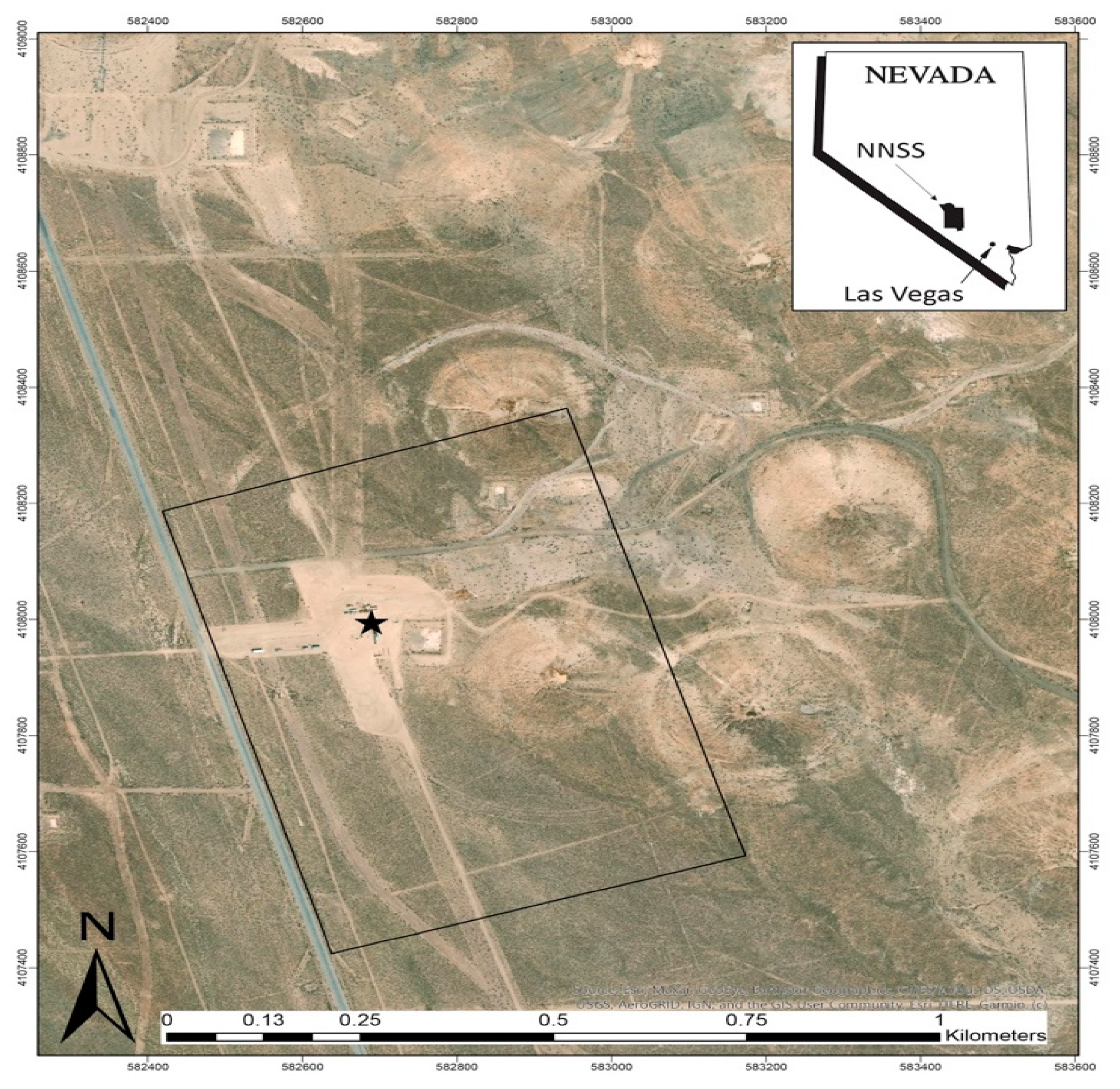
2.1. Setting
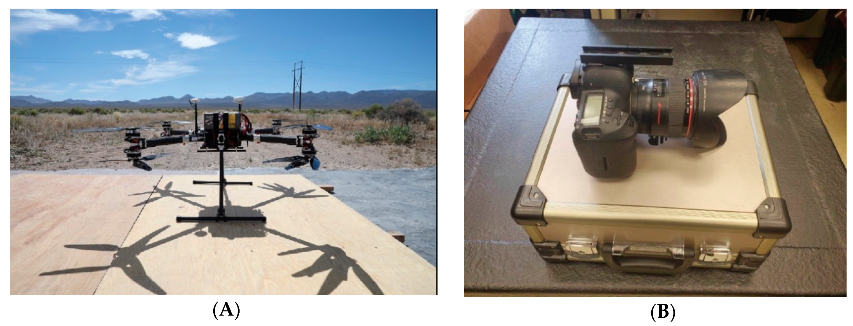
2.2. UAS Equipment
2.2.1. The Airframe
2.2.2. The Camera
2.2.3. SD Card Set-Up
2.3. Survey Equipment
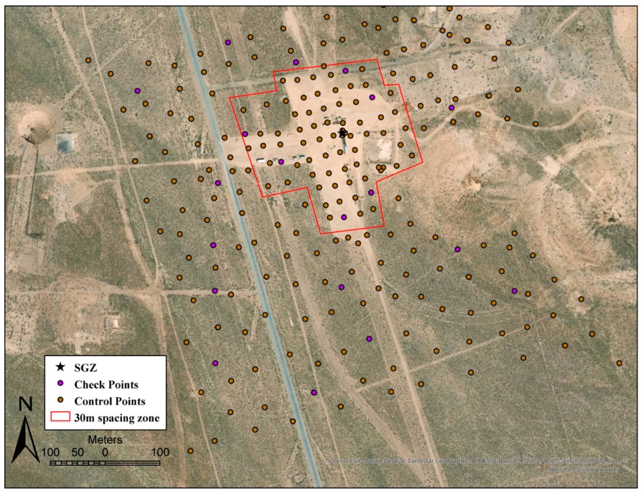
2.3.1. Survey Grid Plan
2.3.2. Survey Procedure
2.4. Flight Operations
2.5. Photo Field Review
2.6. Survey Corrections
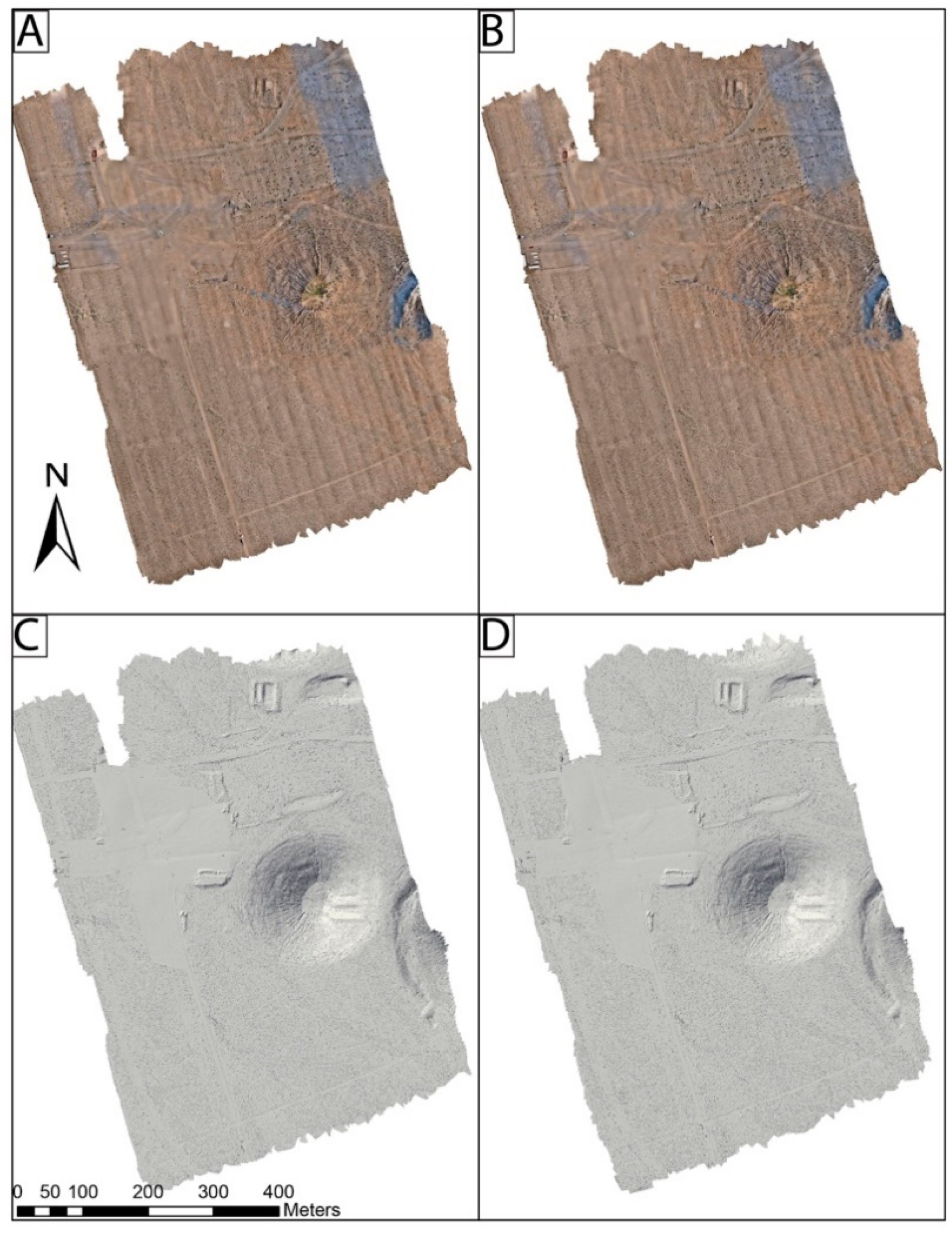
2.7. Creating the Orthoimages and Topographic Models
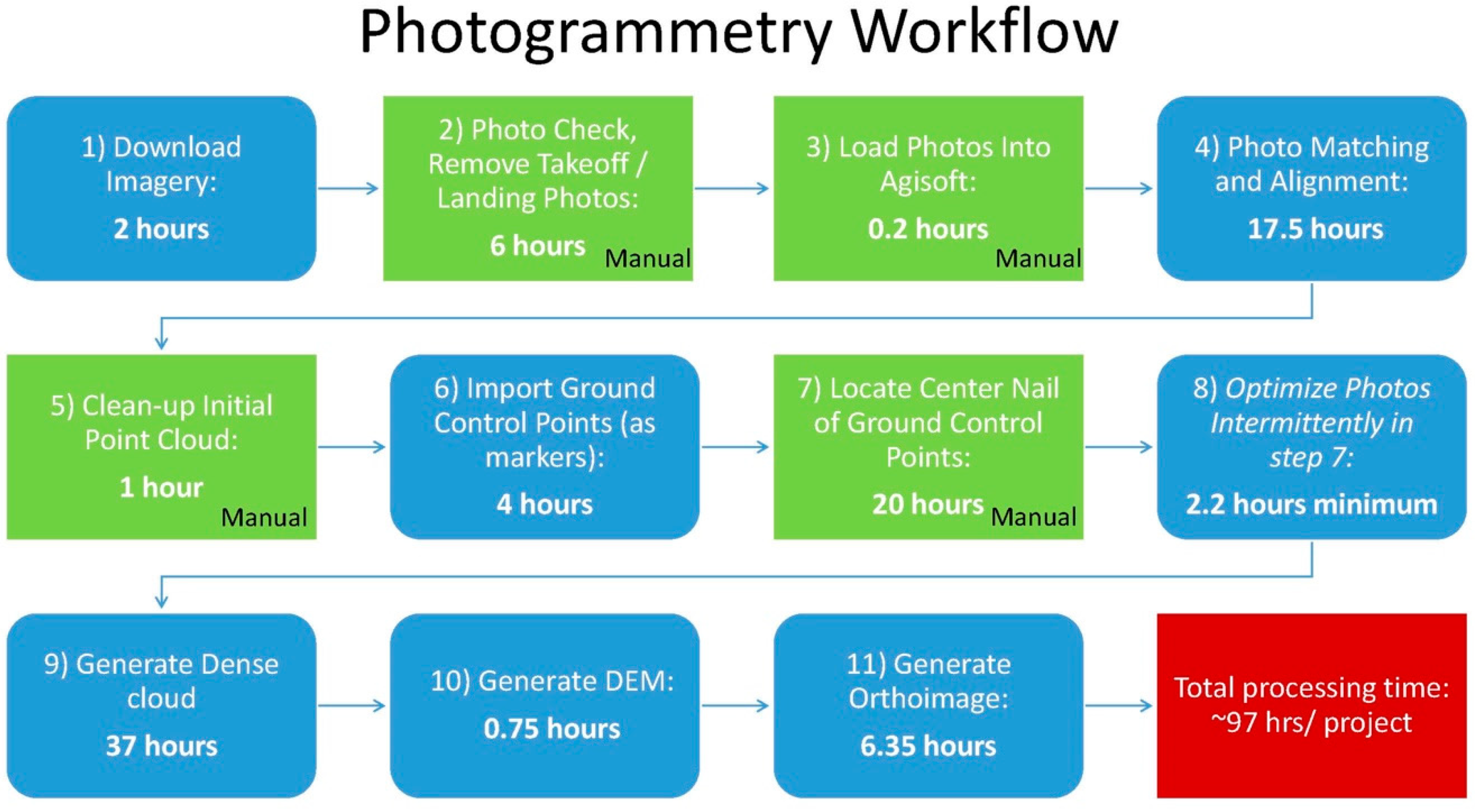
- Download the imagery to external hard drives (usually done in the field, during deployment).
- Check the dataset for completeness, and perform a preliminary filtering, as described in the field methodology above (also completed in the field, or en route back to base camp from the field site).
- Load the imagery into Agisoft Photoscan.
- Use Agisoft Photoscan to stitch photos together by identifying “tie points” in photos that match in adjacent photos. Agisoft then locates each photo’s position relative to those points and creates an initial point cloud from these tie points.
- Following initial photo alignment, edit the tie points using the gradual selection toolset. This removes tie points with large errors, or those which were not tied to a location accurately (which usually arise due to insufficient overlap of photos).
- For each GCP, create a marker within the Agisoft software. Once a marker was identified, it was checked against a map containing all of the GCP locations, to ensure that no points were missing.
- For each marker, filter all of the photos which contain the marker. From these photos we ensured that the estimated location provided by Agisoft was on the center nail of our GCP. If the marker location in any of the photos was not on the center nail, we moved it to that location. This was completed for all markers. Following this, we attempted an initial assessment of the model to find any locations with large vertical or horizontal errors. This was done by looking at the root mean square error (RMSE) for each marker (automatically calculated by Agisoft). RMSE in Agisoft is a measure of the distance between a marker’s surveyed location and the model’s estimated location for that point. Problem areas, defined by large RMSEs, were examined in the sparse cloud, and nearby markers were examined to make sure there were no mis-located center nails. If the large RMSE values persisted, we would readjust the model by: (1) realigning the photos involved in placing the marker, (2) deleting low quality photos, and (3) ensuring the sparse cloud had no anomalous points (above or below the model surface) and deleting them if there were. After the sparse cloud was clean through the initial cleanup, and markers were located, the points were re-projected using the camera calibration tool to attempt to correct any additional distortion caused by the photos themselves. We chose to run the tool with the default settings to avoid over-biasing our photos to match the ground surface. Around 20 markers were selected as check points to help assess the accuracy of the model. These markers used as check points were deselected from use in the model building, and the camera realignment tool was run another time without these markers, affecting the alignment. This effectively provides a second RMSE calculation on the model from points not directly affecting model creation.
- The dense point cloud should be built from the sparse cloud using high settings, and mild depth filtering. This step generally took between 18–28 h, depending on the number of photos, but required little human input and large blocks of dedicated computational processing time.
- Using Agisoft, create the DEM directly from the dense cloud, with the cell size set to 2 cm. We found 2 cm produces a product with high enough resolution to detect small changes, while producing a manageable file size.
- Build the orthoimages from the DEM using a cell size set to 1.5 cm to reduce the final file sizes. For the pre-DAG-2 experiments, we created DEMs and orthoimages at the maximum possible output (cell size of 0.0012 m). This resulted in 1 TB file sizes, which was computationally unwieldy for the full collection area.
2.8. DEMs and Subtraction
3. Results
3.1. Survey Data
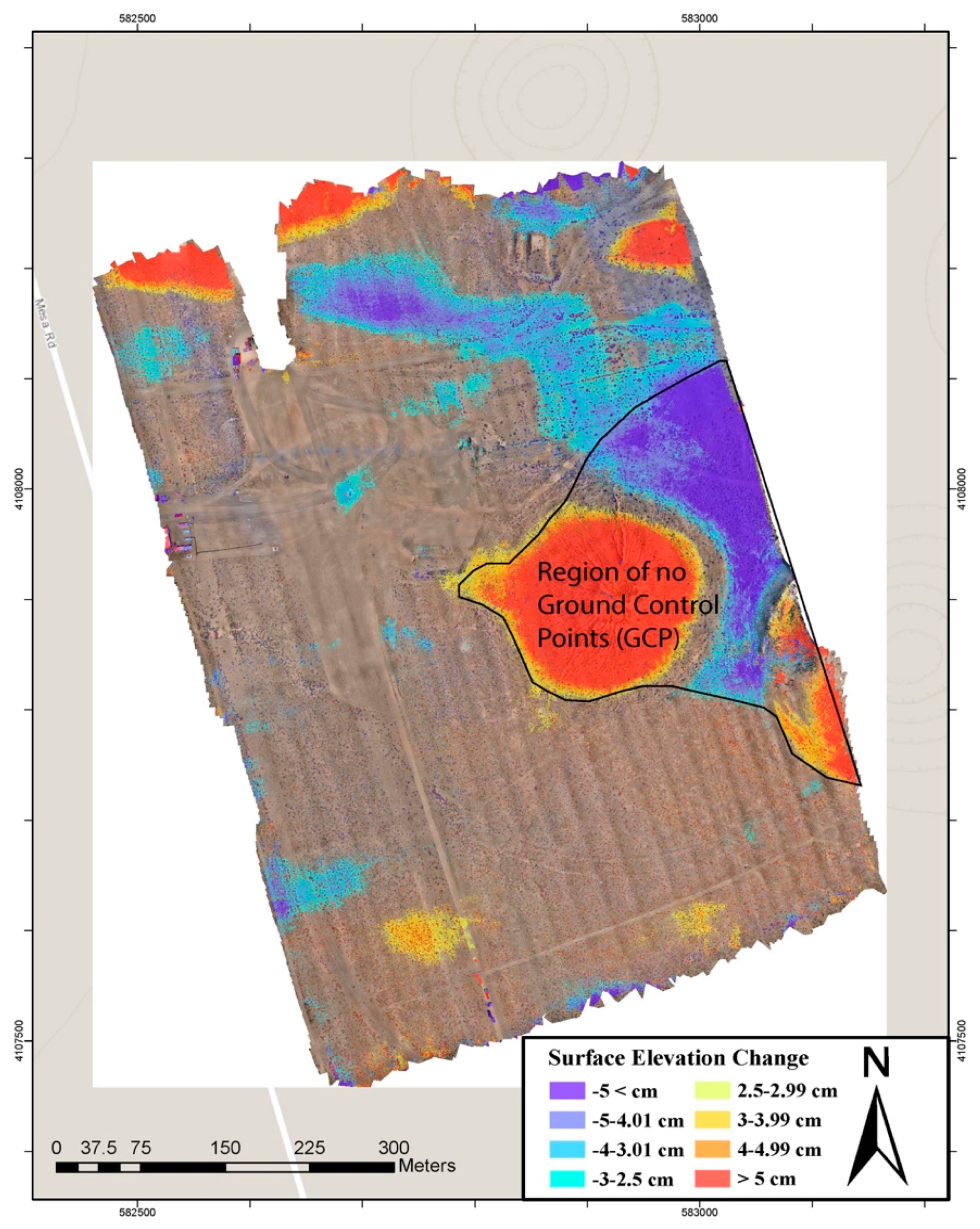
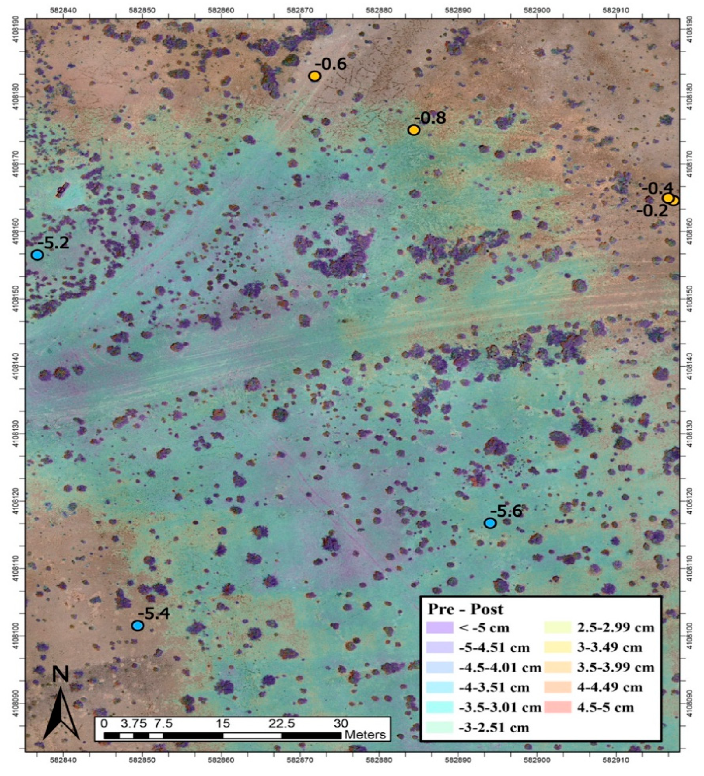
3.2. Topographic Change
3.3. Agisoft Reported RMSE
4. Discussion
4.1. Data Validation
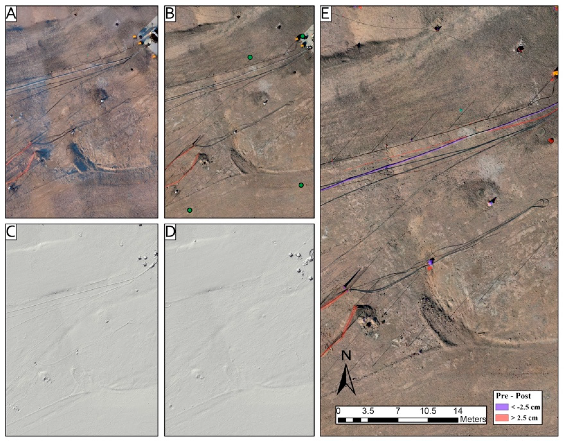
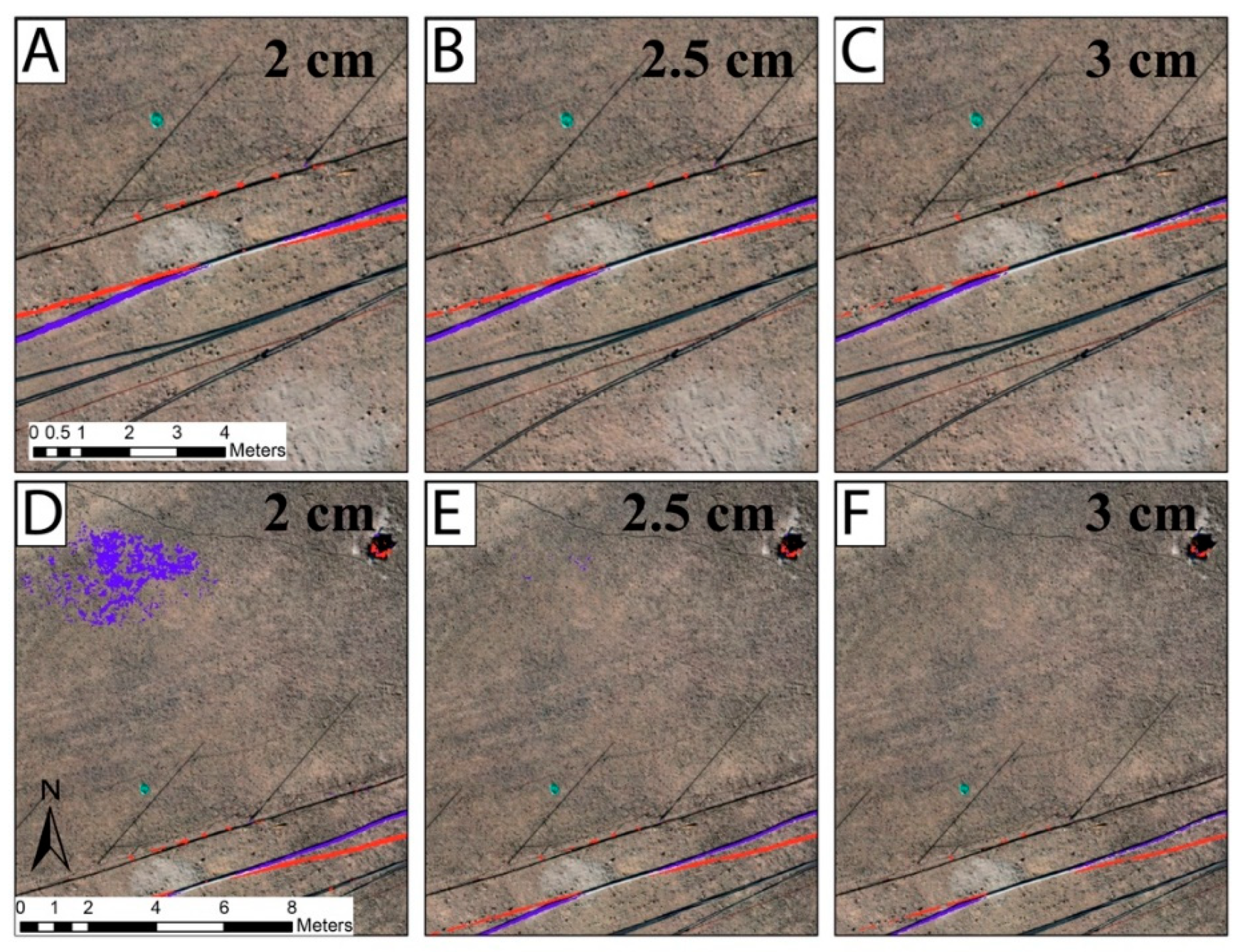
4.2. Discrete Change
4.3. Broad-Scale Change
4.4. Artifacts
5. Conclusions
Author Contributions
Funding
Data Availability Statement
Acknowledgments
Conflicts of Interest
References
- Glenn, N.F.; Streutker, D.R.; Chadwick, D.J.; Thackray, G.D.; Dorsch, S.J. Analysis of LiDAR-derived topographic information for characterizing and differentiating landslide morphology and activity. Geomorphology 2006, 73, 131–148. [Google Scholar] [CrossRef]
- Drǎgut, L.; Eisank, C.; Strasser, T. Local variance for multi-scale analysis in geomorphometry. Geomorphology 2011, 130, 162–172. [Google Scholar] [CrossRef] [Green Version]
- Bemis, S.P.; Micklethwaite, S.; Turner, D.; James, M.R.; Akciz, S.; Thiele, S.T.; Bangash, H.A. Ground-based and UAV-Based photogrammetry: A multi-scale, high-resolution mapping tool for structural geology and paleoseismology. J. Struct. Geol. 2014, 69, 163–178. [Google Scholar] [CrossRef]
- Davies, D.R.; Valentine, A.P.; Kramer, S.C.; Rawlinson, N.; Hoggard, M.J.; Eakin, C.M.; Wilson, C.R. Earth’s multi-scale topographic response to global mantle flow. Nat. Geosci. 2019, 12, 845–850. [Google Scholar] [CrossRef]
- Lindsay, J.B.; Newman, D.R.; Francioni, A. Scale-optimized surface roughness for topographic analysis. Geoscience 2019, 9, 322. [Google Scholar] [CrossRef] [Green Version]
- Liao, J.; Shen, S. Detection of land surface change due to the Wenchuan earthquake using multitemporal advanced land observation satellite-phased array type L-band synthetic aperture radar data. J. Appl. Remote Sens. 2009. [Google Scholar] [CrossRef]
- Kaya, G.T.; Musaoǧlu, N.; Ersoy, O.K. Damage assessment of 2010 Haiti earthquake with post-earthquake satellite image by support vector selection and adaptation. Photogramm. Eng. Remote Sens. 2011, 77, 1025–1035. [Google Scholar] [CrossRef]
- Ishitsuka, K.; Tsuji, T.; Matsuoka, T. Detection and mapping of soil liquefaction in the 2011 Tohoku earthquake using SAR interferometry. Earth Planets Sp. 2013, 64, 1267–1276. [Google Scholar] [CrossRef] [Green Version]
- Menderes, A.; Erener, A.; Sarp, G. Automatic Detection of Damaged Buildings after Earthquake Hazard by Using Remote Sensing and Information Technologies. Procedia Earth Planet. Sci. 2015, 15, 257–262. [Google Scholar] [CrossRef] [Green Version]
- Galloway, D.L.; Hudnut, K.W.; Ingebritsen, S.E.; Phillips, S.P.; Peltzer, G.; Rogez, F.; Rosen, P.A. Detection of aquifer system compaction and land subsidence using interferometric synthetic aperture radar, Antelope Valley, Mojave Desert, California. Water Resour. Res. 1998, 34, 2573–2585. [Google Scholar] [CrossRef]
- Chai, J.C.; Shen, S.-L.; Zhu, H.; Zhang, X. Land subsidence due to groundwater drawdown in Shanghai. Geotechnique 2004, 54, 143–147. [Google Scholar] [CrossRef]
- Higgins, S.; Overeem, I.; Tanaka, A.; Syvitski, J.P.M. Land subsidence at aquaculture facilities in the Yellow River delta, China. Geophys. Res. Lett. 2013, 40, 3898–3902. [Google Scholar] [CrossRef]
- Erban, L.E.; Gorelick, S.M.; Zebker, H.A. Groundwater extraction, land subsidence, and sea-level rise in the Mekong Delta, Vietnam. Environ. Res. Lett. 2014, 9, 084010. [Google Scholar] [CrossRef]
- Phang, M.K.; Simpson, T.A.; Brown, R.C. Investigation of Blast-Induced Underground Vibrations from Surface Mining; Department of Interior Office of Surface Mining Report, U.S.; 1983. [Google Scholar]
- Chowdhury, A.H.; Wilt, T.E. Characterizing Explosive Effects on Underground Structures; U.S. Nuclear Regulatory Commission report NUREG/CR-7201, U.S.; 2015. [Google Scholar]
- Westoby, M.J.; Brasington, J.; Glasser, N.F.; Hambrey, M.J.; Reynolds, J.M. “Structure-from-Motion” photogrammetry: A low-cost, effective tool for geoscience applications. Geomorphology 2012, 179, 300–314. [Google Scholar] [CrossRef] [Green Version]
- Howell, R.G.; Jensen, R.R.; Petersen, S.L.; Larsen, R.T. Measuring Height Characteristics of Sagebrush (Artemisia sp.) Using Imagery Derived from Small Unmanned Aerial Systems (sUAS). Drones 2020, 4, 6. [Google Scholar] [CrossRef] [Green Version]
- Kameyama, S.; Sugiura, K. Estimating Tree Height and Volume Using Unmanned Aerial Vehicle Photography and SfM Technology, with Verification of Result Accuracy. Drones 2020, 4, 19. [Google Scholar] [CrossRef]
- Javernick, L.; Brasington, J.; Caruso, B. Modeling the topography of shallow braided rivers using Structure-from-Motion photogrammetry. Geomorphology 2014, 213, 166–182. [Google Scholar] [CrossRef]
- Neugirg, F.; Stark, M.; Kaiser, A.; Vlacilova, M.; Della Seta, M.; Vergari, F.; Schmidt, J.; Becht, M.; Haas, F. Erosion processes in calanchi in the Upper Orcia Valley, Southern Tuscany, Italy based on multitemporal high-resolution terrestrial LiDAR and UAV surveys. Geomorphology 2016, 269, 8–22. [Google Scholar] [CrossRef]
- Bash, E.A.; Moorman, B.J.; Menounos, B.; Gunther, A. Evaluation of SfM for surface characterization of a snow-covered glacier through comparison with aerial lidar. J. Unmanned Veh. Syst. 2020, 139, 1–21. [Google Scholar] [CrossRef]
- Cucchiaro, S.; Cavalli, M.; Vericat, D.; Crema, S.; Llena, M.; Beinat, A.; Marchi, L.; Cazorzi, F. Monitoring topographic changes through 4D-structure-from-motion photogrammetry: Application to a debris-flow channel. Environ. Earth Sci. 2018, 77, 1–21. [Google Scholar] [CrossRef]
- Agüera-Vega, F.; Carvajal-Ramírez, F.; Martínez-Carricondo, P. Assessment of photogrammetric mapping accuracy based on variation ground control points number using unmanned aerial vehicle. Meas. J. Int. Meas. Confed. 2017, 98, 221–227. [Google Scholar] [CrossRef]
- Martínez-Carricondo, P.; Agüera-Vega, F.; Carvajal-Ramírez, F.; Mesas-Carrascosa, F.J.; García-Ferrer, A.; Pérez-Porras, F.J. Assessment of UAV-photogrammetric mapping accuracy based on variation of ground control points. Int. J. Appl. Earth Obs. Geoinf. 2018, 72, 1–10. [Google Scholar] [CrossRef]
- Čerňava, J.; Chudý, F.; Tunák, D.; Saloň, Š.; Vyhnáliková, Z. The vertical accuracy of digital terrain models derived from the close-range photogrammetry point cloud using different methods of interpolation and resolutions. Cent. Eur. For. J. 2019, 66, 198–205. [Google Scholar] [CrossRef]
- Tonkin, T.N.; Midgley, N.G.; Graham, D.J.; Labadz, J.C. The potential of small unmanned aircraft systems and structure-from-motion for topographic surveys: A test of emerging integrated approaches at Cwm Idwal, North Wales. Geomorphology 2014, 226, 35–43. [Google Scholar] [CrossRef] [Green Version]
- Villanueva, J.K.S.; Blanco, A.C. Optimization of ground control point (GCP) configuration for unmanned aerial vehicle (UAV) survey using structure from motion (SFM). Int. Arch. Photogramm. Remote Sens. Spat. Inf. Sci. ISPRS Arch. 2019, 42, 167–174. [Google Scholar] [CrossRef] [Green Version]
- Meinen, B.U.; Robinson, D.T. Mapping erosion and deposition in an agricultural landscape: Optimization of UAV image acquisition schemes for SfM-MVS. Remote Sens. Environ. 2020, 239, 111666. [Google Scholar] [CrossRef]
- Melita, C.D.; Guastella, D.C.; Cantelli, L.; Di Marco, G.; Minio, I.; Muscato, G. Low-Altitude Terrain-Following Flight Planning for Multirotors. Drones 2020, 4, 26. [Google Scholar] [CrossRef]
- Tonkin, T.N.; Midgley, N.G. Ground-control networks for image based surface reconstruction: An investigation of optimum survey designs using UAV derived imagery and structure-from-motion photogrammetry. Remote Sens. 2016, 8, 786. [Google Scholar] [CrossRef] [Green Version]
- Nagendran, S.K.; Tung, W.Y.; Mohamad Ismail, M.A. Accuracy assessment on low altitude UAV-borne photogrammetry outputs influenced by ground control point at different altitude. IOP Conf. Ser. Earth Environ. Sci. 2018, 169, 1–9. [Google Scholar] [CrossRef]
- Jóźków, G.; Toth, C. Georeferencing experiments with UAS imagery. ISPRS Ann. Photogramm. Remote Sens. Spat. Inf. Sci. 2014, II–1, 25–29. [Google Scholar] [CrossRef] [Green Version]
- Carbonneau, P.E.; Dietrich, J.T. Cost-effective non-metric photogrammetry from consumer-grade sUAS: Implications for direct georeferencing of structure from motion photogrammetry. Earth Surf. Process. Landforms 2017, 42, 473–486. [Google Scholar] [CrossRef] [Green Version]
- Kalacska, M.; Lucanus, O.; Arroyo-Mora, J.P.; Laliberté, É.; Elmer, K.; Leblanc, G.; Groves, A. Accuracy of 3d landscape reconstruction without ground control points using different uas platforms. Drones 2020, 4, 13. [Google Scholar] [CrossRef] [Green Version]
- Sanz-Ablanedo, E.; Chandler, J.H.; Rodríguez-Pérez, J.R.; Ordóñez, C. Accuracy of Unmanned Aerial Vehicle (UAV) and SfM photogrammetry survey as a function of the number and location of ground control points used. Remote Sens. 2018, 10, 1606. [Google Scholar] [CrossRef] [Green Version]
- James, M.R.; Robson, S.; Smith, M.W. 3-D uncertainty-based topographic change detection with structure-from-motion photogrammetry: Precision maps for ground control and directly georeferenced surveys. Earth Surf. Process. Landforms 2017, 42, 1769–1788. [Google Scholar] [CrossRef]
- Schultz-Fellenz, E.S.; Coppersmith, R.T.; Sussman, A.J.; Swanson, E.M.; Cooley, J.A. Detecting Surface Changes from an Underground Explosion in Granite Using Unmanned Aerial System Photogrammetry. Pure Appl. Geophys. 2017, 175, 3159–3177. [Google Scholar] [CrossRef] [Green Version]
- Schultz-Fellenz, E.S.; Swanson, E.M.; Sussman, A.J.; Coppersmith, R.T.; Kelley, R.E.; Miller, E.D.; Crawford, B.M.; Lavadie-Bulnes, A.F.; Cooley, J.R.; Vigil, S.R.; et al. High-resolution surface topographic change analyses to characterize a series of underground explosions. Remote Sens. Environ. 2020, 246. [Google Scholar] [CrossRef]
- Wilmarth, V.R.; McKeown, F.A. Structural Effects of Rainier, Logan, and Blanca Underground Nuclear Explosions, Nevada Test Site, Nye County, Nevada; U.S. Geological Survey Prof. Paper. 400–B, U.S.; 1960. [Google Scholar]
- Barosh, P.J. Relationships of Explosion-Produced Fracture Patterns to Geologic Structure in Yucca Flat, Nevada Test Site; Nevada Test Site. Geol. Soc. Am. Memoir 110, U.S.; 1968. [Google Scholar]
- Dickey, D. Fault Displacement as a Result of Underground Nuclear Explosions; Nevada Test Site. Geol. Soc. Am. Memoir 110, U.S.; 1968. [Google Scholar]
- Morris, R. Topographic and Isobase Maps of the Cannikin Sink, Amchitka Island, Alaska; U.S. Geological Survey Technical Report USGS-474-175, U.S.; 1973. [Google Scholar]
- App, F. Permanent Displacement of the Ground Surface Resulting from Underground-Nuclear-Test-Induced Ground Shock; Lawrence Livermore National Laboratory Report CONF-850953, U.S.; 1985. [Google Scholar]
- Snelson, C.M.; Abbott, R.E.; Broome, S.T.; Mellors, R.J.; Patton, H.J.; Sussman, A.J.; Townsend, M.J.; Walter, W.R. Chemical explosion experiments to improve nuclear test monitoring. EOS Trans. Am. Geophys. Union 2013, 94, 237–239. [Google Scholar] [CrossRef]
- Machado, M. f3—Fight Flash Fraud. Available online: https://fight-flash-fraud.readthedocs.io/en/latest/introduction.html (accessed on 20 May 2018).
- Chao, J.; Chen, H.; Eckehard, S. On the design of a novel jpeg quantization table for improved feature detection performance. IEEE Int. Conf. Image Process. 2013, 1675–1679. [Google Scholar] [CrossRef]
- Akçay, Ö.; Erenoğlu, R.C.; Avşar, E.Ö. the Effect of Jpeg Compression in Close Range Photogrammetry. Int. J. Eng. Geosci. 2017, 2, 35–40. [Google Scholar] [CrossRef] [Green Version]
- Alfio, V.S.; Costantino, D.; Pepe, M. Influence of image tiff format and jpeg compression level in the accuracy of the 3d model and quality of the orthophoto in uav photogrammetry. J. Imaging 2020, 6, 30. [Google Scholar] [CrossRef]
- James, M.R.; Robson, S. Mitigating systematic error in topographic models derived from UAV and ground-based image networks. Earth Surf. Process. Landf. 2014, 39, 1413–1420. [Google Scholar] [CrossRef] [Green Version]
- Nesbit, P.R.; Hugenholtz, C.H. Enhancing UAV-SfM 3D model accuracy in high-relief landscapes by incorporating oblique images. Remote Sens. 2019, 11, 239. [Google Scholar] [CrossRef] [Green Version]


| GCP Name | Δ Easting (cm) | Δ Northing (cm) | Δ Elevation (cm) |
|---|---|---|---|
| 0e + 1 | 1.29 | 0.67 | 0.97 |
| 2a + | 1.63 | 1.41 | 2.11 |
| 2e + | 0.54 | 0.18 | 1.18 |
| 4d + | 1.43 | 1.65 | 0.25 |
| 6d + | 1.66 | 1.81 | 1.29 |
| 7r | 0.20 | 0.32 | 0.60 |
| 11c | 0.29 | 0.03 | 0.53 |
| post g1 | 0.13 | 0.28 | 0.25 |
| post 3i + | 1.46 | 1.94 | 0.98 |
| post 4d + | 1.66 | 1.20 | 0.14 |
| post 3h + | 0.35 | 1.73 | 0.90 |
| Average | 0.97 | 1.02 | 0.84 |
| Name | X-Error (cm) | Y-Error (cm) | Z-Error (cm) | XY-Error (cm) | Total (cm) |
|---|---|---|---|---|---|
| DAG4-Pre Control | 0.887 | 0.938 | 0.551 | 1.291 | 1.403 |
| DAG4-Pre Check | 1.439 | 1.089 | 0.947 | 1.805 | 2.038 |
| DAG4-Post Control | 1.001 | 1.145 | 0.533 | 1.520 | 1.611 |
| DAG4-Post Check | 1.287 | 1.098 | 1.391 | 1.613 | 2.190 |
| DAG4- All Control | 0.944 | 1.041 | 0.542 | 1.406 | 1.507 |
| DAG4- All Check | 1.363 | 1.093 | 1.169 | 1.709 | 2.114 |
Publisher’s Note: MDPI stays neutral with regard to jurisdictional claims in published maps and institutional affiliations. |
© 2021 by the authors. Licensee MDPI, Basel, Switzerland. This article is an open access article distributed under the terms and conditions of the Creative Commons Attribution (CC BY) license (https://creativecommons.org/licenses/by/4.0/).
Share and Cite
Crawford, B.; Swanson, E.; Schultz-Fellenz, E.; Collins, A.; Dann, J.; Lathrop, E.; Milazzo, D. A New Method for High Resolution Surface Change Detection: Data Collection and Validation of Measurements from UAS at the Nevada National Security Site, Nevada, USA. Drones 2021, 5, 25. https://0-doi-org.brum.beds.ac.uk/10.3390/drones5020025
Crawford B, Swanson E, Schultz-Fellenz E, Collins A, Dann J, Lathrop E, Milazzo D. A New Method for High Resolution Surface Change Detection: Data Collection and Validation of Measurements from UAS at the Nevada National Security Site, Nevada, USA. Drones. 2021; 5(2):25. https://0-doi-org.brum.beds.ac.uk/10.3390/drones5020025
Chicago/Turabian StyleCrawford, Brandon, Erika Swanson, Emily Schultz-Fellenz, Adam Collins, Julian Dann, Emma Lathrop, and Damien Milazzo. 2021. "A New Method for High Resolution Surface Change Detection: Data Collection and Validation of Measurements from UAS at the Nevada National Security Site, Nevada, USA" Drones 5, no. 2: 25. https://0-doi-org.brum.beds.ac.uk/10.3390/drones5020025