


Impact of Drone Battery Recharging Policy on Overall Carbon Emissions: The Traveling Salesman Problem with Drone
Department of Industrial Engineering, Bursa Uludağ University, Bursa 16059, Türkiye
Drones 2024, 8(3), 108; https://0-doi-org.brum.beds.ac.uk/10.3390/drones8030108
Submission received: 13 December 2023
/
Revised: 11 March 2024
/
Accepted: 17 March 2024
/
Published: 20 March 2024
(This article belongs to the Special Issue Advances of Drones in Logistics)
Abstract
:This study investigates the traveling salesman problem with drone (TSP-D) from a sustainability perspective. In this problem, a truck and a drone simultaneously serve customers. Due to the limited battery and load capacity, the drone temporarily launches from and returns to the truck after each customer visit. Previous studies indicate the potential of deploying drones to reduce delivery time and carbon emissions. However, they assume that the drone battery is swapped after each flight. In this study, we analyze the carbon emissions of the TSP-D under the recharging policy and provide a comparative analysis with the swapping policy. In the recharging policy, the drone is recharged simultaneously on top of the truck while the truck travels. A simulated annealing algorithm is proposed to solve this problem. The computational results demonstrate that the recharging policy can provide faster delivery and lower emissions than the swapping policy if the recharging is fast enough.
1. Introduction
Recent developments in drone technology have led to the idea of drone usage in last-mile delivery beyond military operations. On the one hand, drones can access difficult terrains and travel faster than classical delivery trucks because the street networks do not constrain their path. In addition, drones have no exposure to congestion. However, they must return to a base because of their limited endurance and load capacity. On the other hand, trucks have a huge load and fuel capacity but might be restricted due to land conditions and congestion. These complementary features of the drone and the truck have given rise to their coordinated use in logistics operations. As a result of these attempts, the traveling salesman problem with drone (TSP-D) has emerged.
In the TSP-D, the truck and the drone concurrently visit customers. The truck is designed to carry the drone on its roof and launch it temporarily. The drone’s load capacity is assumed to be one; thus, it returns to the truck after each delivery. The package of the subsequent customer is loaded, and the drone battery is swapped with a new/fully recharged one. After landing, the drone can depart for another customer visit or travel on top of the truck. The delivery is completed when the last vehicle arrives at the depot, and the objective is to minimize the delivery completion time. This new delivery model has drawn the attention of practitioners. Some e-commerce, parcel delivery, and retail companies, such as Amazon, DHL, UPS, Flirty, and FedEx, have announced their plans to incorporate drones into their operations [1]. In addition to industry practitioners, researchers have also become interested in the problem. Earlier studies mostly analyzed drone integration in parcel delivery [2,3,4]. Further studies incorporated real-life scenarios, such as time windows [5,6], multiple drones [7,8], multiple trucks [9], multiple trucks and drones [10], realistic energy consumption [11,12], and edge launch ability [13,14].
As state-of-the-art studies reveal the potential of drones to reduce delivery time and cost, aiming at widespread drone use, drones must be investigated from a sustainability perspective. They are expected to reduce the carbon footprint through having lower carbon emissions and less energy consumption than classical diesel vans [15]. However, Figliozzi [16] reports that drones tend to be environmentally friendly depending on the density of populated areas, number of customers, and payloads. Goodchild and Toy [17] provide similar conclusions regarding carbon emissions. The impact of employing drones in conjunction with delivery trucks on carbon emissions and cost was investigated by Chiang et al. [18]. They concluded that this delivery concept can reduce the number of trucks, fuel consumption, and carbon emissions.
The studies above assume that the battery is swapped after each flight. Es Yurek and Ozmutlu [19] investigated the TSP-D under a flexible recharging policy. They assumed that the drone was simultaneously recharged while traveling on the truck in tandem. They analyzed the delivery times under two recharging policies: full and partial. In full recharging, the drone cannot launch before the battery is completely recharged. This assumption is relaxed in the partial recharging policy. They also provided an empirical study comparing the swapping and recharging policies under varying recharging rates, swapping times, and battery capacities. This revealed that the recharging policy can reduce the delivery time depending on the speed and customer density. Thus, it is vital to determine whether recharging contributes to reducing carbon emissions while minimizing delivery times. The objective of this study is to answer this question. It makes two main contributions:
- The carbon emission of the TSP-D is quantified by considering the recharging and swapping policies under varying parameters, and a comparative analysis is provided. To our knowledge, this is the first study analyzing the TSP-D under different battery policies from a sustainability perspective.
- A simulated annealing algorithm is proposed to solve large instances of the TSP-D under battery recharging. Since the recharging policy entails updating the battery level as the drone travels on top of the truck, the solution algorithms developed for the swapping policy cannot be used for this problem. Two studies [19,20] propose mathematical formulations to solve this problem. They extend the problem size to 20 and 50 customers by solving the formulations in a heuristic manner. Thus, this study contributes to the literature by providing a solution approach.
The remainder of the study is organized as follows. Section 2 reviews the literature on coordinated delivery. In Section 3, we describe the problem. The solution approach is explained in detail in Section 4. We present the computational results and parametric analysis in Section 5 and then conclude the paper in Section 6.
2. Literature Review
The number of studies on the TSP-D in literature is rapidly growing. The earlier works investigated the synchronization of a truck and a drone. As these studies indicated the efficiency of drone deployment in delivery, further studies focused on incorporating real-world extensions.
2.1. Delivery Performance
Murray and Chu [2] introduced a coordinated delivery approach involving a truck and a drone. In addition to a mathematical model that can solve instances of up to 10 customers, they proposed a heuristic approach constructed on the TSP. They first obtained a truck route and split it into drone tours regarding cost savings. Es Yurek and Ozmutlu [4] developed a two-stage iterative solution approach. In the first stage, they determined the truck route for a given subset of customers and then solved an MILP to assign drone tours optimally in the second stage. Vasquez et al. [21] applied Benders’ decomposition using a similar approach, obtaining the truck route for a subset of customers in the master problem and optimizing drone tours in the subproblem. Agatz et al. [3] allowed the truck to remain stationary and wait for the drone at the launch node. They developed a new formulation based on the enumeration of drone and truck route combinations between each possible launch and rendezvous node. Their results were improved through dynamic programming and applied to larger instances [22]. Their study shows that restricting the truck’s travel during the drone flight can significantly reduce the solution time. Dell’Amico et al. [23] presented a branch-and-bound algorithm that can solve instances involving up to 15 customers. In another study [24], they developed three formulations enhanced by diminishing the number of “big-M” constraints. Performance was quantified by solving 20-customer instances. The TSP-D assumes that the drone hovers while waiting for the truck at the rendezvous node. This was relaxed by Dell’Amico et al. [25], and the drone could land at the customer node to save battery charge. Boccia et al. [26] solved several instances with 20 nodes by combining a branch-and-cut algorithm with a column generation procedure. They proposed dealing with synchronization constraints through column generation. Schermer et al. [27] also proposed a branch-and-cut algorithm to solve 20-customer instances within a one-hour runtime limit. El-Adle et al. [28] developed an MILP formulation and enhanced its tractability with valid inequalities, preprocessing, and bound-tightening strategies.
Some researchers mainly focus on heuristic approaches. de Freitas and Penna [29] proposed a hybrid heuristic algorithm. Inspired by Murray and Chu [2], they obtained a TSP solution and then produced an initial TSP-D solution by assigning some truck nodes to the drone and considering cost savings. General Variable Neighborhood Search (GVNS) was applied to improve the initial solution. Another hybrid heuristic algorithm was presented by Ha et al. [30]. Initial solutions were generated through a genetic algorithm. Then, a split procedure was applied to obtain truck and drone chromosomes. The quality of the solutions was improved through a local search. They incorporated a repairing mechanism into the hybrid algorithm to repair infeasible chromosomes. Similarly, Kundu et al. [31] developed a two-stage heuristic. They first obtained a TSP tour and split it using the shortest path problem, which is the novelty of the solution approach. The solution was improved by a local search. El-Adle et al. [32] proposed a variable neighborhood search in which intensification was achieved in two stages. Gunay-Sezer et al. [33] improved some of the best-known solutions by presenting a hybrid heuristic algorithm composed of genetic and ant colony algorithms.
Liu et al. [34] investigated the problem with stochastic travel times. This was modeled as a Markov decision problem and solved using a reinforcement learning algorithm. They reported significant savings in the delivery time by dynamic decision making based on traffic conditions.
The above studies assume that the truck can only launch and pick up the drone at customer nodes. Marinelli et al. [13] relaxed this assumption for battery efficiency by allowing launch and pickups along edges. After obtaining a TSP-D solution through a greedy algorithm without relaxation, they improved the solution by intersecting a spanning area of the drone node with the related arcs on the truck route. The experimental study demonstrated that relaxation is helpful when the vehicles travel at the same speed. Masone et al. [14] assumed the drone can carry multiple packages simultaneously. The problem was solved with edge launches using edge discretization.
Some researchers have studied the multi-truck and multi-drone version of the problem. Wang et al. [35] provided a worst-case analysis to reveal the maximum savings obtained in the last-mile delivery by a fleet of trucks equipped with several drones on top. They also provided some bounds demonstrating how the drone speed and the number of drones per truck affect the maximum saving. The same authors extended the previous study considering cost issues and limited battery life [36].
Beyond the theoretical perspective of the early research in the literature, Murray and Raj [7] analyzed the TSP-D, operating a truck and multiple drones with varying battery limits, and proposed a three-stage heuristic approach. The multi-drone case leads to the replenishment order of the arriving (departing) drones at the same rendezvous (launch) node. It is considered a scheduling problem by Dell’Amico et al. [8], who proposed several formulations. Thomas et al. [37] extended this problem by relaxing the assumption that the truck can only launch and pick up the drones at customer nodes. Moshref-Javadi et al. [38] described three delivery models based on the level of synchronization between a truck and several drones. They reported that the maximum saving is obtained with the highest level of synchronization. The congested and clustered instances provided higher saving rates compared to uniforms. Tiniç et al. [39] proposed flow-based and two cut-based models to solve a truck and multi-drone delivery problem with cost minimization. They enhanced the formulation with valid inequalities. Kitjacharoenchai et al. [10] simplified the multiple truck–drone delivery problem based on two assumptions. First, the drones can return to the depot or visit a recharging station when needed. Second, the truck can launch or pick up only one drone at any customer node. The authors provided a mathematical model and a heuristic algorithm based on two phases. Tamke and Buscher [40] developed an MILP formulation and introduced problem-specific valid inequalities to strengthen linear relaxation. They solved 20-node instances, assuming unlimited drone ranges and 30-node instances with range-limited drones. Their study reveals that coordinated delivery can reduce the fleet size so that the delivery speed and the operator’s workload do not deteriorate.
Di Puglia Pugliese and Guerriero [41] extended the problem by incorporating time windows into the truck–drone delivery system. Coindreau et al. [6] assumed drone-eligible customers and time windows. The heuristic results obtained by applying an adaptive large neighborhood search with 100 parcel instances report a decrease of up to 34% in delivery costs. Yin et al. [42] proposed an enhanced branch-and-price-and-cut algorithm for the multiple trucks and multiple drone delivery problem with time windows.
A number of recent studies have investigated heuristic approaches for the multi-truck case. Lei et al. [43] proposed a dynamical artificial bee colony algorithm to minimize operational costs when multiple trucks are equipped with one drone. Kuo et al. [44] formulated an MIP model and proposed a variable neighborhood search heuristic for time window extension. The truck can pick up or launch the drone without parking [45]. This assumption entails synchronization on arcs. A nonlinear programming formulation and an adaptive large neighborhood search heuristic were proposed to solve the problem.
Beyond these extensions, some studies have investigated multi-visit drone flight. Luo et al. [46] studied the TSP-D and allowed for multiple drone visits per flight. The drone performed only delivery services. Energy consumption depends on the drone’s payload, self-weight, and flight time. This study proposed a multi-start tabu search algorithm, revealing that multi-visit drone flight can reduce delivery costs. Liu and Liu [47] solved a similar problem and developed a hybrid heuristic approach. This approach involved first constructing a feasible solution quickly and then improving it through simulated annealing and tabu search algorithms. They reported that, in a 30-customer network, the drone performs 12 deliveries in the single-visit case, whereas it delivers 20 parcels in the multi-visit case. Huang et al. [48] minimized the delivery cost for a similar problem by applying an ant colony algorithm. They concluded that the single-visit case performs better with clustered instances rather than random instances and that, for the multi-visit case, the opposite is true. Meng et al. [49] allowed drones to provide a pickup service in addition to delivery on each flight.
In most of the studies outlined above, the flight time constrained the drone’s travel. However, other parameters, such as payload and energy consumption, can affect drone flight. Campuzano et al. [50] considered the interdependencies among energy consumption, weather conditions, drone payload, and drone speed. Since the drone range depends on energy consumption, they determined the drone speed and the routes to minimize delivery time. The drone speed was discretized, and three levels were specified in their computational study. Mahmoudi and Eshghi [11] evaluated energy consumption based on payload and flight mode: takeoff, cruise, landing, and hovering. In [12], energy consumption depended on the drone load and was formulated as a nonlinear function. Similarly, Jeong et al. [51], Wu et al. [52], and Murray and Raj [7] considered payload-dependent energy consumption while satisfying the flight range. In [46], energy consumption depended on the drone’s payload, self-weight, and flight time.
Contrary to the above studies, Es Yurek and Ozmutlu [19] were the first to investigate the coordinated delivery concept under the battery recharging assumption. They developed an MIP model to solve the problem under full and partial recharging policies. They conducted an extensive computational study comparing the delivery times obtained by recharging and swapping policies under varying battery lives, recharging rates, short and long swapping times, and customer distributions. The results indicate the potential of the recharging policy to reduce delivery time. Tamke and Buscher [20] recently proposed an MIP model to determine routes and drone speed while minimizing delivery costs under the battery recharging policy. When the drone travels faster, the delivery time is reduced; however, the energy consumption increases, which leads to a trade-off between energy consumption and drone speed. Energy consumption was evaluated based on drone speed and payload. The MIP model was tested as a heuristic using 50-customer data.
2.2. Sustainability Performance
The studies reviewed thus far focus on improving delivery performance through cost or delivery time minimization. However, the sustainability performance of the coordinated delivery concept is as significant as operational efficiency. When sustainability is the subject, studies mostly focus on minimizing carbon emissions or energy consumption. Meng et al. [49] investigated coordinated delivery by a truck and a drone from economic and sustainability perspectives. They analyzed the trade-off between carbon emissions and cost. Truck emission is the weight of carbon emitted by the truck during the delivery process, which is evaluated based on fuel consumption, and drone emission is based on the amount of carbon indirectly emitted during the electricity production process. The total cost includes the energy consumption cost, carbon emission cost, and drivers’ wages. A dual-objective MIP model has been formulated to solve this problem. The model was tested on data with ten demand nodes based on a firm in China. The study reported that coordinated delivery can reduce carbon emissions by 24.90%, the total cost by 22.13%, and the delivery time by 20.65% compared to traditional truck-based delivery. Like the authors of [49], Baldisseri et al. [53] analyzed the same system’s cost and emission. However, they compared its performance with three delivery systems: delivery by diesel vans, delivery by electric vans, and delivery by drones. In all cases, the coordinated delivery approach produced the lowest emissions. They defined different scenarios to evaluate carbon emissions. These scenarios were distinguished based on the drone utilization rate, wind speed, truck acceleration, and electricity production mix. Chiang et al. [18] minimized carbon emissions, which were evaluated as proportional to the distance traveled by the truck and the drone. A genetic algorithm was proposed to solve the problem. Banyai [54] minimized energy consumption and greenhouse gas emissions and reported that integrated delivery can significantly reduce energy consumption and emissions.
Zhang et al. [55] minimized the total energy consumption, delivery cost, and delivery time while determining delivery routes. The drone’s energy consumption was neglected since it was slight compared to the truck’s energy consumption, which was evaluated considering the truckload and distance. None of those studies considered the geographic information of the customer locations. Baek et al. [56] maximized battery utilization through energy-efficient routes. Delivery was performed concurrently by an electric truck and a drone. Since the energy consumption of the truck is sensitive to the altitude and road conditions, drone use could lead to efficient battery use by visiting customers located in energy-consuming terrains. The drone battery is not replaced or recharged and is used until it is depleted. However, the drone must return to the truck after each flight due to its payload capacity of one. A greedy heuristic algorithm was proposed to solve this problem. The computational results based on 30-customer data reported truck battery energy savings of up to 69%. Similarly, Xiao et al. [57] considered steep roads and travel distance, payload, and drone speed in energy consumption. They proposed an adaptive large neighborhood search to minimize total energy consumption.
As the reviewed studies have indicated, coordinated truck–drone delivery system’s economic, sustainability, and delivery performances are investigated assuming battery replacement. Although the potential of battery recharging to reduce delivery time has been shown, there is a gap in assessing the sustainability of the recharging policy. This study addresses the TSP-D under the recharging policy, considering sustainability aspects.
3. Problem Description
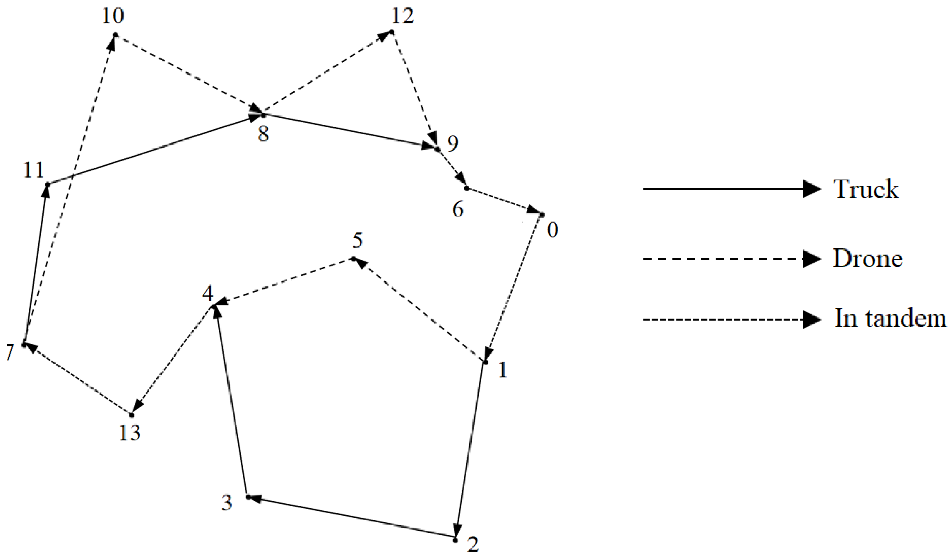
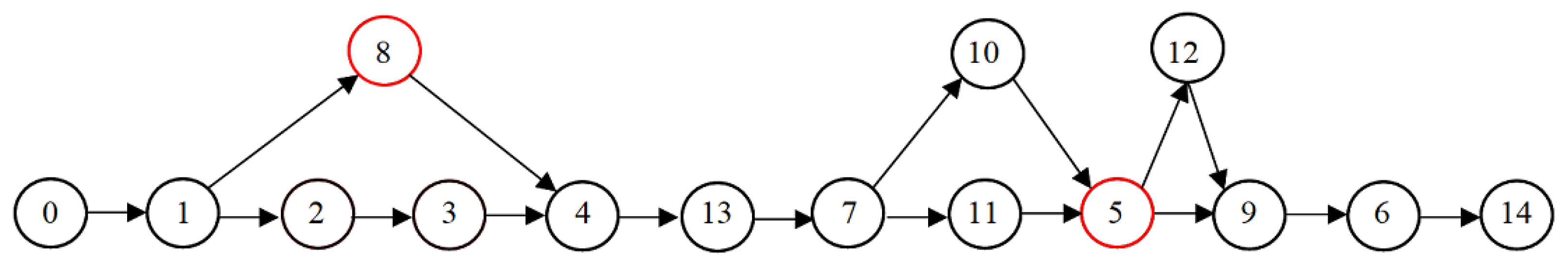
In the recharging policy, the drone battery is recharged through a charge station while the drone travels on the truck’s roof, increasing the charge level. Conversely, it decreases as the drone flies. In Figure 1, the drone travels on top of the truck along the arcs represented by dotted lines. So, the battery is recharged while traveling from Node 0 to Node 1, Node 4 to Node 7, and Node 9 to Node 0. For the remainder of the delivery, the drone performs individual customer visits. Each flight is defined as a drone tour and illustrated by dashed lines. For example, the flight from Node 1 to Node 5 and then to Node 4 is a drone tour. Each drone tour has three nodes: launch, drone, and rendezvous. A flight begins (ends) at the launch (rendezvous) node, whereas any node performing as both is called a mixed node. For example, Node 8 is mixed. The truck keeps traveling and delivering during the drone flight. Its journey between each launch and rendezvous node is defined as a truck-only tour and depicted by the solid lines in the figure. For clarity, we call any combination of a truck-only tour and a drone flight a tour. For example, the tour between Nodes 1 and 4 includes a drone flight and a truck-only tour. If the drone arrives at the rendezvous node before the truck, it waits for the truck to land, and vice versa. So, the tour cost is the cost of the vehicle that arrives last at the rendezvous node.
We make the following assumptions regarding the TSP-D and the implementation of the recharging policy:
- The drone must land on the truck before the battery life expires. While waiting, it hovers and consumes energy.
- The launch and rendezvous can be conducted only at the customer nodes.
- The service time at the customer node is neglected. Thus, only the in-tandem travel time is considered for recharging.
- Recharging can be terminated before the charge level increases to the maximum level.
4. Materials and Method
The TSP-D under the recharging policy is more difficult to solve than the TSP-D under the swapping policy because it entails keeping track of the battery level to ensure feasible flights. The previously mentioned studies indicated that it is impractical to solve realistically sized problems exactly through mathematical formulations. Thus, this study focuses on developing a heuristic algorithm rather than a mathematical model and proposes a simulated annealing algorithm to analyze the TSP-D under the recharging policy from a sustainability perspective. The simulated annealing algorithm is a metaheuristic approach simulating the cooling process in metallurgy [58]. It begins with an initial solution, and then a search process for seeking new solutions is implemented. A new solution is always accepted unless the best objective value deteriorates. A worse solution is accepted with a decreasing probability as the algorithm iterates. The algorithm is terminated when a predefined stopping criterion is met. The implementation of the proposed algorithm is illustrated below.
4.1. Solution Representation
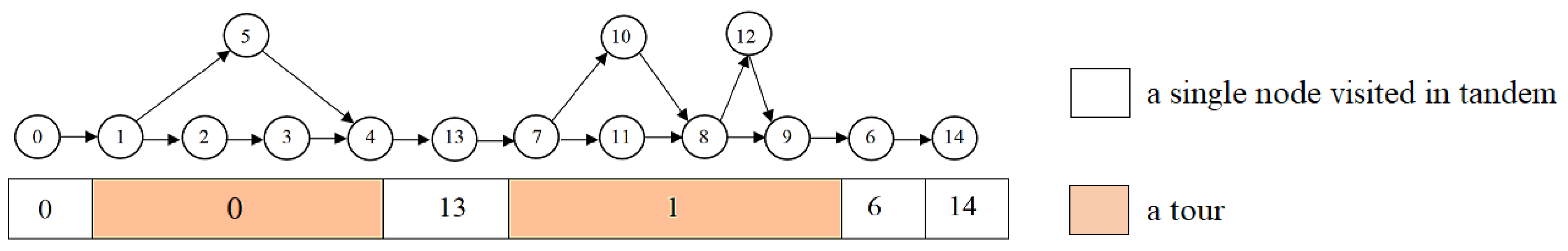
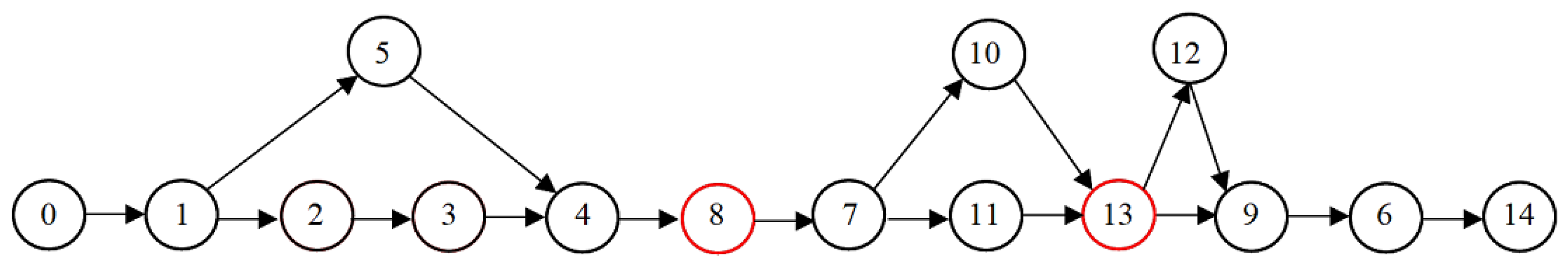
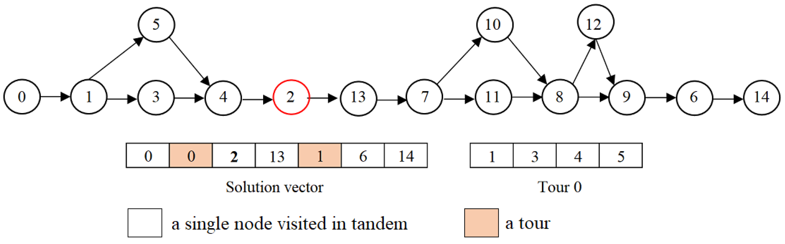
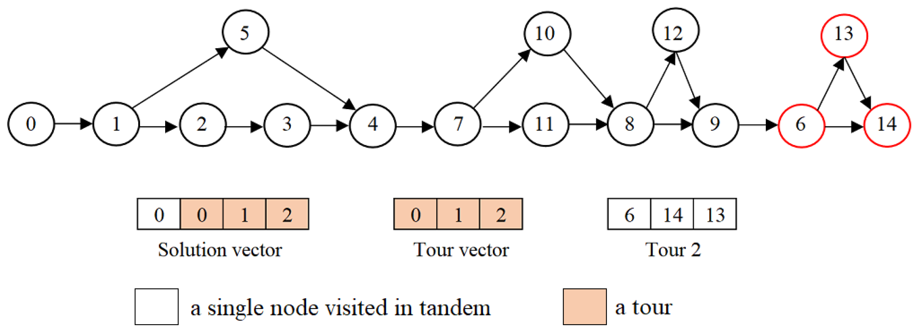
The recharging policy entails keeping track of the charge level throughout the delivery because the charge level moves up and down depending on recharge and discharge. The search process for new solutions can easily lead to infeasibility, which entails checking whether the charge level is sufficient for each subsequent flight. Thus, we propose a solution representation that distinguishes recharge and discharge. A solution is represented by a vector where each element is an object of type operation. An operation object is either a customer visited in tandem or a tour. The delivery route in Figure 1 is encoded in Figure 2. The uncolored elements represent a single node visited in tandem, whereas the colored ones are tours. For each element in the solution vector, we keep some information. First, we must keep the charge level each time a visit has been performed. If it is a single node, the operation is in tandem, implying that the drone’s battery is recharged. For example, the truck leaves Node 4 carrying the drone on top and visits Node 13. During this journey, the battery is recharged. Otherwise, it is a tour. When the drone launches and performs a flight, it consumes energy, and a decrease is indispensable. Therefore, we need to keep the charge level distinct at the beginning and end of each operation. We also need to know the operation type to increase or decrease the charge level.
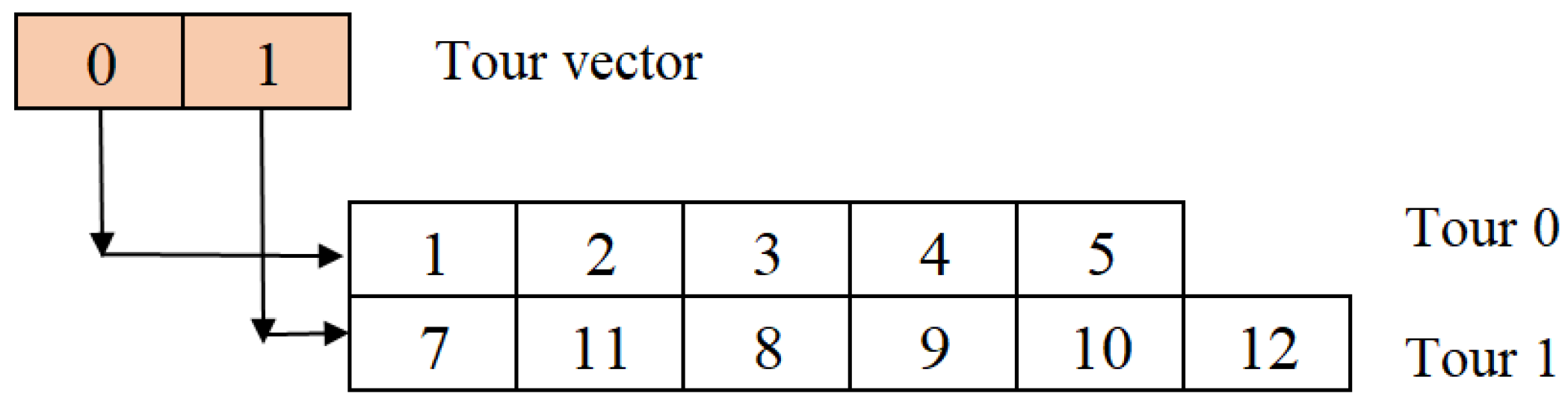
For convenience, a tour is represented by a single element in the solution vector. However, it is a part of the overall delivery route and includes several nodes. So, we keep the details in another vector. Each element of this secondary vector is a tour object, colored in Figure 2. It retains a vector and extra information. The tour vector is depicted in Figure 3, which demonstrates the tours below the tour vector. The encoding procedure places the drone node at the end. Thus, Tour 0 is decoded so that the drone launches at Node 1, serves Customer 5, and returns to the truck at Node 4. Meanwhile, the truck visits Nodes 2 and 3. In the second tour, the drone launches from Node 7, lands on the truck at Node 8 after visiting Node 10, and launches again to visit Node 12. A single element in the solution vector represents these two consecutive tours. The nodes visited by the truck are written first in the vector; then, the drone nodes come. The third element is labeled as a mixed node, implying that Node 8 is both a rendezvous and a launch node. As well as the tour, some extra information is needed, such as the drone cost, truck cost, total cost, mixed node, and number of drone deliveries.
4.2. Construction of Initial Solution
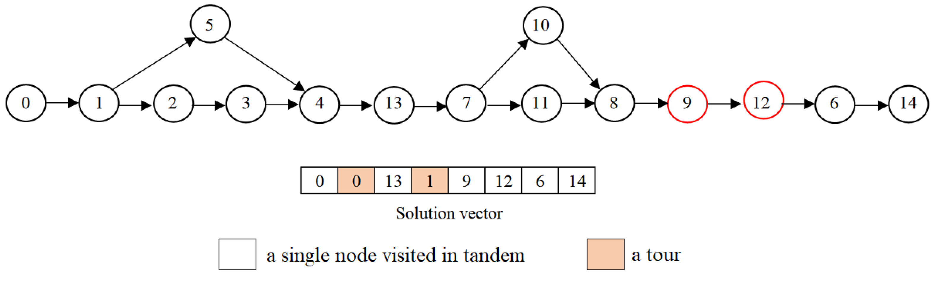
An initial solution is constructed using a greedy algorithm based on the TSP solution. Providing a TSP tour, Algorithm 1 partitions it into drone- and truck-only tours. The algorithm starts from the beginning of the TSP tour, and the position is considered a temporary launch node. Then, it searches all nodes that are likely drone and rendezvous nodes. The nodes providing maximum savings are permanently assigned as the tour’s launch, drone, and rendezvous nodes if a saving is obtained. The drone node is removed from the TSP tour. The algorithm searches for other tours beginning from the last rendezvous node. If a saving is not obtained, the algorithm moves to the next position in the TSP tour and keeps searching for potential tours. For example, we are given a TSP tour 0-1-2-5-3-4-13-7-11-8-12-9-6-14. Node 0 is labeled the temporary launch node, and Node 2 is the temporary rendezvous node. Then, the algorithm calculates the saving when the temporary drone node is Node 1 if it returns feasible truck-only and drone tours smaller than the battery life. Suppose it is infeasible. Then, we consider Node 5 as the temporary rendezvous node. The savings are calculated pretending each node between Node 0 and Node 5 is a temporary drone node. The one with the maximum saving becomes the permanent drone node, and Nodes 0 and 5 become permanent launch and rendezvous nodes, respectively; subsequently, the algorithm searches for new tours starting from Node 5. If the partition does not provide savings or a feasible tour, Nodes 1 and 5 are labeled the new temporary launch and rendezvous nodes, and savings are investigated. The algorithm terminates when the search on the TSP tour is completed.
| Algorithm 1. Pseudocode for constructing the initial solution. |
| Solve TSP and obtain TSP tour with N + 2 elements |
| for all i = 0 to N − 1 do |
| max_saving = 0 |
| sign = 0 |
| for all k = i + 1 to N + 1 do |
| for all j = i + 1 to k − 1 do |
| if j is Drone-eligible then |
| Calculate truck_cost |
| Calculate drone_cost |
| Calculate saving |
| if saving > max_saving and truck_cost < endurance and drone_cost < endurance then |
| l = i |
| d = j |
| r = k |
| sign = 1 |
| end if |
| end if |
| end for |
| end for |
| if sign = 1 then |
| Construct tour |
| i = p |
| end if |
| end for |
4.3. Search Method
A neighbor solution is obtained by applying a local search on the current solution. To do this, we propose several moves in this section. Since our solution vector includes two types of elements, the proposed search method considers this differentiation. The moves are implemented if and only if the feasibility is satisfied.
4.3.1. Swap_in()
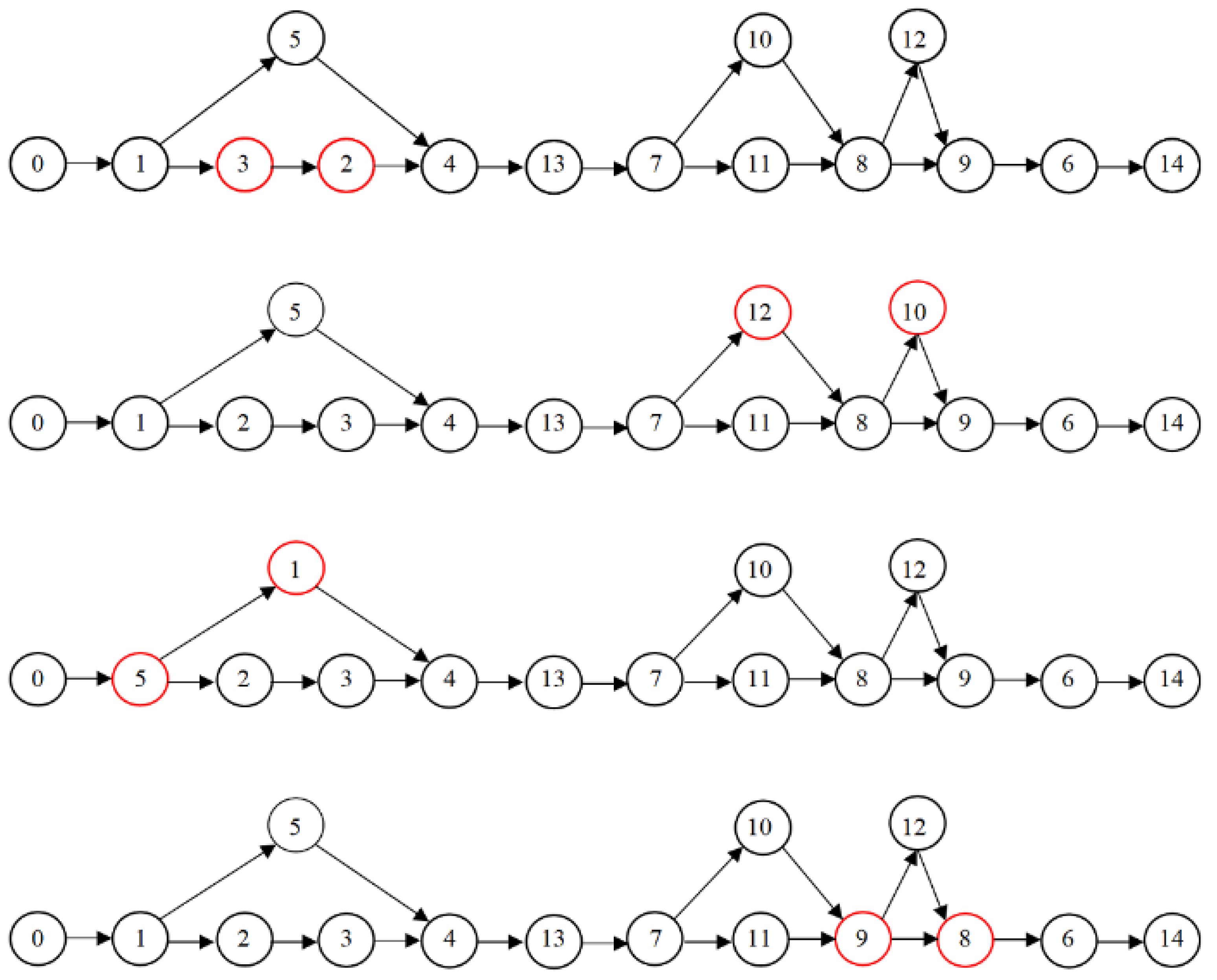
This move intensifies any tour element selected randomly in the solution vector. Each tour includes at least three nodes, and two randomly selected ones are swapped. This move can change the drone and/or truck cost, triggering a chain of actions. A swap can change the total tour cost since a tour’s total cost equals the maximum of the truck and drone costs. If it changes, the battery level changes. A change in the battery level entails the feasibility checks of all subsequent tours and the tour where the swap is performed.
Figure 4 illustrates the swap of different node types on the solution vector depicted in Figure 2. In the first one, two truck-only nodes are swapped. In this case, the truck cost is updated. Suppose the truck cost is smaller than the drone cost and remains the same after the swap; neither the total tour cost nor the solution cost changes. Otherwise, we need to check the total tour cost. In the second solution, two drone nodes in a multi-tour are swapped. Each tour’s drone cost must be compared with the related truck cost. If the total tour cost increases, the charge level decreases. Otherwise, the charge level will increase and not threaten the feasibility. The third solution illustrates the swap of the launch and drone nodes. This move affects the in-tandem travel time before the first tour. Thus, the charge level changes regardless of the new tour cost, leading to the feasibility check of this tour and the subsequent tours. The total tour cost can also change. Similarly, the in-tandem travel time changes when the swap is performed on a rendezvous node.
4.3.2. Swap_cross()
In this move, two tours are selected randomly. Then, two random nodes, each from distinct tours, are swapped. Although the in-tandem nodes remain the same in the solution vector as in swap_in(), this operator can yield a change in the total tour cost and the charge level, which can return infeasibility. For example, Node 5 in the first tour and Node 8 in the second tour are swapped, and the new solution is shown in Figure 5.
4.3.3. Swap_out()
The preceding two moves only focus on exploring tours to improve the solution. They return the same solution vector, but different tours are retained in the tour vector. Unlike the others, this operator swaps a node in a tour and an in-tandem node in the solution. For example, the second tour and the third element of it are selected randomly. It can be swapped with Node 13 or Node 6 because Node 0 and Node 14 denote the source and sink depot, and the route must begin and end at the depot. The solution after the move is provided in Figure 6.
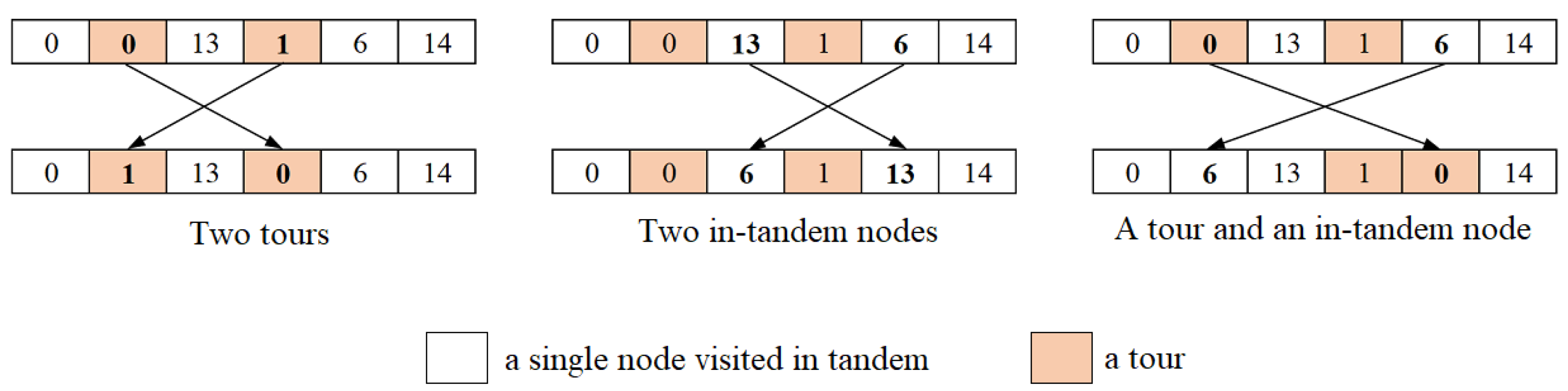
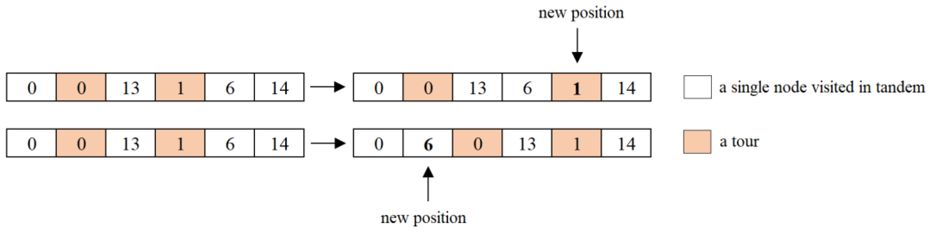
4.3.4. Swap_position()
This move swaps two random elements in the solution vector and can be performed in three ways (Figure 7). First, the swap can be performed between two tour objects. Second, two in-tandem nodes can be swapped. Finally, a tour object can be swapped with an in-tandem node. In none of these scenarios, the nodes in the tour and their sequences change.
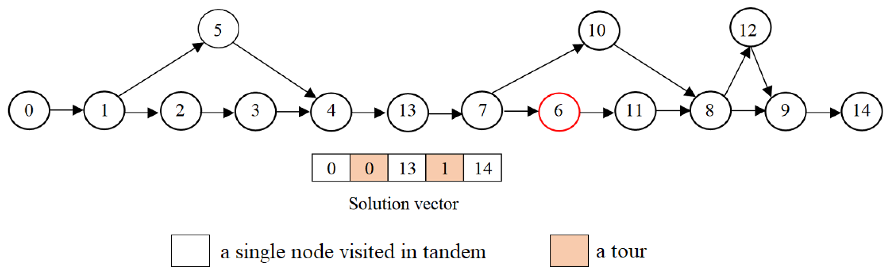
The solution vector after the last swap in Figure 7 is decoded in Figure 8. The second and fifth elements in the solution vector are selected randomly and swapped. Since this move does not amend the tour, the amount of discharge remains the same. However, any change in the sequence of the solution vector can lead to different charge levels. So, the feasibility of both tours must be checked. Although the position of Tour 1 is the same, the change in the second element of the solution vector can cause an insufficient charge level to fly Tour 1. Thus, it needs to be checked as well.
4.3.5. Relocate_in()
We select a random tour with at least one truck-only node. One of the truck-only nodes is selected and relocated. We select a random position in the solution vector to perform this move. If it is an in-tandem node, the selected truck-only node is moved into that position as an in-tandem node. The number of elements in the solution increases by one. For example, Tour 0 and Node 2 are selected. It is relocated into Position 2. This move entails updating Tour 0 and the solution vector. The new solution and the solution vector are demonstrated in Figure 9. Similarly, the charge levels must be updated. However, a feasibility check is unnecessary because there is no increase in the amount of discharge and no decrease in the amount of charge.
If the selected position is a tour, the selected node is inserted in a truck-only position. Suppose Position 3 is randomly selected and represents Tour 1, a multi-tour. Node 2 can be placed anywhere between Nodes 7 and 8 or Nodes 8 and 9. It is randomly relocated, as in Figure 10. In this case, the solution vector remains the same. This move changes only the tours from which the random node is removed and relocated. The total tour costs will likely change, including charge level updates and feasibility checks.
4.3.6. Relocate_out()
This operator moves a random element in the solution vector into a random position. Two examples are illustrated in Figure 11. Tour 1 is relocated in the first vector and Node 6 in the second. Since the charge levels change, the feasibility can be easily unsatisfied.
4.3.7. Insert()
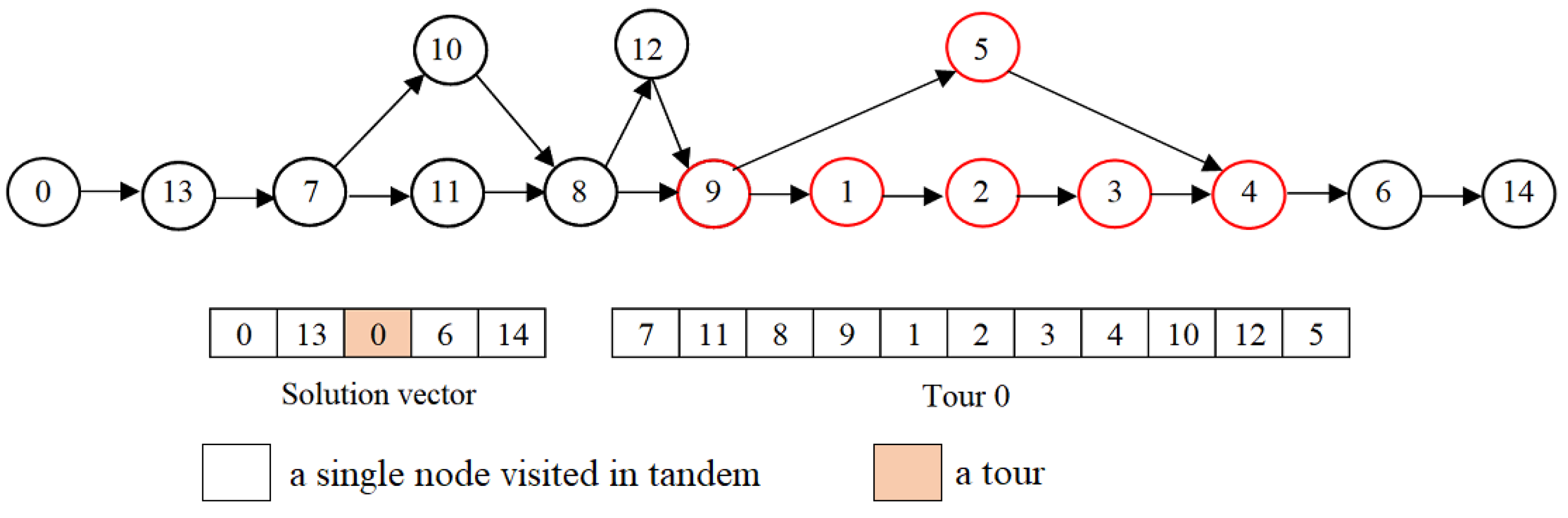
This move removes a random element from the solution vector and inserts it into a random tour. If the selected element is an in-tandem node, it is inserted into a truck-only position. This case is illustrated in Figure 12. If a tour is selected, the insertion is performed so that one of the current tours becomes a multi-tour if it is single, or the number of tours increases if it is already multiple. In any case, the number of elements in the solution vector decreases. This move entails updating the charge levels and checking the feasibility of the subsequent tours.
In Figure 13, Tour 0 is selected and inserted into Tour 1, which is already a multi-tour. This insertion expands it, as it now includes three sub-tours. We note that the launch node of Tour 0 is converted to a truck-only node, and the rendezvous node of Tour 1 is converted to a mixed node. Moreover, Tour 0 is removed from the tour vector, and Tour 1 is labeled Tour 0.
4.3.8. Group()
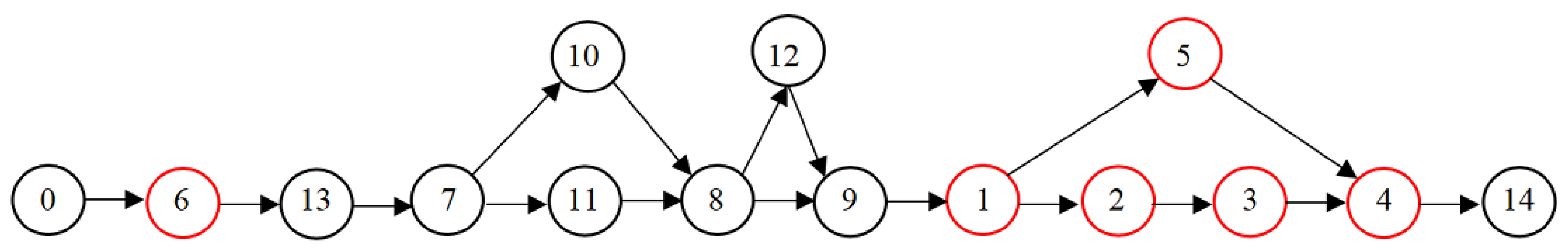
During the search process, the number of in-tandem nodes can increase due to the relocate_in() and destroy() operators. Although this is an opportunity in the recharging policy to allow for sufficient recharging time for the battery, it may also yield a longer delivery time. This move takes three in-tandem nodes and converts them into a tour. First, consecutive nodes are checked for the selection of three in-tandem nodes. Without three successive nodes, or unless a feasible tour is created, they are randomly selected from the solution vector. A certain number of attempts are made to generate a feasible tour. This move reduces the number of in-tandem nodes in the solution vector and increases the number of tours. The position of the new tour in the solution vector is also an important issue. To avoid significant variations in the charge level, we insert it into the end of the solution vector after all the current tours. Implementing this move entails updating both the solution vector and the tour vector. Figure 14 depicts the TSP-D solution after this operator is implemented.
4.3.9. Destroy()
Some operators, such as insert() and group(), remove several in-tandem nodes from the solution vector and insert them into tours. This removal may leave very few in-tandem nodes in the solution. In this case, the in-tandem travel time required to recharge the battery is limited, and any change in the solution can easily result in infeasibility. Therefore, the search process can become trapped in a restricted area. The destroy() operator is designed to avoid this. It destroys a random tour and inserts the nodes into the solution vector as in-tandem nodes (Figure 15). This way, creating a new feasible tour and expanding a current one are facilitated. If the selected tour is a multi-tour, the first or the last of the consecutive tours is chosen randomly. This move increases the size of the solution vector. An infeasibility check is unnecessary as it causes a decrease rather than an increase in the discharge time.
5. Results
In this section, we present the results of a computational study conducted to quantify the CO2 emission of the TSP-D. Since we investigated the problem outlined by Es Yurek and Ozmutlu [19] from a sustainability perspective, we used their parameter settings. They generated three types of data sets—uniform, centered, and clustered—with 10 and 20 customers distributed in a 400 km2 network. In the uniform data, the x and y coordinates of the customers are uniformly distributed between 0 and 20 km. In the centered data, the depot and the customers are located around the center of the network. In the clustered data, the customers are clustered around two centers. For details, see [19]. We generated 10 instances with 50 and 100 customers of each data type. The truck speed was 40 km/h, whereas the drone speed was 56 km/h. The distances traversed by the truck and the drone were calculated using Manhattan and Euclidean metrics, respectively. The battery life was assumed to be 30 min. Based on previous studies, Es Yurek and Ozmutlu [19] specified four recharging rates: 3, 1, 0.3, and 0.17. A recharging rate of 3 implies that we need three times the battery life to recharge it fully. For example, a 30 min battery is recharged in 90 min when the recharging rate is 3, whereas it is recharged in 5 min when the recharging rate is 0.17. Two values were assumed for swapping times: 1 and 3 min [19].
Another important setting is related to the calculation of emissions. We adhered to the settings provided by Goodchild and Toy [17]. They assumed the use of a delivery truck classified under the EMFAC2011-HD vehicle category that was similar to Fed-Ex Express Step Vans and less than three years old. The amount of carbon emitted by the truck is calculated by 1.2603 Kg/mile × total truck distance. The drone emission is considered to be the emission at the power generation facilities for the recharging of a lithium-ion battery. It is calculated using the following: 3.773 (10−4) Kg/Wh × AERDrone × total drone distance. Here, AERDrone is the energy requirement in Wh per mile. They assumed ten specific values varying from 10 to 100. In the remainder of this study, all emissions will be in kg and distances in mi.
Considering the preliminary results, the following configuration was specified and used for implementing the proposed algorithm: The initial temperature was 0.5 with a 0.999 decrease rate. The temperature was decreased step by step. Each time the temperature decreased, 5000 iterations were performed. Each instance was run ten times with 4000 steps for each run. We coded the proposed algorithm in C++. All experiments were run on an Ultrabook with Intel Core i7-7500U CPU with 2.90 GHz and 16 GB RAM.
5.1. Performance Evaluation
The recharging policy entails keeping track of the battery level to ensure that the battery suffices to perform the subsequent deliveries. This requires more effort to satisfy feasibility. Thus, using Es Yurek and Ozmutlu [19] as the benchmark reference is reasonable. They solved instances with 20 customers using a matheuristic, which solves an MIP formulation over a heuristically reduced set of variables. We run our heuristic algorithm using the same instances, in which customers are distributed uniformly, centered, and clustered. A comparison between the results of their study and ours is provided in Table 1. The reported results are the average delivery times obtained by the relevant battery policy for ten instances of the relevant data type. The proposed heuristic algorithm reports shorter delivery times in 15 of 18 average results.
5.2. Impact of Battery Policy on CO2 Emissions
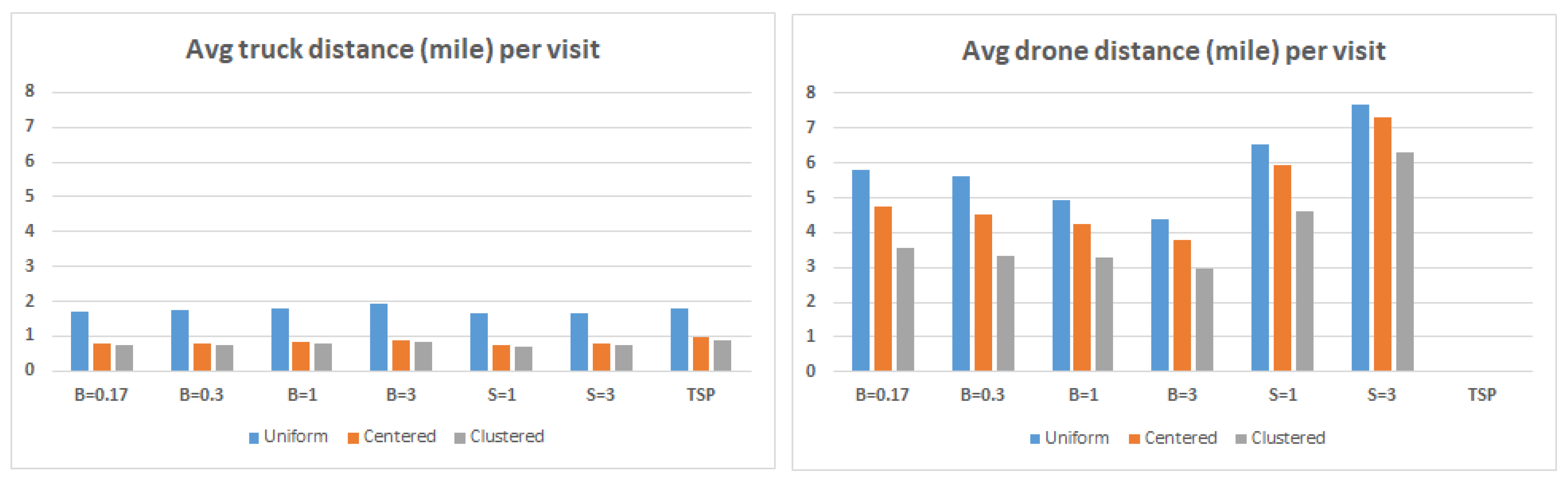
The carbon emissions for uniform data obtained under the recharging policy with varying charge speeds and the swapping policy with two different swap times are reported in Table 2. Each column represents a battery policy with the specified value for its distinctive parameter. For example, ‘R = 0.17’ provides the results under the recharging policy with a recharging rate of 0.17, whereas ‘S = 1’ implies the swapping policy where the battery is swapped in 1 min. We provide the truck’s emission in the first row, then the emission of the drone under varying energy requirements, AERDrone. The last column reports the best improvements among the six policies compared to the TSP emission. The total emission of the truck and the drone was considered for computing the improvements. According to the table, as the charge speed decreases in the recharging policy, the truck’s emission increases, whereas the drone’s emission decreases. This decrease is due to the distance traveled by the truck and the drone. The lower the charging speed, the longer it takes to reach the battery level required to perform subsequent flights. This leads to longer truck distances and shorter drone flights, as shown in Figure 16. Thus, the minimum emission is obtained with the fastest recharging. It is even better than the fast swapping policy. However, the difference is slight, nearly 1 kg. The slow swapping policy also emits less carbon than the slowest two recharging policies. It is clear that the emission increases as the energy requirement increases from 10 Wh/mi to 100 Wh/mi. However, it is still slight compared to the truck’s emission. When we examine the improvements obtained by deploying a drone in parcel delivery, we can conclude that nearly 25% less carbon is emitted.
When the customers are located around a center, they become closer, and the total distance decreases. This observation is verified by Figure 16. Since the truck and drone distances decrease, the emissions also decrease (Table 3). The truck’s emission is reduced to nearly half the amount emitted in the uniform data. The reduction in the TSP is similar. When the drone’s emission is compared to the uniform data, the reduction decreases from nearly 40% to 30% as the recharging is slower. Evaluating the six policies leads to results similar to those of the uniform data. The fastest recharging policy yields the lowest emissions. The second-fastest recharging policy is better than the slow swapping policy. The drone deployment provides nearly 30% lower emissions regarding the TSP.
Table 4 reports the emissions for clustered data. Since the customers are densely distributed around two distinct centers in networks of the same size, the distances are smaller relative to the centered data. The improvement against the TSP is nearly 30%. When recharging rates are 0.17 and 0.3, the recharging policy provides lower emissions than the swapping policy, which has a 1 min swapping time. The slow swapping policy is only better than the slowest recharging policy.
The uniform, centered, and clustered data results with 100 customers are provided in Table 5, Table 6 and Table 7, respectively. Regarding the battery policy, we can draw similar conclusions to those we obtained for 50 customers, with some exceptions. When there are 50 customers, the fastest recharging policy outperforms the swapping policy in all data types. However, the fast swapping policy provides lower emissions when the recharging rate is 0.3 and greater in the uniform and centered data. In the clustered data, the recharging policy is more sustainable even if the recharging rate is 0.3. When there are 100 customers, the two fastest recharging policies provide the lowest emissions in all data types, and the slowest two recharging policies are better than the slow swapping policy.
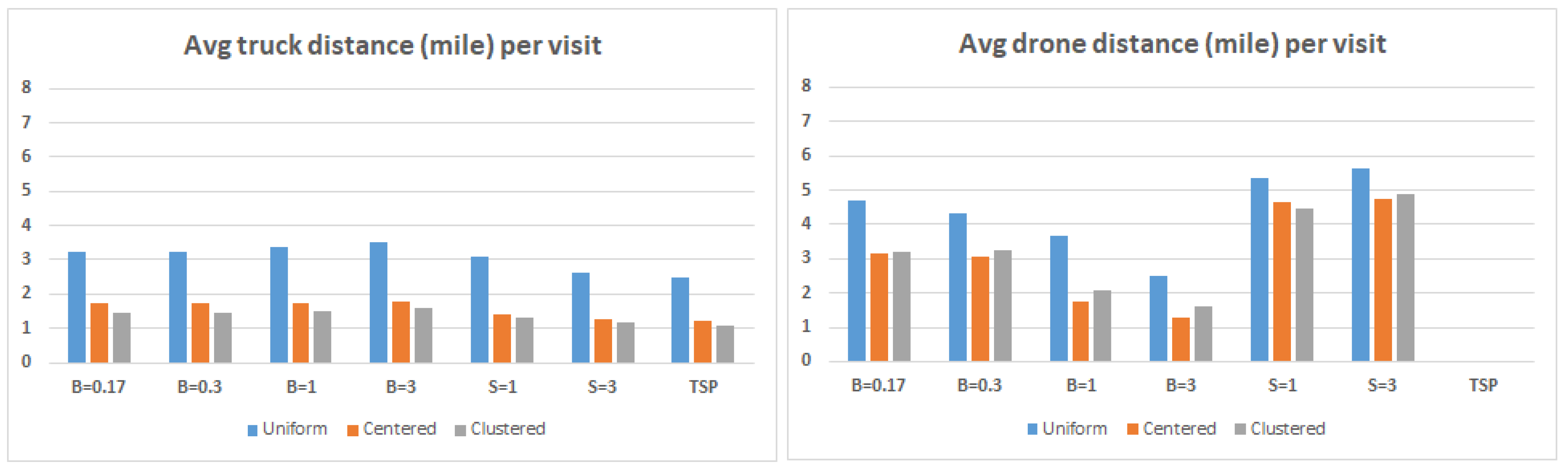
The deployment of the drone yields nearly 19% lower emissions than the TSP in all data types. The average improvements are smaller than those obtained for the 50-customer data, which are 25% for uniform data and 30% for the others. When we examine it in detail, we can see that as the number of customers increases from 50 to 100, the increase in emission by the TSP-D is greater than the increase by the TSP. The TSP emissions increase by 39%, 39%, and 41% for each data type, whereas the TSP-D emissions increase by 50%, 61%, and 61%. These results can be explained by Figure 17, which indicates that the average distance traveled per visit by the truck decreases as the recharging is faster, whereas the average distance traveled by the drone increases. When we compare it with the results obtained for 50-customer data (Figure 16), the average drone distance per visit is smaller, and the average truck distance per visit is greater for the 100-customer data. This yields a decrease in the improvement as the truck emits a significant amount of carbon.
5.3. Comparative Impact of Battery Policy on CO2 Emissions and Delivery Times
Es Yurek and Ozmutlu [19] reported that the swapping policy with a 1 min swapping time provided minimum delivery times when the customers are uniformly distributed. However, the fastest three recharging policies surpassed the swapping policy for the centered and clustered data. They analyzed the TSP-D under the recharging policy considering 10- and 20-customer instances. In this study, we ran our algorithm on 50- and 100-customer instances and came to a different conclusion. Table 8 provides the improvements against the TSP in delivery time and emission obtained for 50-customer data. According to the table, regarding the delivery time, the recharging policy surpasses the fast swapping policy with all recharging rates except the slowest one in all types of customer distribution. The slowest recharging also provides shorter delivery times than the slow swapping policy. This result is reasonable when we consider the number of drone nodes. Even when the swapping time is 1 min, the delivery time is extended by nearly 10 min in uniform data. The number of drone deliveries reduces as the recharging and the swapping slow down. This decrease leads to longer delivery times. When we examine the improvements in delivery time, we see that it explicitly decreases with slower recharging. Table 8 reports that the carbon emissions also follow the same trend. For example, for centered data, the improvement in delivery time was reduced by nearly 8% from the fastest recharging to the slowest. Similarly, the improvement in emissions was reduced by almost 8%. The results for the swapping policy are outstanding. For clustered data, the time improvement reduces by nearly 12% as the swapping slows from 1 min to 3 min. However, emission improvement reduced by nearly 5%. Because the time spent on battery swapping extends the delivery time but does not cause carbon emissions, it is clear that we should evaluate the battery policies considering both the delivery time and carbon emission.
Having conducted a comparative analysis, we can conclude that the recharging policy provides shorter delivery times and less carbon emissions when the recharging rate is 0.17 and 0.3. When the recharging rate is 1, the fast swapping policy provides lower emissions, whereas the recharging policy provides a shorter delivery time. Similarly, the slow swapping policy is more sustainable than the slowest recharging policy. In contrast, recharging is faster than swapping when the recharging rate is 3 and the swapping time is 3 min.
Table 9 provides the average improvements against TSP for 100-customer data and reports outstanding results. Like the above observations, the three fastest recharging policies yield shorter average delivery times than the fast swapping policy. Moreover, the slowest recharging policy is faster than the fast swapping policy when the customers are centered. The recharging policy yields lower emissions than the fast swapping policy when recharging is faster than discharging. However, the results reported for the average number of drone deliveries are remarkable. It increases in the centered and clustered data as the recharging becomes slower. Despite the increase in the number of drone deliveries, the average improvement in delivery time decreases by nearly 4% and 9%, respectively. When 100 customers are centered/clustered instead of 50 in an area of the same size, the density increases, and the customer nodes become closer. As the charging speed decreases, the drone is forced to visit customers within a short distance. Thus, the average number of drone deliveries increases in a densely populated network. Despite the increase in drone deliveries, the average improvement in time decreases because the total drone distance decreases.
6. Discussion
This study investigates the TSP-D from a sustainability perspective by comparing two battery policies: recharging and swapping. The recharging policy assumes that the drone is recharged simultaneously on top of the truck while the truck travels. It entails keeping track of the battery throughout the delivery because it increases or decreases depending on charge and discharge. We applied a simulated annealing algorithm to solve this problem and compute the emissions while minimizing the delivery time. As far as we know, this is the first study that addresses the carbon emissions of the TSP-D under the recharging policy.
Coordinated delivery provides better delivery and better sustainability performances. The improvement in TSP-D time is between nearly 2% and 20%, and the improvement in carbon emissions is between 9% and 21%. As the number of customers decreases from 100 to 50, the improvements against the TSP are greater. The recharging policy is better than the swapping policy regarding the delivery time and the emissions when the recharging is faster than discharging. This case is represented by two of four values specified for the recharging rate, 0.17 and 0.3. Moreover, it yields shorter delivery times when the battery is fully recharged within the battery life. The fast swapping policy provides lower emissions than the two slowest recharging policies. Additionally, it is faster than the slowest recharging policy. The slow swapping policy is the worst, considering both criteria. These results indicate that the TSP-D can be faster and more sustainable if the battery is recharged instead of being swapped. The battery should be fully charged within, at most, one-third of the discharge time to achieve this.
Although our experiments reveal that the TSP-D has the potential to improve the delivery and sustainability performances under the battery recharging policy, there are some limitations regarding the evaluation of carbon emissions. This study assumes that the battery life is consumed proportional to the distance traveled by the drone. However, in real life, other factors, such as drone speed and wind, affect the drone’s energy consumption. For example, the delivery performance improves as the drone travels faster, but this worsens energy consumption values. Similarly, wind speed and direction are other parameters that affect the drone’s battery consumption. Thus, speed-dependent energy consumption should be formulated as a further direction. Additionally, the wind factor should be considered. The realistic evaluation of energy consumption is significant in two aspects. First, energy consumption determines the drone range, which is one of the significant obstacles to the widespread use of delivery drones. Second, the drone’s carbon emission is evaluated considering the emission at the power generation facilities to recharge a lithium-ion battery, which depends on the energy consumption. In addition to including the accurate modeling of carbon emissions, this study could be extended to include multiple drones and trucks. Furthermore, allowing for multiple visits per flight may lead to challenging results regarding carbon emissions.
Funding
This research received no external funding.
Data Availability Statement
The data presented in this study are available on request from the corresponding author.
Conflicts of Interest
The author declares no conflict of interest.
References
- Top 10 Commercial Drone Delivery Companies. Available online: https://www.ecommercenext.org/top-10-commercial-drone-delivery-companies/ (accessed on 28 September 2022).
- Murray, C.C.; Chu, A. The flying sidekick traveling salesman problem: Optimization of drone-assisted parcel delivery. Transp. Res. Part C 2015, 54, 86–109. [Google Scholar] [CrossRef]
- Agatz, N.; Bouman, P.; Schmidt, M. Optimization approaches for the traveling salesman problem with drone. Transp. Sci. 2018, 52, 739–1034. [Google Scholar] [CrossRef]
- Es Yurek, E.; Ozmutlu, H.C. A decomposition-based iterative optimization algorithm for traveling salesman problem with drone. Transp. Res. Part C 2018, 91, 249–262. [Google Scholar] [CrossRef]
- Pugliese, L.; Macrina, G.; Guerriero, F. Trucks and drones cooperation in the last-mile delivery process. Networks 2020, 78, 371–399. [Google Scholar] [CrossRef]
- Coindreau, M.A.; Gallay, O.; Zufferey, N. Parcel delivery cost minimization with time window constraints using trucks and drones. Networks 2021, 78, 400–420. [Google Scholar] [CrossRef]
- Murray, C.C.; Raj, R. The multiple flying sidekick traveling salesman problem: Parcel delivery multiple drones. Transp. Res. Part C 2020, 110, 368–398. [Google Scholar] [CrossRef]
- Dell’Amico, M.; Montemanni, R.; Novellani, S. Modeling the flying sidekick traveling salesman problem with multiple drones. Networks 2021, 78, 303–327. [Google Scholar] [CrossRef]
- Sacramento, D.; Pisinger, D.; Ropke, S. An adaptive large neighborhood search metaheuristic for the vehicle routing problem with drones. Transp. Res. Part C 2019, 102, 289–315. [Google Scholar] [CrossRef]
- Kitjacharoenchai, P.; Ventresca, M.; Moshref-Javadi, M.; Lee, S.; Tanchoco, J.M.A.; Brunese, P.A. Multiple traveling salesman problem with drones: Mathematical model and heuristic approach. Comput. Ind. Eng. 2019, 129, 14–30. [Google Scholar] [CrossRef]
- Mahmoudi, B.; Eshghi, K. Energy-constrained multi-visit TSP with multiple drones considering non-customer rendezvous locations. Expert Syst. Appl. 2022, 210, 118479. [Google Scholar] [CrossRef]
- Xia, Y.; Zeng, W.; Zhang, C.; Yang, H. A branch-and-price-and-cut algorithm for the vehicle routing problem with load-dependent drones. Transp. Res. Part B 2023, 171, 80–110. [Google Scholar] [CrossRef]
- Marinelli, M.; Caggiani, L.; Ottomanelli, M.; Dell’Orco, M. En route truck–drone parcel delivery for optimal vehicle routing strategies. IET Intell. Transp. Syst. 2018, 12, 253–261. [Google Scholar] [CrossRef]
- Masone, A.; Poikonen, S.; Golden, B.L. The multivisit drone routing problem with edge launches: An iterative approach with discrete and continuous improvements. Networks 2022, 80, 193–215. [Google Scholar] [CrossRef]
- Eskandaripour, H.; Boldsaikhan, E. Last-mile drone delivery: Past, present, and future. Drones 2023, 7, 77. [Google Scholar] [CrossRef]
- Figliozzi, M.A. Lifecycle modeling and assessment of unmanned aerial vehicles (Drones) CO2 e emissions. Transp. Res. Part D 2017, 57, 251–261. [Google Scholar] [CrossRef]
- Goodchild, A.; Toy, J. Delivery by drone: An evaluation of unmanned aerial vehicle technology in reducing CO2 emissions in the delivery service industry. Transp. Res. Part D 2018, 61, 58–67. [Google Scholar] [CrossRef]
- Chiang, W.C.; Li, Y.; Shang, J.; Urban, T.L. Impact of drone delivery on sustainability and cost: Realizing the UAV potential through vehicle routing optimization. Appl. Energy 2019, 242, 1164–1175. [Google Scholar] [CrossRef]
- Es Yurek, E.; Ozmutlu, H.C. Traveling salesman problem with drone under recharging policy. Comput. Commun. 2021, 179, 35–49. [Google Scholar] [CrossRef]
- Tamke, F.; Buscher, U. The vehicle routing problem with drones and drone speed selection. Comput. Oper. Res. 2023, 152, 106112. [Google Scholar] [CrossRef]
- Vasquez, S.; Angulo, G.; Klapp, M.A. An exact solution method for the TSP with Drone based decomposition. Comput. Oper. Res. 2021, 127, 105127. [Google Scholar] [CrossRef]
- Bouman, P.; Agatz, N.; Schmidt, M. Dynamic programming approaches for the traveling salesman with drone. Networks 2018, 72, 528–542. [Google Scholar] [CrossRef]
- Dell’Amico, M.; Montemanni, R.; Novellani, S. Algorithms based on branch and bound for the flying sidekick traveling salesman problem. Omega 2021, 104, 102493. [Google Scholar] [CrossRef]
- Dell’Amico, M.; Montemanni, R.; Novellani, S. Exact models for the flying sidekick traveling salesman problem. Int. Trans. Oper. Res. 2022, 29, 1360–1393. [Google Scholar] [CrossRef]
- Dell’Amico, M.; Montemanni, R.; Novella, S. Drone-assisted deliveries: New formulations for the flying sidekick traveling salesman problem. Optim. Lett. 2021, 15, 1617–1648. [Google Scholar] [CrossRef]
- Boccia, M.; Masone, A.; Sforza, A.; Sterle, C. A column-and-row generation approach for the flying sidekick travelling salesman problem. Transp. Res. Part C 2021, 124, 102913. [Google Scholar] [CrossRef]
- Schermer, D.; Moeini, M.; Wendt, O. A branch-and-cut-approach and alternative formulations for the traveling salesman problem with drone. Networks 2020, 76, 164–186. [Google Scholar] [CrossRef]
- El-Adle, A.M.; Ghoniem, A.; Haouari, M. Parcel delivery by vehicle and drone. J. Oper. Res. Soc. 2021, 72, 398–416. [Google Scholar] [CrossRef]
- de Freitas, J.C.; Penna, P.H.V. A variable neighborhood search for flying sidekick traveling salesman problem. Int. Trans. Oper. Res. 2019, 27, 267–290. [Google Scholar] [CrossRef]
- Ha, Q.M.; Deville, Y.; Pham, Q.D.; Ha, M.H. A hybrid genetic algorithm for the traveling salesman problem with drone. J. Heuristics 2020, 26, 219–247. [Google Scholar] [CrossRef]
- Kundu, A.; Escobar, R.G.; Matis, T.I. An efficient routing heuristic for a drone-assisted delivery problem. IMA J. Manag. Math. 2021, 33, 583–601. [Google Scholar] [CrossRef]
- El-Adle, A.M.; Ghoniem, A.; Haouari, M. A variable neighborhood search for parcel delivery by vehicle with drone cycles. Comput. Oper. Res. 2023, 159, 106319. [Google Scholar] [CrossRef]
- Gunay-Sezer, N.S.; Cakmak, E.; Bulkan, S. A hybrid metaheuristic solution method to traveling salesman problem with drone. Systems 2023, 11, 259. [Google Scholar] [CrossRef]
- Liu, Z.; Li, X.; Khojandi, A. The flying sidekick traveling salesman problem with stochastic travel time: A reinforcement learning approach. Transp. Res. Part E 2022, 164, 102816. [Google Scholar] [CrossRef]
- Wang, X.; Poikonen, S.; Golden, B. The vehicle routing problem with drones: Several worst-case results. Optim. Lett. 2017, 11, 679–697. [Google Scholar] [CrossRef]
- Poikonen, S.; Wang, X.; Golden, B. The vehicle routing problem with drones: Extended models and connections. Networks 2017, 70, 34–43. [Google Scholar] [CrossRef]
- Thomas, T.; Srinivas, S.; Rajendran, C. Collaborative truck multi-drone delivery systems considering drone scheduling and en route operations. Ann. Oper. Res. 2023. [Google Scholar] [CrossRef]
- Moshref-Javadi, M.; Hemmati, A.; Winkenbach, M. A comparative analysis of synchronized truck-and-drone delivery models. Comput. Ind. Eng. 2021, 162, 107648. [Google Scholar] [CrossRef]
- Tiniç, G.O.; Karasan, O.E.; Kara, B.Y.; Campbell, J.E.; Ozel, A. Exact solution approaches for the minimum total cost traveling salesman problem with multiple drones. Transp. Res. Part B 2023, 168, 81–123. [Google Scholar] [CrossRef]
- Tamke, F.; Buscher, U. A branch-and-cut algorithm for the vehicle routing problem with drones. Transp. Res. Part B 2021, 144, 174–203. [Google Scholar] [CrossRef]
- Di Puglia Pugliese, L.; Guerriero, F. Last-Mile Deliveries by Using Drones and Classical Vehicles. In Optimization and Decision Science: Methodologies and Applications; Springer: Cham, Switzerland, 2017; pp. 557–565. [Google Scholar]
- Yin, Y.; Li, D.; Wang, D.; Ignatius, J.; Cheng, T.C.E.; Wang, S. A branch-and-price-and-cut algorithm for the truck-based drone delivery routing problem with time windows. Eur. J. Oper. Res. 2023, 309, 1125–1144. [Google Scholar] [CrossRef]
- Lei, D.; Cui, Z.; Li, M. A dynamical artificial bee colony for vehicle routing problem with drones. Eng. Appl. Artif. Intell. 2022, 107, 104510. [Google Scholar] [CrossRef]
- Kuo, R.J.; Lu, S.H.; Lai, P.Y.; Mara, S.T.W. Vehicle routing problem with drones considering time windows. Expert Syst. Appl. 2022, 191, 116264. [Google Scholar] [CrossRef]
- Li, H.; Chen, J.; Wang, F.; Zhao, Y. Truck and drone routing problem with synchronization on arcs. Networks 2022, 69, 884–901. [Google Scholar] [CrossRef]
- Luo, Z.; Gu, R.; Poon, M.; Liu, Z.; Lim, A. A last-mile drone-assisted one-to-one pickup and delivery problem with multi-visit drone trips. Comput. Oper. Res. 2022, 148, 106015. [Google Scholar] [CrossRef]
- Liu, Y.; Liu, Z.; Shi, J.; Wu, G.; Pedrycz, W. Two-echelon routing problem for parcel delivery by cooperated truck and delivery. IEEE Trans. Syst. Man Cybern. Syst. 2021, 51, 7450–7465. [Google Scholar] [CrossRef]
- Huang, S.H.; Huang, Y.H.; Blasquez, C.A.; Chen, C.Y. Solving the vehicle routing problem with drone for delivery services using an ant colony optimization algorithm. Adv. Eng. Inform. 2022, 51, 101536. [Google Scholar] [CrossRef]
- Meng, S.; Guo, X.; Li, D.; Liu, G. The multi-visit drone routing problem for pickup and delivery services. Transp. Res. Part E 2023, 169, 102990. [Google Scholar] [CrossRef]
- Campuzano, G.; Lall-Ruiz, E.; Mes, M. The drone-assisted variable speed asymmetric traveling salesman problem. Comput. Ind. Eng. 2023, 176, 109003. [Google Scholar] [CrossRef]
- Jeong, H.Y.; Song, B.D.; Lee, S. Truck-drone hybrid delivery routing: Payload-energy dependency and no-fly zones. Int. J. Prod. Econ. 2019, 214, 220–233. [Google Scholar] [CrossRef]
- Wu, G.; Mao, N.; Luo, Q.; Xu, B.; Shi, J.; Suganthan, P.N. Collaborative truck-drone routing for contacless parcel delivery during the epidemic. IEEE Trans. Intell. Transp. Syst. 2022, 23, 25077–25091. [Google Scholar] [CrossRef]
- Baldisseri, A.; Siragusa, C.; Seghezzi, A.; Mangiaracina, R.; Tumino, A. Truck-based drone delivery system: An economic and environmental assessment. Transp. Res. Part D 2022, 107, 103296. [Google Scholar] [CrossRef]
- Banyai, T. Impact of the integration of first-mile and last-mile drone-based operations from trucks and energy efficiency and the environment. Drones 2022, 6, 249. [Google Scholar] [CrossRef]
- Zhang, S.; Liu, S.; Xu, W.; Wang, W. A novel multi-objective optimization model for the vehicle routing problem with drone delivery and dynamic flight endurance. Comput. Ind. Eng. 2022, 173, 108679. [Google Scholar] [CrossRef]
- Baek, D.; Chen, Y.; Chang, N.; Macii, E.; Poncino, M. Energy-efficient coordinated electric truck-drone hybrid delivery service planning. In Proceedings of the 2020 AEIT International Conference of Electrical and Electronic Technologies for Automotive, Turin, Italy, 18–20 November 2020. [Google Scholar]
- Xiao, J.; Li, Y.; Cao, Z.; Xiao, J. Cooperative trucks and drones for rural last-mile delivery with steep roads. Comput. Ind. Eng. 2024, 187, 109849. [Google Scholar] [CrossRef]
- Kirkpatrick, S.; Gelatt, C.D.; Vecchi, M.P. Optimization by simulated annealing. Science 1983, 220, 671–680. [Google Scholar] [CrossRef] [PubMed]
Figure 1.
An illustrative example of the TSP-D.

Figure 2.
An illustrative example of the solution vector.

Figure 3.
An illustrative example of the tour vector.

Figure 4.
The TSP-D solution after swap_in().

Figure 5.
The TSP-D solution after swap_cross().

Figure 6.
The TSP-D solution after swap_out().

Figure 7.
Three cases in swap_position().

Figure 8.
The TSP-D solution after swap_position().

Figure 9.
The TSP-D solution after relocating a truck-only node as an in-tandem node.

Figure 10.
The TSP-D solution after relocating a truck-only node in another tour as a truck-only node.
Figure 10.
The TSP-D solution after relocating a truck-only node in another tour as a truck-only node.

Figure 11.
Illustrative examples for relocate_out().

Figure 12.
The TSP-D solution after the insertion of an in-tandem node.

Figure 13.
The TSP-D solution after the insertion of a tour.

Figure 14.
The TSP-D solution after group().

Figure 15.
The TSP-D solution after destroy.

Figure 16.
Comparison of average distance per visit traveled by the truck and the drone for 50-customer data.
Figure 16.
Comparison of average distance per visit traveled by the truck and the drone for 50-customer data.

Figure 17.
Comparison of average distance per visit traveled by the truck and the drone for 100-customer data.
Figure 17.
Comparison of average distance per visit traveled by the truck and the drone for 100-customer data.


Table 1.
Comparison of the heuristic performance with the performance of the reference study.
| Uniform Data | Centered Data | Clustered Data | |||||||
|---|---|---|---|---|---|---|---|---|---|
| Battery Policy | Benchmark Study [19] | This Study | Imp (%) | Benchmark Study [19] | This Study | Imp (%) | Benchmark Study [19] | This Study | Imp (%) |
| R = 0.17 | 103.10 | 102.09 | −0.98 | 59.70 | 59.02 | −1.14 | 49.27 | 48.84 | −0.87 |
| R = 0.33 | 103.50 | 10296 | −0.52 | 50.32 | 51.27 | 1.89 | 49.27 | 48.55 | −1.46 |
| R = 1 | 108.22 | 107.06 | −1.07 | 52.03 | 51.02 | −1.94 | 50.41 | 49.03 | −2.74 |
| R = 3 | 117.12 | 113.06 | −3.47 | 55.37 | 53.17 | −3.97 | 52.93 | 50.08 | −5.38 |
| S = 1 | 104.29 | 106.93 | 2.53 | 52.28 | 52.02 | −0.50 | 53.99 | 53.16 | −1.54 |
| S = 3 | 115.69 | 118.07 | 2.06 | 58.33 | 58.21 | −0.21 | 60.38 | 59.75 | −1.04 |
Table 2.
Carbon emissions (Kg) for uniform data with 50 customers.
| AERDrone (Wh/mi) | R = 0.17 | R = 0.3 | R = 1 | R = 3 | S = 1 | S = 3 | TSP | Best Imp % | |
|---|---|---|---|---|---|---|---|---|---|
| Emission of Truck | 83.03 | 84.81 | 88.48 | 93.82 | 84.22 | 86.56 | 112.69 | ||
| Emission of Drone | 10 | 0.24 | 0.23 | 0.18 | 0.12 | 0.25 | 0.24 | 26.10 | |
| 20 | 0.49 | 0.46 | 0.36 | 0.25 | 0.50 | 0.48 | 25.89 | ||
| 30 | 0.73 | 0.69 | 0.54 | 0.37 | 0.74 | 0.72 | 25.67 | ||
| 40 | 0.97 | 0.92 | 0.71 | 0.49 | 0.99 | 0.95 | 25.46 | ||
| 50 | 1.22 | 1.14 | 0.89 | 0.62 | 1.24 | 1.19 | 25.24 | ||
| 60 | 1.46 | 1.37 | 1.07 | 0.74 | 1.49 | 1.43 | 25.02 | ||
| 70 | 1.70 | 1.60 | 1.25 | 0.87 | 1.73 | 1.67 | 24.81 | ||
| 80 | 1.95 | 1.83 | 1.43 | 0.99 | 1.98 | 1.91 | 24.59 | ||
| 90 | 2.19 | 2.06 | 1.61 | 1.11 | 2.23 | 2.15 | 24.38 | ||
| 100 | 2.43 | 2.29 | 1.79 | 1.24 | 2.48 | 2.38 | 24.16 | ||
| Total emission (min) | 10 | 83.27 | 85.04 | 88.66 | 93.94 | 84.47 | 86.80 | 112.69 | 26.10 |
| Total emission (max) | 100 | 85.46 | 87.09 | 90.27 | 95.06 | 86.70 | 88.95 | 112.69 | 24.16 |
Table 3.
Carbon emissions (Kg) for centered data with 50 customers.
| AERDrone (Wh/mi) | R = 0.17 | R = 0.3 | R = 1 | R = 3 | S = 1 | S = 3 | TSP | Best Imp % | |
|---|---|---|---|---|---|---|---|---|---|
| Emission of Truck | 41.23 | 41.77 | 43.73 | 46.39 | 41.64 | 43.22 | 60.83 | ||
| Emission of Drone | 10 | 0.14 | 0.13 | 0.11 | 0.09 | 0.15 | 0.14 | 31.99 | |
| 20 | 0.28 | 0.27 | 0.22 | 0.18 | 0.29 | 0.28 | 31.76 | ||
| 30 | 0.43 | 0.40 | 0.34 | 0.27 | 0.44 | 0.43 | 31.52 | ||
| 40 | 0.57 | 0.53 | 0.45 | 0.35 | 0.59 | 0.57 | 31.29 | ||
| 50 | 0.71 | 0.66 | 0.56 | 0.44 | 0.74 | 0.71 | 31.06 | ||
| 60 | 0.85 | 0.80 | 0.67 | 0.53 | 0.88 | 0.85 | 30.83 | ||
| 70 | 0.99 | 0.93 | 0.78 | 0.62 | 1.03 | 0.99 | 30.59 | ||
| 80 | 1.13 | 1.06 | 0.90 | 0.71 | 1.18 | 1.14 | 30.36 | ||
| 90 | 1.28 | 1.19 | 1.01 | 0.80 | 1.33 | 1.28 | 30.13 | ||
| 100 | 1.42 | 1.33 | 1.12 | 0.89 | 1.47 | 1.42 | 29.89 | ||
| Total min | 10 | 41.37 | 41.90 | 43.84 | 46.48 | 41.79 | 43.36 | 60.83 | 31.99 |
| Total max | 100 | 42.65 | 43.10 | 44.85 | 47.28 | 43.12 | 44.64 | 60.83 | 29.89 |
Table 4.
Carbon emissions (Kg) for clustered data with 50 customers.
| AERDrone (Wh/mi) | R = 0.17 | R = 0.3 | R = 1 | R = 3 | S = 1 | S = 3 | TSP | Best Imp % | |
|---|---|---|---|---|---|---|---|---|---|
| Emission of Truck | 37.43 | 37.79 | 39.28 | 41.48 | 38.38 | 41.01 | 55.08 | ||
| Emission of Drone | 10 | 0.12 | 0.12 | 0.10 | 0.08 | 0.13 | 0.12 | 31.82 | |
| 20 | 0.25 | 0.24 | 0.20 | 0.16 | 0.25 | 0.24 | 31.59 | ||
| 30 | 0.37 | 0.35 | 0.31 | 0.24 | 0.38 | 0.35 | 31.37 | ||
| 40 | 0.49 | 0.47 | 0.41 | 0.33 | 0.51 | 0.47 | 31.15 | ||
| 50 | 0.62 | 0.59 | 0.51 | 0.41 | 0.64 | 0.59 | 30.92 | ||
| 60 | 0.74 | 0.71 | 0.61 | 0.49 | 0.76 | 0.71 | 30.70 | ||
| 70 | 0.86 | 0.82 | 0.72 | 0.57 | 0.89 | 0.82 | 30.47 | ||
| 80 | 0.99 | 0.94 | 0.82 | 0.65 | 1.02 | 0.94 | 30.25 | ||
| 90 | 1.11 | 1.06 | 0.92 | 0.73 | 1.14 | 1.06 | 30.02 | ||
| 100 | 1.24 | 1.18 | 1.02 | 0.82 | 1.27 | 1.18 | 29.80 | ||
| Total min | 10 | 37.55 | 37.91 | 39.38 | 41.56 | 38.50 | 41.12 | 55.08 | 31.82 |
| Total max | 100 | 38.67 | 38.97 | 40.30 | 42.29 | 39.65 | 42.18 | 55.08 | 29.80 |
Table 5.
Carbon emissions (Kg) for uniform data with 100 customers.
| AERDrone (Wh/mi) | R = 0.17 | R = 0.3 | R = 1 | R = 3 | S = 1 | S = 3 | TSP | Best Imp % | |
|---|---|---|---|---|---|---|---|---|---|
| Emission of Truck | 124.08 | 125.48 | 129.90 | 135.74 | 127.03 | 136.16 | 156.58 | 20.75 | |
| Emission of Drone | 10 | 0.34 | 0.31 | 0.24 | 0.15 | 0.35 | 0.21 | 20.54 | |
| 20 | 0.67 | 0.62 | 0.48 | 0.30 | 0.69 | 0.41 | 20.33 | ||
| 30 | 1.01 | 0.93 | 0.72 | 0.44 | 1.04 | 0.62 | 20.11 | ||
| 40 | 1.35 | 1.25 | 0.95 | 0.59 | 1.38 | 0.82 | 19.90 | ||
| 50 | 1.68 | 1.56 | 1.19 | 0.74 | 1.73 | 1.03 | 19.68 | ||
| 60 | 2.02 | 1.87 | 1.43 | 0.89 | 2.07 | 1.23 | 19.46 | ||
| 70 | 2.36 | 2.18 | 1.67 | 1.04 | 2.42 | 1.44 | 19.25 | ||
| 80 | 2.69 | 2.49 | 1.91 | 1.18 | 2.76 | 1.64 | 19.03 | ||
| 90 | 3.03 | 2.80 | 2.15 | 1.33 | 3.11 | 1.85 | 18.82 | ||
| 100 | 3.37 | 3.12 | 2.38 | 1.48 | 3.46 | 2.05 | 18.60 | ||
| Total min | 10 | 124.42 | 125.79 | 130.14 | 135.89 | 127.38 | 136.37 | 156.58 | 20.54 |
| Total max | 100 | 127.45 | 128.59 | 132.28 | 137.22 | 130.49 | 138.22 | 156.58 | 18.60 |
Table 6.
Carbon emissions (Kg) for centered data with 100 customers.
| AERDrone (Wh/mi) | R = 0.17 | R = 0.3 | R = 1 | R = 3 | S = 1 | S = 3 | TSP | Best Imp % | |
|---|---|---|---|---|---|---|---|---|---|
| Emission of Truck | 66.84 | 67.33 | 68.05 | 69.82 | 67.88 | 73.38 | 84.41 | 20.82 | |
| Emission of Drone | 10 | 0.20 | 0.18 | 0.13 | 0.10 | 0.19 | 0.08 | 20.59 | |
| 20 | 0.39 | 0.36 | 0.26 | 0.19 | 0.39 | 0.15 | 20.36 | ||
| 30 | 0.59 | 0.54 | 0.40 | 0.29 | 0.58 | 0.23 | 20.13 | ||
| 40 | 0.78 | 0.71 | 0.53 | 0.39 | 0.78 | 0.30 | 19.89 | ||
| 50 | 0.98 | 0.89 | 0.66 | 0.48 | 0.97 | 0.38 | 19.66 | ||
| 60 | 1.17 | 1.07 | 0.79 | 0.58 | 1.16 | 0.45 | 19.43 | ||
| 70 | 1.37 | 1.25 | 0.93 | 0.68 | 1.36 | 0.53 | 19.20 | ||
| 80 | 1.56 | 1.43 | 1.06 | 0.77 | 1.55 | 0.61 | 18.97 | ||
| 90 | 1.76 | 1.61 | 1.19 | 0.87 | 1.75 | 0.68 | 18.74 | ||
| 100 | 1.95 | 1.79 | 1.32 | 0.97 | 1.94 | 0.76 | 18.51 | ||
| Total min | 10 | 67.03 | 67.50 | 68.19 | 69.92 | 68.07 | 73.46 | 84.41 | 20.59 |
| Total max | 100 | 68.79 | 69.11 | 69.38 | 70.79 | 69.82 | 74.14 | 84.41 | 18.51 |
Table 7.
Carbon emissions (Kg) for clustered data with 100 customers.
| AERDrone (Wh/mi) | R = 0.17 | R = 0.3 | R = 1 | R = 3 | S = 1 | S = 3 | TSP | Best Imp % | |
|---|---|---|---|---|---|---|---|---|---|
| Emission of Truck | 61.19 | 61.88 | 64.09 | 67.81 | 62.35 | 70.68 | 77.65 | 21.19 | |
| Emission of Drone | 10 | 0.19 | 0.18 | 0.13 | 0.09 | 0.20 | 0.05 | 20.94 | |
| 20 | 0.39 | 0.36 | 0.26 | 0.19 | 0.40 | 0.11 | 20.69 | ||
| 30 | 0.58 | 0.54 | 0.39 | 0.28 | 0.59 | 0.16 | 20.44 | ||
| 40 | 0.78 | 0.73 | 0.52 | 0.37 | 0.79 | 0.22 | 20.19 | ||
| 50 | 0.97 | 0.91 | 0.66 | 0.46 | 0.99 | 0.27 | 19.94 | ||
| 60 | 1.16 | 1.09 | 0.79 | 0.56 | 1.19 | 0.33 | 19.70 | ||
| 70 | 1.36 | 1.27 | 0.92 | 0.65 | 1.39 | 0.38 | 19.45 | ||
| 80 | 1.55 | 1.45 | 1.05 | 0.74 | 1.58 | 0.44 | 19.20 | ||
| 90 | 1.74 | 1.63 | 1.18 | 0.84 | 1.78 | 0.49 | 18.95 | ||
| 100 | 1.94 | 1.82 | 1.31 | 0.93 | 1.98 | 0.55 | 18.70 | ||
| Total min | 10 | 61.39 | 62.06 | 64.22 | 67.90 | 62.54 | 70.74 | 77.65 | 20.94 |
| Total max | 100 | 63.13 | 63.70 | 65.40 | 68.73 | 64.33 | 71.23 | 77.65 | 18.70 |
Table 8.
Comparative analysis of carbon emissions and delivery times regarding battery policies and customer distributions for 50-customer data.
Table 8.
Comparative analysis of carbon emissions and delivery times regarding battery policies and customer distributions for 50-customer data.
| Customer Density | R = 0.17 | R = 0.3 | R = 1 | R = 3 | S = 1 | S = 3 | |
|---|---|---|---|---|---|---|---|
| Avg. number of drone nodes | uniform | 11.14 | 10.81 | 9.65 | 7.53 | 10.06 | 8.28 |
| centered | 8.16 | 8.16 | 7.37 | 6.58 | 6.66 | 5.18 | |
| clustered | 9.52 | 9.99 | 8.70 | 7.66 | 7.41 | 4.99 | |
| Avg. imp. (%) in delivery time against TSP | uniform | 24.73 | 23.94 | 20.53 | 15.71 | 19.90 | 11.30 |
| centered | 30.84 | 30.14 | 27.04 | 22.81 | 24.98 | 15.20 | |
| clustered | 30.85 | 30.04 | 27.39 | 23.70 | 22.63 | 11.07 | |
| Avg. imp. (%) in CO2 emission against TSP | uniform | 26.10 | 24.54 | 21.33 | 16.64 | 25.04 | 22.97 |
| centered | 31.99 | 31.11 | 27.93 | 23.59 | 31.30 | 28.72 | |
| clustered | 31.82 | 31.17 | 28.50 | 24.55 | 30.09 | 25.33 |
Table 9.
Comparative analysis of carbon emissions and delivery times regarding battery policies and customer distributions for 100-customer data.
Table 9.
Comparative analysis of carbon emissions and delivery times regarding battery policies and customer distributions for 100-customer data.
| Customer Density | R = 0.17 | R = 0.3 | R = 1 | R = 3 | S = 1 | S = 3 | |
|---|---|---|---|---|---|---|---|
| Avg. number of drone nodes | uniform | 19.21 | 19.25 | 17.58 | 16.68 | 17.42 | 8.84 |
| centered | 18.44 | 17.82 | 23.12 | 22.03 | 11.08 | 3.71 | |
| clustered | 16.22 | 15.01 | 18.94 | 19.50 | 11.79 | 2.71 | |
| Avg. % imp. in delivery time against TSP | uniform | 19.80 | 18.82 | 15.94 | 11.81 | 12.92 | 3.79 |
| centered | 18.76 | 18.44 | 16.68 | 14.52 | 11.54 | 4.25 | |
| clustered | 19.97 | 19.10 | 15.81 | 10.99 | 11.07 | 2.47 | |
| Avg. % imp. CO2 emission against TSP | uniform | 20.54 | 19.66 | 16.89 | 13.21 | 18.65 | 12.91 |
| centered | 20.59 | 20.03 | 19.22 | 17.17 | 19.36 | 12.98 | |
| clustered | 20.94 | 20.07 | 17.29 | 12.55 | 19.45 | 8.90 |
Disclaimer/Publisher’s Note: The statements, opinions and data contained in all publications are solely those of the individual author(s) and contributor(s) and not of MDPI and/or the editor(s). MDPI and/or the editor(s) disclaim responsibility for any injury to people or property resulting from any ideas, methods, instructions or products referred to in the content. |
© 2024 by the author. Licensee MDPI, Basel, Switzerland. This article is an open access article distributed under the terms and conditions of the Creative Commons Attribution (CC BY) license (https://creativecommons.org/licenses/by/4.0/).
Share and Cite
MDPI and ACS Style
Es Yurek, E. Impact of Drone Battery Recharging Policy on Overall Carbon Emissions: The Traveling Salesman Problem with Drone. Drones 2024, 8, 108. https://0-doi-org.brum.beds.ac.uk/10.3390/drones8030108
AMA Style
Es Yurek E. Impact of Drone Battery Recharging Policy on Overall Carbon Emissions: The Traveling Salesman Problem with Drone. Drones. 2024; 8(3):108. https://0-doi-org.brum.beds.ac.uk/10.3390/drones8030108
Chicago/Turabian StyleEs Yurek, Emine. 2024. "Impact of Drone Battery Recharging Policy on Overall Carbon Emissions: The Traveling Salesman Problem with Drone" Drones 8, no. 3: 108. https://0-doi-org.brum.beds.ac.uk/10.3390/drones8030108