Condition Monitoring of Manufacturing Processes under Low Sampling Rate


1
Polytechnique Montreal, Montréal, QC H3T 1J4, Canada
2
Howmet Aerospace, Pittsburgh, PA 15213, USA
*
Author to whom correspondence should be addressed.
†
Current address: 2500, Chemin de Polytechnique Montréal, Québec, QC H3T 1J4, Canada.
‡
These authors contributed equally to this work.
J. Manuf. Mater. Process. 2021, 5(1), 26; https://0-doi-org.brum.beds.ac.uk/10.3390/jmmp5010026
Submission received: 23 February 2021
/
Revised: 19 March 2021
/
Accepted: 19 March 2021
/
Published: 23 March 2021
(This article belongs to the Special Issue Application of Data-Driven Methods for Material Science and Manufacturing Processes)
Abstract
:Manufacturing processes can be monitored for anomalies and failures just like machines, in condition monitoring and prognostic and health management. This research takes inspiration from condition monitoring and prognostic and health management techniques to develop a method for part production process monitoring. The contribution brought by this paper is an automated technique for process monitoring that works with low sampling rates of , a limitation that comes from using data provided by an industrial partner and acquired from industrial manufacturing processes. The technique uses kernel density estimation functions on machine tools spindle load historical time signals for distribution estimation. It then uses this estimation to monitor the manufacturing processes for anomalies in real time. A modified version was tested by our industrial partner on a titanium part manufacturing line.

1. Introduction
Condition-based monitoring (CBM) is defined as the act of monitoring the condition of a machine or a process [1], while prognostics and health management (PHM) is defined as an algorithmic way of detecting, predicting, monitoring and assessing operation problems and health changes of systems [2] as well as taking decisions on them. Both are used to monitor machinery, such as pumps [3], bearings and gears [4,5], electronics [6], plane parts [6] and machine tools (Computer Numerical Control (CNC)) [2,7]. This field of research is backed by a strong interest of the industry towards Smart Manufacturing, also called Industry 4.0, which aims at the autonomous management of production through virtualization of the production chain [8]. This is mainly achieved through the effective leverage of advances in the Internet of Things (IoT) [9] and Big Data analytics [10] technologies. Moreover, when used for monitoring purposes, CBM and PHM can be used to optimize the part production process, reduce costs and increase yields.
CBM and PHM research is split in two main research categories, namely model-based approaches [1,11] and data-oriented approaches [1,12]. Model-based approaches need expert knowledge of the system to be built and are dedicated to that system, as presented in [11], where a finite element model of the system for prognostic and health management is developed. Data-oriented approaches are more abstract. They use data acquired on the system and knowledge of the outcome to build a model representing the phenomenon [12]. For example, Zhang et al. [13] show how a deep convolutional neural network trained on a vibration temporal signal can predict bearing faults. They only use the input data, vibration over time, and output information, and a vector of size 10 used as a voting method, to classify the four bearings’ states. These methods are of great interest since they can be updated easily without expert knowledge of the machine and can be trained to work on more than one system, as long as good quality contextual data are available.
Additionally, process monitoring research still focuses on design, as highlighted by the review of Imad et al. [14], Hopkins and Hosseini [15]. Lu et al. [16] review the deployment of the STEP-NC standard for a CNC system programming interface that enables bi-directional communication between machine tool controllers, computer-aided design (CAD)/Computer-Aided Manufacturing (CAM) software, monitoring software, etc. Unfortunately, Lu et al. [16] reveal that most CNC controller vendors are not compliant with the standard. The authors also state that STEP-NC could be used for cloud manufacturing frameworks, such as the ones presented by Caggiano [17] or Siddhartha et al. [18], but manufacturers seem reluctant to the use of this open standard citing legacy machine compatibility problems for older machines and the high cost of early adoption, hindering development in this field. CNC manufacturers, as well as the machining industry, are slowly integrating more digital options in their systems, but it is not yet clear whether they will transition to open technologies that will help research in the CBM and PHM fields or to closed source solutions sold by the CNC manufacturers themselves when it comes to machine condition and process monitoring. This makes building a decision making system challenging since CNC manufacturers tend to use their own closed-source system for accessing the CNC controller’s functionalities.
This paper proposes a data-driven automated system for normal behavior signal determination applied to the manufacturing process of complex aerospace parts with a low sampling rate, limited to by our industrial partner who could not change this setting. The technology used in our approach is kernel density estimation functions [19]. The advantages of solutions using a low sampling rate are the speed of numerical computations and the small amount of data storage required to keep historical data for testing or even further improvements of the algorithms. First, the paper discusses previous work in this field. Then, the data used in this study for process monitoring research, which were acquired by industry, are detailed. The data are complex and demonstrate the challenges faced by companies transitioning towards Industry 4.0 for process monitoring. We then present an explanation of the processing needed for normal behavior determination by using kernel density estimation functions and the results. A discussion on how the method can be used for monitoring and its limitations ensues. Finally, a practical implementation of this technology is presented and discussed at the end of this paper.
2. Materials and Methods
In the field of CBM and PHM, research is performed on high frequency acquisition rates. Jin et al. [20] proposed a method for bearing fault prognosis using a derivation of wavelet transform as a health index and tested on a dataset acquired at 25.6 kHZ. Rafiee et al. [21] proposed a method based on neural networks for gearbox condition monitoring and tested their approach on a dataset acquired at 16,384 . Bhuiyan et al. [22] studied acoustic emission, and the lowest acquisition rate studied was 50 kHZ. Rivero et al. [23] proposed a method based on time domain analysis of cutting power and axial cutting force. The proposed approach was able to predict variability in the acquired signal corresponding to tool wear. The frequency used for the signal acquisition was in the range of 500–1500 kHZ. Zhang et al. [24] used kernel density estimation (KDE) and and Kullback–Leibler divergence to monitor rotating machinery. Their work was shown to outperform both support-vector machine and neural network-based approaches on data sampled at 20 kHZ. Lee et al. [25] used KDE to monitor tool wear using by using T2-statistics and Q-statistics with control charts. They used NASA’s milling dataset [26] for which data were acquired at a minimum of 100 kHZ. It is hard to find, in the scientific literature, methods of monitoring CNC machine tools’ behaviors on low sampling rate data.
This is a problem, since our industrial partner acquires data from its machines at a limited sampling rate of .
KDE functions are used to approximate the probability density function of random variables [27]. The function is very fast to compute and can reliably model multi-modal distributions [27]. KDE was used by the authors in the data exploration phase and was proven to reliably model the underlying dataset.
For all the abovementioned reasons, this paper focuses on a condition monitoring method that can be used on low sampling rate data by using KDE functions.
2.1. Dataset
Our industrial partner acquires data on there shop floors from all machines that produce data and from three main sources. First, the controller of the machines; second, a spindle assisted program that monitors the use time of tools; and third, the advance spindle technology software for their machines, which gives information about the spindle state, such as spindle power, spindle torque, axial force min, axial force max, etc. They save all of this information at a rate of , whether the machines are running or not. This is a hard limitation of their system. This study focuses on our industrial partner’s titanium production line. This choice was motivated by the fact that more data are available through the controller of the machines used on these production lines and it was in the interest of our industrial partner to make this research since their cost of operation is high and any down time results in high loss in revenue.
Figure 1 shows that, for each part produced, there are multiple operations needed on the raw material (pre-forged titanium). All of these operations are represented by programs. Those programs can run multiple times on the machines each time the part needs to be produced. Then all programs are divided into sub-programs that represent the geometrical features of the part. Additionally, each sub-program, and by extension program, uses different tools to produce the different features of the part. Finally, while in production, sensors are used to monitor the whole process.
2.2. Sensors
The sensors used were installed on the machines by the CNC manufacturer. In terms of sensors, Table 1 shows the different categories of data acquired by the machine’s controller. This data contain all necessary information to identify the running CNC program, tools and sub-programs. This information is saved in a database following the structure shown by Figure 2. This is necessary for data analysis since different operations and different tools result in very different signals acquired.
One of the major challenges with the built data base is that the data are not synchronized. As explained, a CNC machining program is comprised of multiple sub-programs that can directly be associated with geometrical features of the part to be machined, see Figure 2. These sub-programs are generated by computer-aided design (CAD) software (CATIA, Solid Work, etc.). At the change of each sub-program, the machining process may use a different tool, or the new sub-program may correspond to a new geometry. Moreover, even if the same tool model is used between two sub-programs, G-Code programmers may ask for a tool change, also called the use of a sister tool, to ensure the quality of the cutting process. These must all be taken into account when building a model for process monitoring using data acquired in production settings. Finally, for all changes of sub-programs, there is a possibility of inducing a delay due to uncertainty between the loading time of the next sub-program and the variability of tool change times. Those delays cause problems since the goal is to treat the data acquired as time series that can be statistically compared with each other. Each delay must be removed and all time series must be properly synchronized with each other. This means that the timestamp of the acquisition cannot be used for accurate comparison.
2.3. Data Processing
As shown in Table 1, one of the signals acquired by the machine tools’ controllers is the Spindle Load. The spindle load is given in % and represents the force needed to keep the tool rotating at the desired speed with respect to the maximum amount of force the motor can exert. On 28 February 2018, a catastrophic breakage occurred and a part was scrapped. The spindle load signal acquired for this particular event compared with historical production of the same part is shown in Figure 3. It is clear visually that the signal acquired was off with respect to historical runs; see red circle and arrow. Other signals, such as the vibration registered for the same event, were also off; however, this research will focus solely on the spindle load.
2.4. Data Synchronization
Figure 4 shows the raw spindle load data acquired for 18 runs of the same process. The run number is a label that represents a CNC program, a tool and the time it was run. The label number 127 represents a run made on 2018-10-13T21:08:57-04:00 while the program number 356 was run on 2018-11-16T8:58:31-05:00. By analyzing this figure, where data where synchronized using Algorithm 1 to reduce variations within all runs, it is still hard to determine if all data points correspond perfectly to the position in time to which they were attributed due to noise in the data acquisition. For comparison, Figure 5 shows a single run of this program, the run labeled 127.
| Algorithm 1: Program run synchronization |
 |
Nonetheless, the data in Figure 4 and Figure 5 are concentrated in a band. There is a starting upward phase where the spindle load is increasing rapidly while the CNC machine is trying to keep the tool’s rotation at the desired speed while it starts cutting titanium. Then there is a series of ups and downs until the end of the operation. Such a behavior can be automatically extracted and quantified using the techniques presented in this paper.
2.5. Kernel Density Estimation
This section discusses how kernel density estimation (KDE) functions can be used to automatically capture the pattern in historical runs, and exemplified by the runs in Figure 4. Since CNC machine tools are highly repeatable machines [28], it is expected that two runs of the same program should yield very similar results (i.e., be repeatable). For such a repeatable processes, knowing the region in space where the data should be can be used for monitoring purposes.
KDE is used to estimate the probability density of a dataset, in order to find where most of the data is situated in a certain space. For this study, the “space” is the spindle load.
Equation (1) [27] is the KDE function estimated by the points (x) in our dataset and where is the estimated probability density function, K is the kernel used for the estimation, n is the number of points in the dataset and h is the bandwidth, which serves as a smoothing parameter. To automate the bandwidth selection, the method proposed by Sheather and Jones [29] was used.
Since the goal is to compare the current part production process with the known normal behavior run of the same production program, we can use KDE on the measured signals to estimate what values are the most probable. Computing an estimation of the probability density function of spindle loads yields an idea regarding which values are most commonly measured to test if the program run replicates the same behavior.
2.6. Normal Behavior Computation
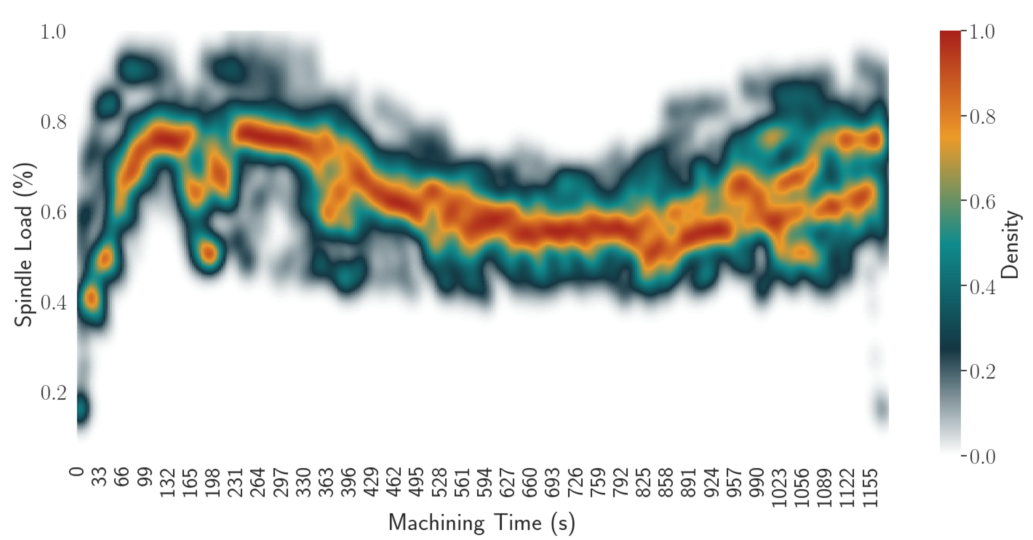
To determine the normal behavior of a program, the KDE is computed on the spindle load signal for bins of 3 s corresponding to the sampling rate of our data acquisition system (see Algorithm 2). This gives the region in space where the largest amount of data can be found for each time bin, i.e., the density function of spindle load for each time bin. Figure 6 illustrates this density with a heat map where the color represents the density score for each time bin (abscissa) and each spindle value (ordinate) computed on the 15 historical runs shown in Figure 4. Figure 6’s color map goes from 0 to 1 because it was normalized with respect to the maximum density score of each time bin (see Algorithm 3). In accordance with Figure 4, the white region shows where the KDE computation estimates that the density score is 0 and all of the colored region is where data were found. Furthermore, the estimated density for each time bin and spindle load value gives an insight of what represents a normal behavior of a machining program. The closer to 1 is the density score for a spindle load value and time bin combination, the more it is considered normal.
| Algorithm 2: Computation of KDEs for each time bin |
 |
| Algorithm 3: Heat map computation |
 |
3. Results
With the visualization of Figure 6 extracted from Algorithm 2, monitoring of future runs of the same sub-program and tool is possible. Indeed, KDEs enable us to compute a score for a combination of time bin and spindle load value. If this score is near 1, that means the probability of seeing this value is high, whereas if the score is near 0, then the probability of seeing this value is low. A succession of unexpected values means there is a problem with the machining program.
3.1. CNC Program Normal Behavior
The normal behavior computation of a part of a CNC program is given in Figure 7. The light blue region shows the normal behavior area of the program and all the runs of Figure 4 are shown on top. The more runs there are about the process, the more precise the computation is, since the estimate of the underlying distribution given by the KDE will be more accurate [27]. To extract the normal behavior, the data used to compute the model must come from runs where the process was considered normal.
To extract the visualization presented in Figure 7, the result of Algorithm 3, a heat map computation, was treated as probabilities and any value under was removed to generate the blue region of Figure 7. This threshold was chosen based on the aforementioned hypothesis that machine tools are highly repeatable. Thus, the score given by the kernel density estimation and represented in Figure 6 by the density bar on the right represents the normal state of the process and a threshold of means of the data is used to construct the normal behavior region.
3.2. Scoring and Monitoring Machining Program Runs
The KDEs computed using Algorithm 2 can be used to give the average score of each run of the machining program. To do this, Algorithm 4 was used on the spindle load (signal) for each time bin (time), which gives the probability score of measuring a spindle load for each time bin. The score is given by Table 2 and represents how far, on average, a score is from the rest of the historical data for each bin. The score itself only gives an idea of wether a run was close to the expected behavior. Examining this table shows that run 237 and 241, shown in bold, have the lowest score.
| Algorithm 4: Average run score |
 |
As an experiment, run 237 and 241 where considered as anomalies and removed from the computation of the normal behavior. A new model was computed and used to monitor the machining process and found run 237 and 241 to be anomalous. To minimize the risk of false positives, at least three consecutive values needed to be outside of the normal behavior for the run to be detected as abnormal. Run 237 was found to be abnormal at 189 s of the run while run 241 was found to be abnormal at 303 s, see Figure 8. In fact, for run 237, five consecutive points were outside of the normal behavior range while six consecutive points where outside of the normal behavior for run 241, which means that our tolerance of three consecutive points could be augmented to five consecutive points if those settings yield too many false positives in abnormal detection.
4. Discussion
Using the probability distribution estimated with the KDE function, the probability of a sensor’s data point acquired while in production being part of the estimated distribution can be computed. To do this, we used the estimated probability density function to compute the density score for the signal received and divided. If the score was above , the point was deemed part of the normal behavior ( of the historical runs of the machining program). Graphically, this means that the data received will appear in the blue region of Figure 7. The closer the score is to 1, the closer the point will appear near the colored regions of Figure 6 and the more normal that point is for this point in time of this particular machining program. If the series is outside of the blue region for an extended amount of time, the probability of that machining process being abnormal is high. A variation of this approach is being tested by our industrial partner and is described in Appendix A.
4.1. Limitations
To use KDE for monitoring, a historical database is needed. This is a limitation of this method and a challenge for small- and medium-sized companies who may lack the means to acquire and store such information about their production. For example, it is hard for our industrial partner to store more than two months of data because of database storage capacity.
Another limitation is that there is a minimum amount of data needed before this method can be deemed accurate. The amount of historical run for accurate density estimation was not studied and may be discussed in another paper. Additionally, some production processes are very noisy, and thus it is expected they would require more historical data for accurate normal behavior computation.
4.2. Contributions
The main contributions of this research are two-fold.
- A methodology is presented to extract normal behavior from known good historical runs of a CNC program that works for low sampling rate data; see Section 2.6.
- The paper shows how the results can be used to monitor new runs of the same CNC program and detect out-of-ordinary data points in real time; see Section 3.2.
In addition to the aforementioned contributions, the paper addresses the need for synchronization of time-based data for accurate comparison and explains how it was achieved in this study.
5. Conclusions
This research was carried out with the goal of monitoring the condition of machine tools using spindle load signals acquired with low sampling rates. The chosen method needed to be fast to compute, applicable on multimodal distributions and be able to reliably model the underlying distribution of the dataset.
Kernel density estimation functions were used on historical data for signal distribution estimation. A threshold for the normalized kernel density estimations was computed to extract the region in space where the data are deemed normal.
For process monitoring on incoming data, kernel density estimation functions where used to compute where in the density distribution are the data found, and using a defined threshold of three data points outside of the normal region, the condition of the process (normal or anomalous) was determined.
In the future, alternative approaches, such as unsupervised learning approaches, principal component analysis, kernel principal component analysis or deep clustering should be compared to this technique. This approach provides a new insight into what is happening on the production floor, to detect abnormality and flag machined parts for examination. Since most of this technique is automated, it relieves engineers of the burden to choose threshold values for signals acquired on processes that may be too high or too low since the normal behavior computed is automatic, dynamic and aims at representing the data without human bias.
Author Contributions
Conceptualization, G.B. and S.G.; methodology, G.B.; software, G.B.; validation, G.B. and S.G.; formal analysis, G.B.; investigation, G.B.; resources, G.B., S.A., S.G. and R.M.; data curation, G.B.; writing—original draft preparation, G.B.; writing—review and editing, G.B., S.A. and R.M.; visualization, G.B.; supervision, S.A. and R.M.; project administration, G.B.; funding acquisition, S.A. and R.M. All authors have read and agreed to the published version of the manuscript.
Funding
This research was funded by the Natural Sciences and Engineering Research Council of Canada under the Canadian Network for Research and Innovation in Machining Technology (CANRIMT2) NSERC grant number NETGP 479639-15.
Data Availability Statement
Data presented in this study are proprietary to Howmet Aerospace and cannot be disclosed. The algorithms used to extract the normal behavior are presented in pseudo-code throughout the paper.
Acknowledgments
Special thanks to Howmet Aerospace Laval, Quebec for sharing data acquired on there machines while in production.
Conflicts of Interest
The authors declare no conflict of interest.
Abbreviations
The following abbreviations are used in this manuscript:
| KDE | Kernel Density Estimation |
| CBM | Condition-Based Monitoring |
| PHM | Prognostics and Health Management |
| CNC | Computer Numerical Control |
| CAD | Computer-Aided Design |
| CAM | Computer-Aided Manufacturing |
Appendix A. Use Case
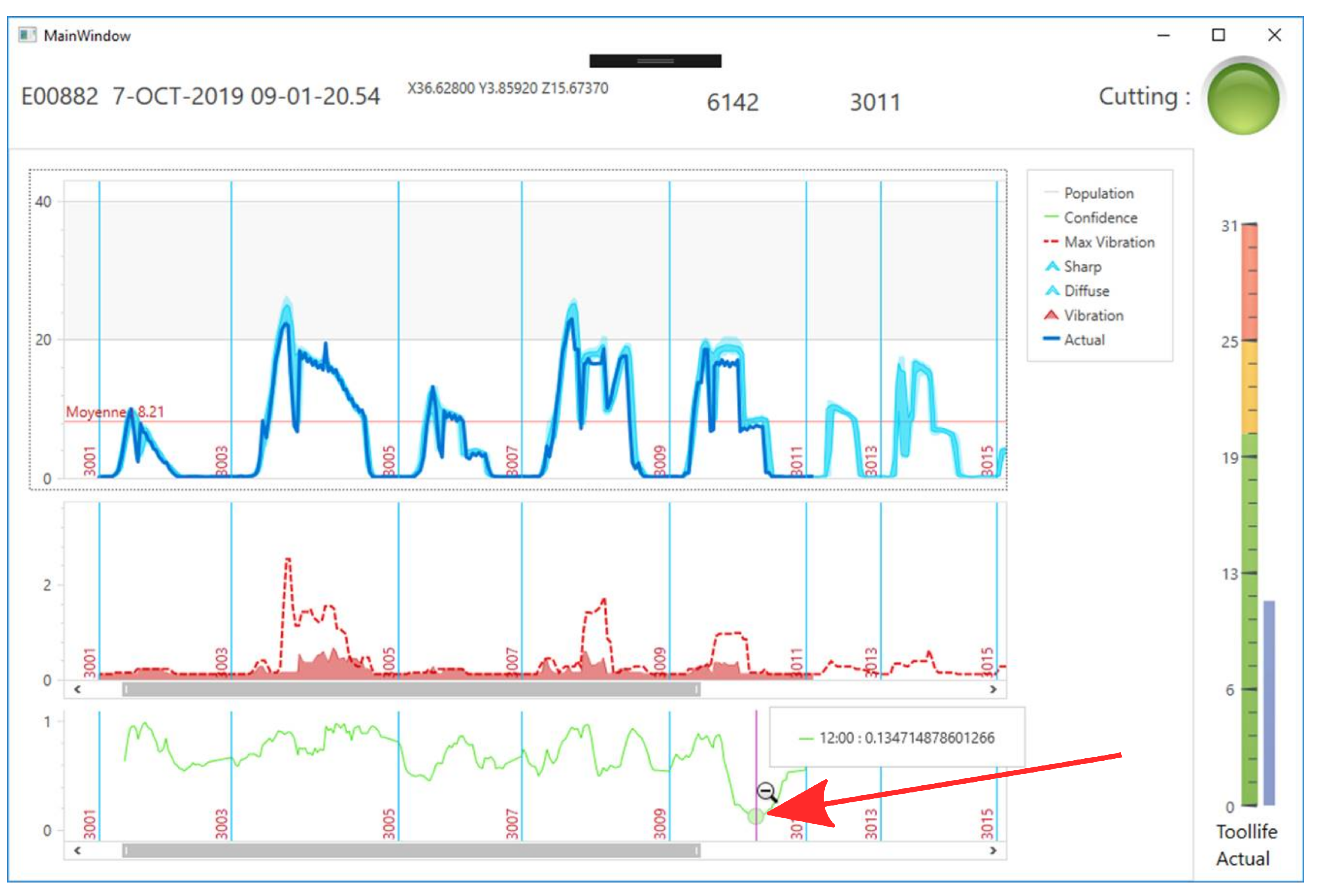
At our industrial partner we tested the normal behavior estimation to monitor the manufacturing processes of titanium parts of their production line. Figure A1 shows the graphical interface of the program developed for this purpose. The program monitors the spindle load (blue line) as well as the maximum vibration of the machine (red dotted line). The pale blue region of the upper part of Figure A1 is the region considered as normal behavior while the blue line is the live spindle load of the current process. The red region in the middle part of Figure A1 represents the maximum vibration. The green line, at the bottom part of Figure A1 is a statistical z-test. The z-test was computed as a running test over past and current data. The test was used to determine if the current spindle; the blue line is part of the normal distribution (pale blue region). Since the z-test keeps information from previously received data, it keeps a score near 1 as long as most of the data are inside the blue region. One point out of the zone will not make it decrease instantly, but if multiple points are outside the normal behavior region, then it will decrease. This can be seen between sub-programs 3009 and 3011 in Figure A1. The spindle load fell below the pale blue region and the green line started to decrease. This is an indicator that the process might be faulty and that the part needs to be inspected. The goal of such a program is to automatically detect whether the part production process is going as intended.
Figure A1.
Testing the normal behavior monitoring of program behavior.

References
- Mohanraj, T.; Shankar, S.; Rajasekar, R.; Sakthivel, N.; Pramanik, A. Tool condition monitoring techniques in milling process—A review. J. Mater. Res. Technol. 2020, 9, 1032–1042. [Google Scholar] [CrossRef]
- Baur, M.; Albertelli, P.; Monno, M. A review of prognostics and health management of machine tools. Int. J. Adv. Manuf. Technol. 2020, 107, 2843–2863. [Google Scholar] [CrossRef]
- Chen, H.; Huang, W.; Huang, J.; Cao, C.; Yang, L.; He, Y.; Zeng, L. Multi-fault Condition Monitoring of Slurry Pump with Principle Component Analysis and Sequential Hypothesis Test. Int. J. Pattern Recognit. Artif. Intell. 2019, 34, 2059019. [Google Scholar] [CrossRef]
- Kundu, P.; Darpe, A.K.; Kulkarni, M.S. A review on diagnostic and prognostic approaches for gears. Struct. Health Monit. 2020. [Google Scholar] [CrossRef]
- Lo, C.C.; Lee, C.H.; Huang, W.C. Prognosis of bearing and gear wears using convolutional neural network with hybrid loss function. Sensors 2020, 20, 3539. [Google Scholar] [CrossRef] [PubMed]
- Álvaro, H.H.; Pliego, M.A.; García Márquez, F.P. Photovoltaic plant condition monitoring using thermal images analysis by convolutional neural network-based structure. Renew. Energy 2020, 153, 334–348. [Google Scholar] [CrossRef] [Green Version]
- Salimiasl, A.; Özdemir, A. Analyzing the performance of artificial neural network (ANN)-, fuzzy logic (FL)-, and least square (LS)-based models for online tool condition monitoring. Int. J. Adv. Manuf. Technol. 2016, 87, 1145–1158. [Google Scholar] [CrossRef]
- Dalenogare, L.S.; Benitez, G.B.; Ayala, N.F.; Frank, A.G. The expected contribution of Industry 4.0 technologies for industrial performance. Int. J. Prod. Econ. 2018, 204, 383–394. [Google Scholar] [CrossRef]
- Yaqoob, I.; Ahmed, E.; Hashem, I.A.T.; Ahmed, A.I.A.; Gani, A.; Imran, M.; Guizani, M. Internet of Things Architecture: Recent Advances, Taxonomy, Requirements, and Open Challenges. IEEE Wirel. Commun. 2017, 24, 10–16. [Google Scholar] [CrossRef]
- Bag, S.; Wood, L.C.; Xu, L.; Dhamija, P.; Kayikci, Y. Big data analytics as an operational excellence approach to enhance sustainable supply chain performance. Resour. Conserv. Recycl. 2020, 153, 104559. [Google Scholar] [CrossRef]
- Yu, Y.; Hu, T.; Zeng, C.; Bian, Z.; Meng, L. Element analysis and wear longevity calculation of an O-ring in the actuator cylinder of a certain aircraft landing gear. In Proceedings of the 2017 Prognostics and System Health Management Conference (PHM-Harbin), Harbin, China, 9–12 July 2017; pp. 1–4. [Google Scholar] [CrossRef]
- Schlechtingen, M.; Santos, I.F.; Achiche, S. Wind turbine condition monitoring based on {SCADA} data using normal behavior models. Part 1: System description. Appl. Soft Comput. 2013, 13, 259–270. [Google Scholar] [CrossRef]
- Zhang, W.; Li, C.; Peng, G.; Chen, Y.; Zhang, Z. A deep convolutional neural network with new training methods for bearing fault diagnosis under noisy environment and different working load. Mech. Syst. Signal Process. 2018, 100, 439–453. [Google Scholar] [CrossRef]
- Imad, M.; Hosseini, A.; Kishawy, H.A. Optimization Methodologies in Intelligent Machining Systems—A Review. IFAC-PapersOnLine 2019, 52, 282–287. [Google Scholar] [CrossRef]
- Hopkins, C.; Hosseini, A. A Review of Developments in the Fields of the Design of Smart Cutting Tools, Wear Monitoring, and Sensor Innovation. IFAC-PapersOnLine 2019, 52, 352–357. [Google Scholar] [CrossRef]
- Lu, Y.; Huang, H.; Liu, C.; Xu, X. Standards for Smart Manufacturing: A review. In Proceedings of the 2019 IEEE 15th International Conference on Automation Science and Engineering (CASE), Vancouver, BC, Canada, 22–26 August 2019; pp. 73–78. [Google Scholar] [CrossRef]
- Caggiano, A. Cloud-based manufacturing process monitoring for smart diagnosis services. Int. J. Comput. Integr. Manuf. 2018, 31, 612–623. [Google Scholar] [CrossRef]
- Siddhartha, B.; Chavan, A.P.; Subramanya, K. IoT Enabled Real-Time Availability and Condition Monitoring of CNC Machines. In Proceedings of the 2020 IEEE International Conference on Internet of Things and Intelligence System (IoTaIS), Bali, Indonesia, 27–28 January 2021; pp. 78–84. [Google Scholar]
- Dehnad, K. Density Estimation for Statistics and Data Analysis. Technometrics 1987, 29, 495. [Google Scholar] [CrossRef]
- Jin, X.; Sun, Y.; Que, Z.; Wang, Y.; Chow, T.W.S. Anomaly Detection and Fault Prognosis for Bearings. IEEE Trans. Instrum. Meas. 2016, 65, 2046–2054. [Google Scholar] [CrossRef]
- Rafiee, J.; Arvani, F.; Harifi, A.; Sadeghi, M.H. Intelligent condition monitoring of a gearbox using artificial neural network. Mech. Syst. Signal Process. 2007, 21, 1746–1754. [Google Scholar] [CrossRef]
- Bhuiyan, M.; Choudhury, I.; Dahari, M.; Nukman, Y.; Dawal, S. Application of acoustic emission sensor to investigate the frequency of tool wear and plastic deformation in tool condition monitoring. Measurement 2016, 92, 208–217. [Google Scholar] [CrossRef]
- Rivero, A.; López de Lacalle, L.; Penalva, M.L. Tool wear detection in dry high-speed milling based upon the analysis of machine internal signals. Mechatronics 2008, 18, 627–633. [Google Scholar] [CrossRef]
- Zhang, F.; Liu, Y.; Chen, C.; Li, Y.F.; Huang, H.Z. Fault diagnosis of rotating machinery based on kernel density estimation and Kullback-Leibler divergence. J. Mech. Sci. Technol. 2014, 28, 4441–4454. [Google Scholar] [CrossRef]
- Lee, W.J.; Mendis, G.P.; Triebe, M.J.; Sutherland, J.W. Monitoring of a machining process using kernel principal component analysis and kernel density estimation. J. Intell. Manuf. 2020, 31, 1175–1189. [Google Scholar] [CrossRef]
- Agogino, A.; Goebel, K. Milling Data Set. NASA Ames Prognostics Data Repository, BEST lab, UC Berkeley, Mofett Field, CA. 2007. Available online: https://ti.arc.nasa.gov/tech/dash/groups/pcoe/prognostic-data-repository (accessed on 23 March 2021).
- Chen, Y.C. A Tutorial on Kernel Density Estimation and Recent Advances. arXiv 2017, arXiv:1704.03924. [Google Scholar] [CrossRef]
- Usop, Z.; Sarhan, A.A.D.; Mardi, N.A.; Wahab, M.N.A. Measuring of positioning, circularity and static errors of a CNC Vertical Machining Centre for validating the machining accuracy. Measurement 2015, 61, 39–50. [Google Scholar] [CrossRef]
- Sheather, S.J.; Jones, M.C. A Reliable Data-Based Bandwidth Selection Method for Kernel Density Estimation. J. R. Stat. Soc. Ser. B 1991, 53, 683–690. [Google Scholar] [CrossRef]
Figure 1.
Diagram of data relationship at our industrial partner.

Figure 2.
High level diagram of a machining program for complex parts manufacturing used by our industrial partner.
Figure 2.
High level diagram of a machining program for complex parts manufacturing used by our industrial partner.

Figure 3.
Spindle load through time compared with historical data.

Figure 4.
Raw data for the program 1543 and tool 6040 on the T5-1 machine.

Figure 5.
Raw data for the program 1543 and tool 6040 on the T5-1 machine for run 127.

Figure 6.
Spindle load probability density estimation on time bins of 3 s for program 1543, tool 6040 and machine T5-1 represented as a heat map.
Figure 6.
Spindle load probability density estimation on time bins of 3 s for program 1543, tool 6040 and machine T5-1 represented as a heat map.

Figure 7.
Program 1543 tool 6040 on machine T5-1 normal behavior extraction.

Figure 8.
Normal behavior without run 237 and 241 and raw data on top.


Table 1.
Parameters extracted from the Computer Numerical Control (CNC) machine tools’ controller.
| Data | Units |
|---|---|
| Date | Y/M/D H:m:s:mill |
| Motor Coil Temperature | C |
| Front Bearing Temperature | C |
| Rear Bearing Temperature | C |
| Actual Spindle Speed | RPM |
| Command Spindle Speed | RPM |
| Spindle Override | % |
| Spindle Direction | CW, CCW, STOP, ORIENTATION |
| Instructed Feed | [mm/min], [in./min] |
| Feed Override | % |
| Cutting Signal | ON / OFF |
| Jog Override | % |
| Rapid Override | % |
| Feed Signal axis | % |
| Relative Position | [mm], [in.], [] |
| Absolute Position | [mm], [in.], [] |
| Machine Position | [mm], [in.], [] |
| Distance to go | [mm], [in.], [] |
| Feed Load | % |
| NC MODE | MEMORY, MIDI, REMOTE |
| Spindle FTN | # |
| Spindle ITN | # |
| Main Program | # |
| Exec Program | # |
| Seq Number | # |
| Execution Block | G-Code |
| Block Counter | # |
| Vibration (x, y, z) | g |
| Spindle Load | % |
Table 2.
Average scores for each run of the machining program.
| Run | Score (%) |
|---|---|
| 69 | 68.37 |
| 73 | 74.47 |
| 89 | 51.89 |
| 93 | 73.47 |
| 127 | 63.26 |
| 131 | 59.03 |
| 135 | 80.28 |
| 186 | 77.47 |
| 190 | 80.13 |
| 194 | 56.44 |
| 233 | 80.00 |
| 237 | 47.52 |
| 241 | 45.34 |
| 320 | 63.22 |
| 324 | 63.93 |
| 328 | 73.30 |
| 354 | 68.85 |
| 356 | 77.91 |
Publisher’s Note: MDPI stays neutral with regard to jurisdictional claims in published maps and institutional affiliations. |
© 2021 by the authors. Licensee MDPI, Basel, Switzerland. This article is an open access article distributed under the terms and conditions of the Creative Commons Attribution (CC BY) license (http://creativecommons.org/licenses/by/4.0/).
Share and Cite
MDPI and ACS Style
Bernard, G.; Achiche, S.; Girard, S.; Mayer, R. Condition Monitoring of Manufacturing Processes under Low Sampling Rate. J. Manuf. Mater. Process. 2021, 5, 26. https://0-doi-org.brum.beds.ac.uk/10.3390/jmmp5010026
AMA Style
Bernard G, Achiche S, Girard S, Mayer R. Condition Monitoring of Manufacturing Processes under Low Sampling Rate. Journal of Manufacturing and Materials Processing. 2021; 5(1):26. https://0-doi-org.brum.beds.ac.uk/10.3390/jmmp5010026
Chicago/Turabian StyleBernard, Gabriel, Sofiane Achiche, Sébastien Girard, and René Mayer. 2021. "Condition Monitoring of Manufacturing Processes under Low Sampling Rate" Journal of Manufacturing and Materials Processing 5, no. 1: 26. https://0-doi-org.brum.beds.ac.uk/10.3390/jmmp5010026