
Spatial Distribution Analyses of Axially Long Plasmas under a Multi-Cusp Magnetic Field Using a Kinetic Particle Simulation Code KEIO-MARC
 , and
, and
Abstract
:1. Introduction
2. Simulation Model
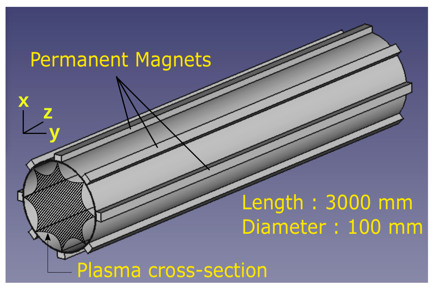
2.1. Plasma Source
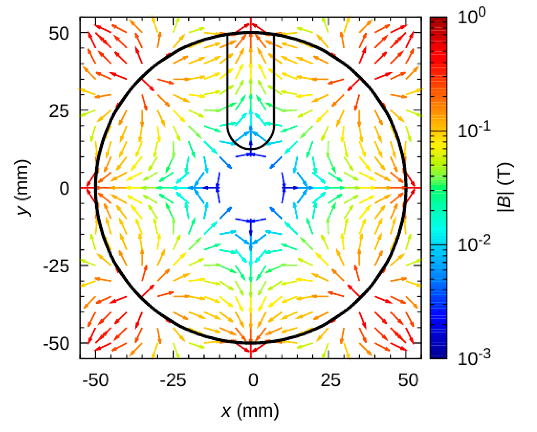
2.2. Calculation of Multi-Cusp Magnetic Field
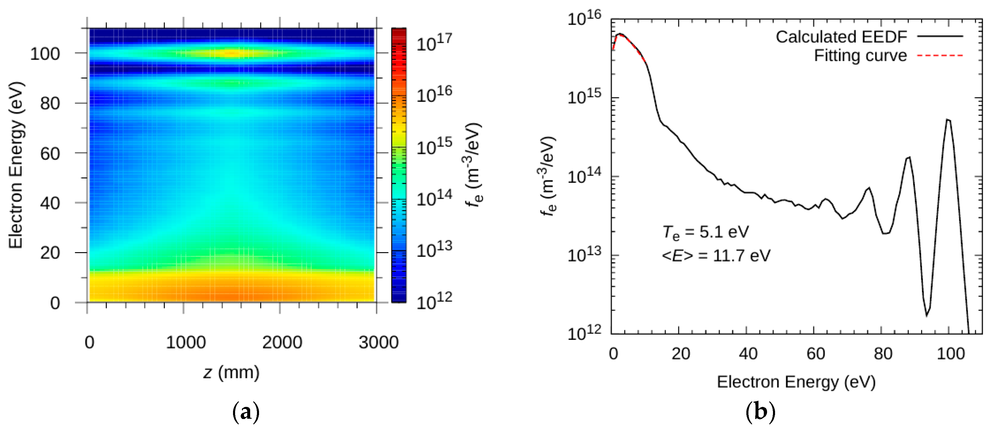
2.3. Calculation of Electron Energy Distribution Function
3. Simulation Results
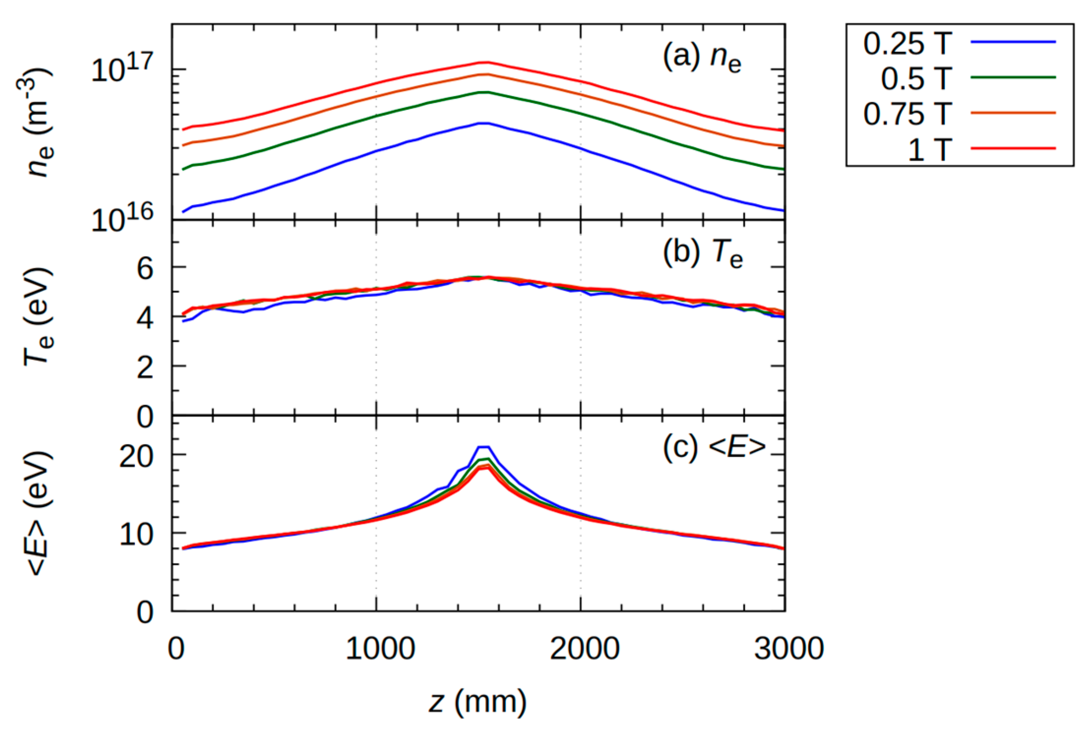
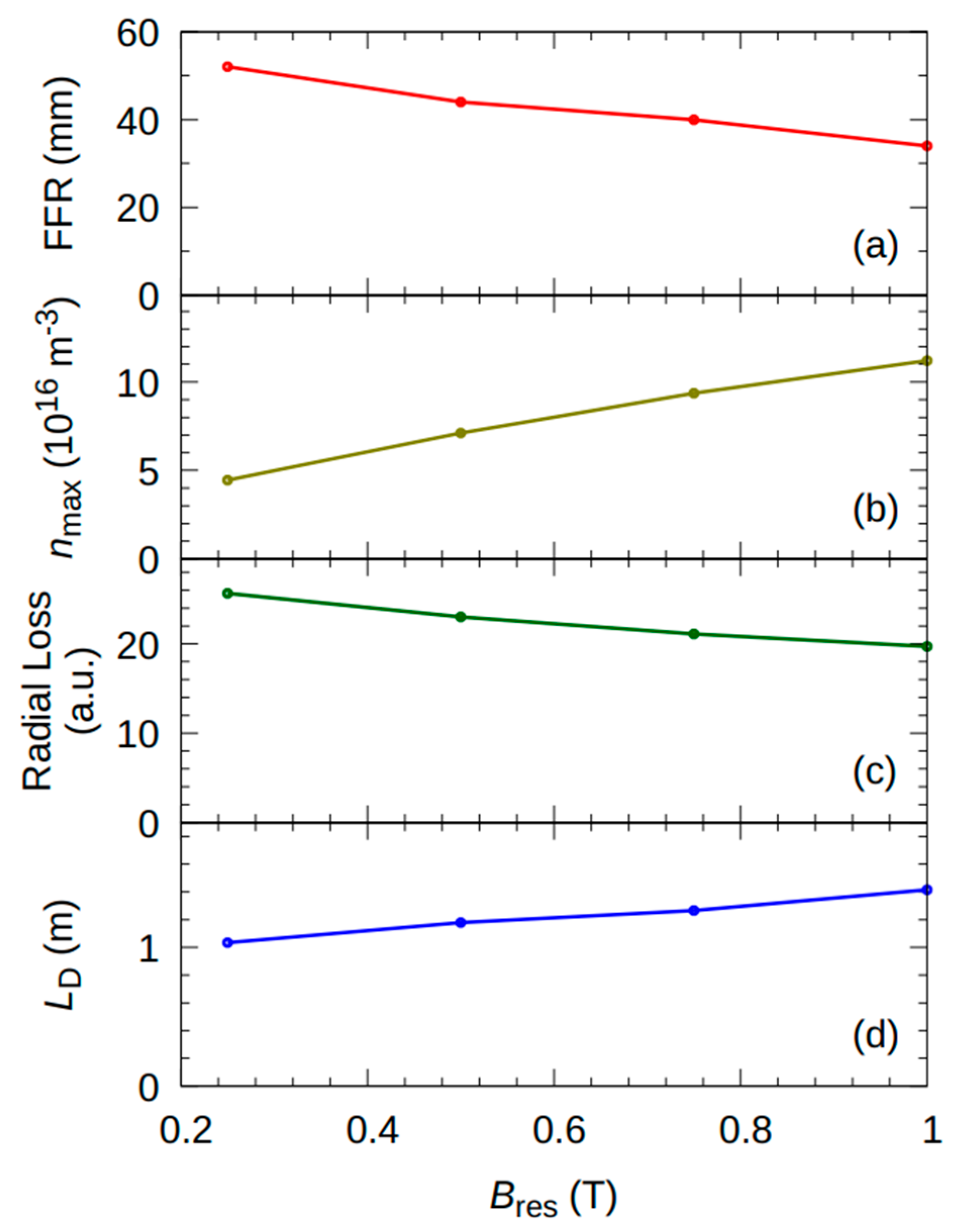
3.1. Effect of the Radial Magnetic Flux Density Bres on Plasma Axial Distribution
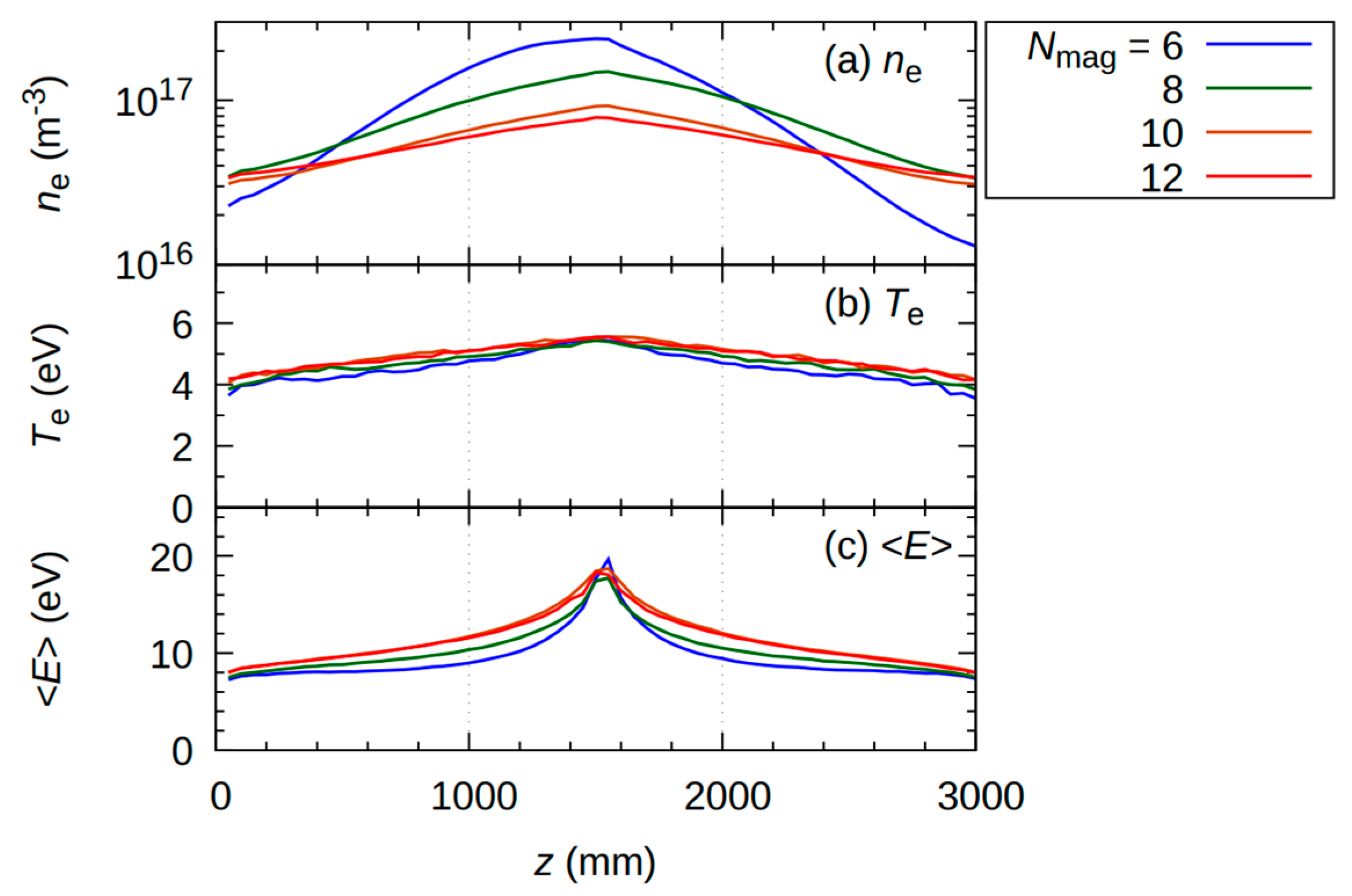
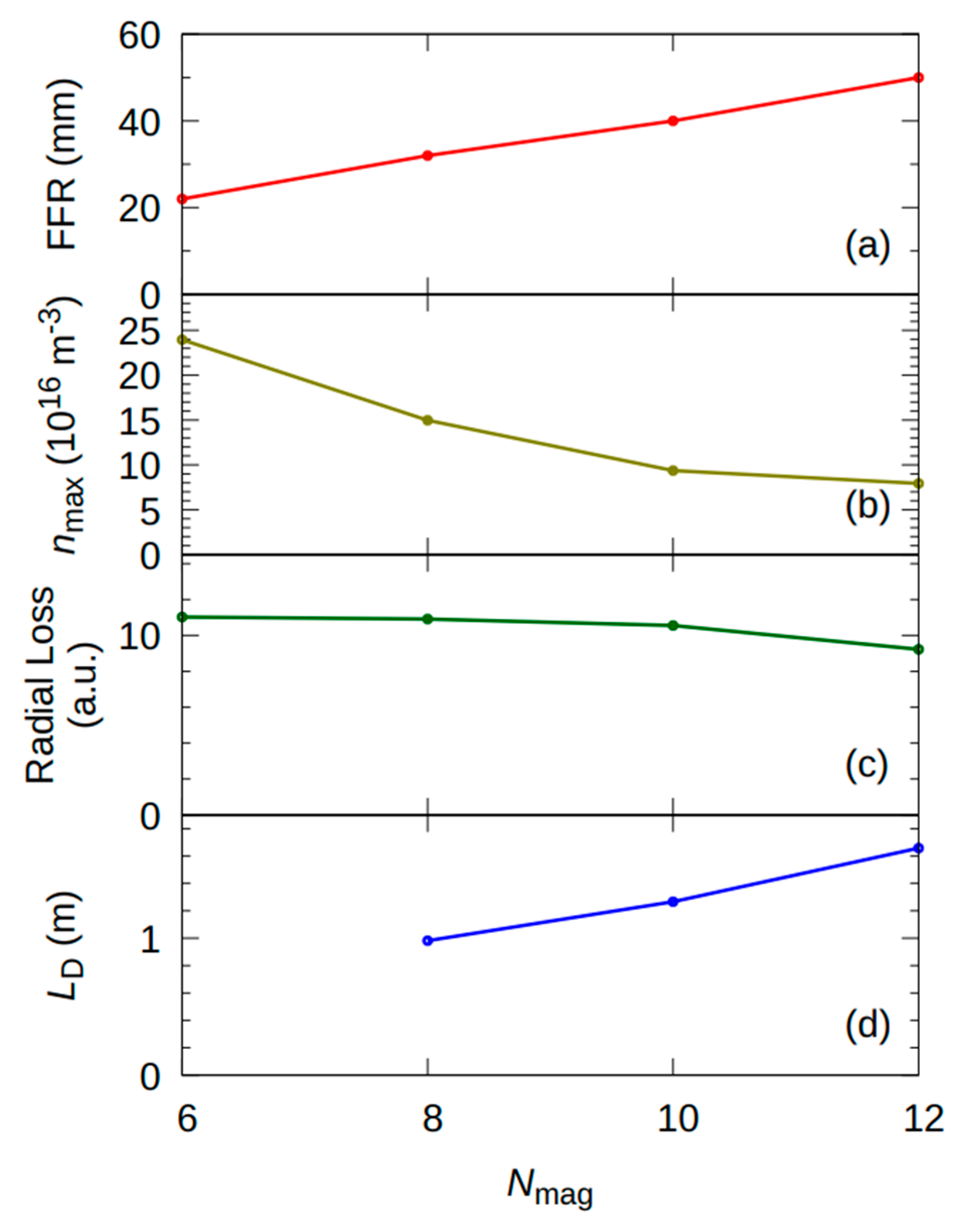
3.2. Effect of the Number of Magnets Nmag on Plasma Axial Distribution
3.3. Effect of Increasing the Number of Filaments on the Axial Plasma Distribution
4. Conclusions
Author Contributions
Funding
Institutional Review Board Statement
Informed Consent Statement
Data Availability Statement
Conflicts of Interest
References
- Takeiri, Y.; Ando, A.; Keneko, O.; Oka, Y.; Akiyama, R.; Asano, R.; Kawamoto, T.; Kuroda, T.; Tanaka, M.; Kawakami, H. Development of an intense negative hydrogen ion source with an external magnetic filter. Rev. Sci. Instrum. 1995, 66, 2541–2546. [Google Scholar] [CrossRef]
- Takeiri, Y. Negative ion source development for fusion application. Rev. Sci. Instrum. 2010, 81, 02B114. [Google Scholar] [CrossRef]
- Jayamanna, K.; Ames, F.; Bylinskii, I.; Lovera, M.; Minato, B. A 60 mA DC H− multi cusp ion source developed at TRIUMF. Nucl. Instrum. Methods Phys. Res. A 2018, 895, 150–157. [Google Scholar] [CrossRef]
- Jia, X.; Zhang, T.; Zheng, X.; Qin, J. Development of a compact filament-discharge multi-cusp H− ion source. Rev. Sci. Instrum. 2013, 83, 02A730. [Google Scholar] [CrossRef]
- Kim, J.H. Numerical simulation of a multi-cusp ion source for high current H− cyclotron at RISP. Phys. Procedia 2015, 66, 498–505. [Google Scholar] [CrossRef]
- Ohara, Y.; Akiba, M.; Horiike, H.; Inami, H.; Okumura, Y.; Tanaka, S. 3D computer simulation of the primary electron orbits in a magnetic multipole plasma source. J. Appl. Phys. 1987, 61, 1323–1328. [Google Scholar] [CrossRef]
- Hoseinzade, M.; Nijatie, A. Development of H- multicusp ion source. Radiat. Detect. Technol. Meth. 2018, 2, 27. [Google Scholar] [CrossRef]
- Wicker, T.E.; Mantei, T.D. Plasma etching in a multipolar discharge. J. Appl. Phys. 1985, 57, 1638. [Google Scholar] [CrossRef]
- Cooper, C.M.; Weisberg, D.B.; Khalzov, I.; Milhone, J.; Flanagan, K.; Peterson, E.; Wahl, C.; Forest, C.B. Direct measurement of the plasma loss width in an optimized, high ionization fraction, magnetic multi-dipole ring cusp. Phys. Plasmas 2016, 23, 102505. [Google Scholar] [CrossRef]
- Jiang, Y.; Fubiani, G.; Garrigues, L.; Boeuf, J.P. Magnetic cusp confinement in low-β plasmas revisited. Phys. Plasmas 2020, 27, 113506. [Google Scholar] [CrossRef]
- Patel, A.D.; Sharma, M.; Ramasubramanian, N.; Ganesh, R.; Chattopadhyay, P.K. A new multi-line cusp magnetic field plasma device (MPD) with variable magnetic field. Rev. Sci. Instrum. 2018, 89, 043510. [Google Scholar] [CrossRef]
- Patel, A.D.; Sharma, M.; Ramasubramanian, N.; Ghosh, J.; Chattopadhyay, P.K. Characterization of argon plasma in a variable multi-pole line cusp magnetic field configuration. Phys. Scr. 2020, 95, 035602. [Google Scholar] [CrossRef]
- Leung, K.N.; Samec, T.K.; Lamn, A. Optimization of permanent magnet plasma confinement. Phys. Lett. 1975, 51, 490–492. [Google Scholar] [CrossRef]
- Leung, K.N.; Taylor, G.R.; Barrick, J.M.; Paul, S.L.; Kribel, R.E. Plasma Confinement by permanent magnet boundaries. Phys. Lett. 1976, 57, 145–147. [Google Scholar] [CrossRef]
- Takamura, S. Characteristics if the compact plasma device AIT-PID with multicusp magnetic confinement. IEEJ Trans. 2012, 7 (Suppl. S1), S19–S24. [Google Scholar] [CrossRef]
- Takamura, S.; Ohno, N.; Nishijima, D.; Kajita, S. Formation of Nanostructured Tungsten with Arborescent Shape due to Helium Plasma Irradiation. Plasma Fus. Res. 2006, 1, 051. [Google Scholar] [CrossRef]
- Takamura, S.; Tsujikawa, T.; Tomida, T.; Suzuki, K.; Minagawa, T.; Miyamoto, T.; Ohno, N. Compact Plasma Device for PWI Studies. J. Plasma Fusion Res. Ser. 2010, 9, 441–445. [Google Scholar]
- Takamura, S.; Uesugi, Y. Coupled interactions between tungsten surfaces and transient high-heat-flux deuterium plasmas. Nucl. Fusion 2015, 55, 033003. [Google Scholar] [CrossRef]
- Nishijima, D.; Ye, M.Y.; Ohno, N.; Takamura, S. Formation mechanism of bubbles and holes in tungsten surface with low-energy and high-flux helium plasma irradiation in NAGDIS-II. J. Nucl. Mater. 2004, 329–333, 1029–1033. [Google Scholar] [CrossRef]
- Okamoto, A.; Kado, S.; Kajita, S.; Tanaka, S. Laser Thomson scattering system applicable to low-temperature plasma in the divertor simulator MAP-II. Rev. Sci. Instrum. 2005, 76, 116106. [Google Scholar] [CrossRef]
- Hosseinzadeh, M.; Afarideh, H. Numerical simulation for optimization of multipole permanent magnets of multicusp ion source. Nucl. Instrum. Methods Phys. Res. A 2014, 735, 416–421. [Google Scholar] [CrossRef]
- Hatayama, A.; Nishioka, S.; Nishida, K.; Mattei, S.; Lettry, J.; Miyamoto, K.; Shibata, T.; Onai, M.; Abe, S.; Fujita, S.; et al. Present status of numerical modeling of hydrogen negative ion source plasmas and its comparison with experiments: Japanese activities and their collaboration with experimental groups. New J. Phys. 2018, 20, 065001. [Google Scholar] [CrossRef]
- Shibata, T.; Kashiwagi, M.; Inoue, T.; Hatayama, A.; Hanada, M. Numerical study of atomic production rate in hydrogen ion sources with the effect of non-equilibrium electron energy distribution function. J. Appl. Phys. 2013, 114, 143301. [Google Scholar] [CrossRef]
- Hatayama, A.; Shibata, T.; Nishioka, S.; Ohta, M.; Yasumoto, M.; Nishira, K.; Yamamoto, T.; Miyamoto, K.; Fukano, A.; Mizuno, T. Kinetic modeling of particle dynamics in H− negative ion sources. Rev. Sci. Instrum. 2014, 85, 02A510. [Google Scholar] [CrossRef]
- Kato, R.; Hoshino, K.; Nakano, H.; Shibata, T.; Miyamoto, K.; Iwanaka, K.; Hayashi, K.; Hatayama, A. Numerical analysis of isotope effect in NIFS negative ion source. J. Phys. Conf. Ser. 2022, 2244, 012035. [Google Scholar] [CrossRef]
- Onai, M.; Etoh, H.; Aoki, Y.; Shibata, T.; Mattei, S.; Fujita, S.; Hatayama, A.; Lettry, J. Effect of high energy electrons on H− production and destruction in a high current DC negative ion source for cyclotron. Rev. Sci. Instrum. 2016, 87, 02B127. [Google Scholar] [CrossRef] [PubMed]
- Etoh, H.; Onai, M.; Aoki, Y.; Mitsubori, H.; Arakawa, Y.; Sakuraba, J.; Kato, T.; Mitsumoto, T.; Hiasa, T.; Yajima, S.; et al. High current DC negative ion source for cyclotron. Rev. Sci. Instrum. 2016, 87, 02B135. [Google Scholar] [CrossRef]
- Yamada, S.; Kitami, H.; Nomura, S.; Aoki, Y.; Hoshino, K.; Hatayama, A. Numerical Simulation for Enhancement of H− Production in the DC Arc-Discharge Hydrogen Negative Ion Source for Medical Use. Plasma Fus. Res. 2019, 14, 3401160. [Google Scholar] [CrossRef]
- Yoshida, M.; Hanada, M.; Kojima, A.; Kashiwagi, M.; Grisham, R.L.; Hatayama, A.; Shibata, T.; Yamamoto, T.; Akino, N.; Endo, Y.; et al. 22 A beam production of the uniform negative ions in the JT-60 negative ion source. Fusion Eng. Des. 2015, 96–97, 616–619. [Google Scholar] [CrossRef]
- Takado, N.; Tobari, H.; Inoue, T.; Hanatani, J.; Hatayama, A.; Hanada, M.; Kashiwagi, M.; Sakamoto, K. Numerical analysis of the production profile of H0 atoms and subsequent H− ions in large negative ion sources. J. Appl. Phys. 2008, 103, 053302. [Google Scholar] [CrossRef]
- Yoon, J.; Song, M.; Han, J.; Hwang, S.H.; Chang, W.; Lee, B.; Itikawa, Y. Cross sections for electron collisions with hydrogen molecules. J. Phys. Chem. Ref. Data 2008, 37, 913–931. [Google Scholar] [CrossRef]


| Particle | Temperature (K) | Density (m−3) |
|---|---|---|
| H2 | 500 | 2.9 × 10¹⁹ |
| H | 1000 | 2.9 × 10¹⁷ |
| H+ | 5800 | 1.0 × 10¹⁷ |
| H2+ | 1000 | 1.0 × 10¹⁵ |
| H3+ | 1000 | 1.0 × 10¹⁵ |
Disclaimer/Publisher’s Note: The statements, opinions and data contained in all publications are solely those of the individual author(s) and contributor(s) and not of MDPI and/or the editor(s). MDPI and/or the editor(s) disclaim responsibility for any injury to people or property resulting from any ideas, methods, instructions or products referred to in the content. |
© 2024 by the authors. Licensee MDPI, Basel, Switzerland. This article is an open access article distributed under the terms and conditions of the Creative Commons Attribution (CC BY) license (https://creativecommons.org/licenses/by/4.0/).
Share and Cite
Nishimura, R.; Seino, T.; Yoshimura, K.; Takahashi, H.; Matsuyama, A.; Hoshino, K.; Oishi, T.; Tobita, K. Spatial Distribution Analyses of Axially Long Plasmas under a Multi-Cusp Magnetic Field Using a Kinetic Particle Simulation Code KEIO-MARC. Plasma 2024, 7, 64-75. https://0-doi-org.brum.beds.ac.uk/10.3390/plasma7010005
Nishimura R, Seino T, Yoshimura K, Takahashi H, Matsuyama A, Hoshino K, Oishi T, Tobita K. Spatial Distribution Analyses of Axially Long Plasmas under a Multi-Cusp Magnetic Field Using a Kinetic Particle Simulation Code KEIO-MARC. Plasma. 2024; 7(1):64-75. https://0-doi-org.brum.beds.ac.uk/10.3390/plasma7010005
Chicago/Turabian StyleNishimura, Ryota, Tomohiro Seino, Keigo Yoshimura, Hiroyuki Takahashi, Akinobu Matsuyama, Kazuo Hoshino, Tetsutarou Oishi, and Kenji Tobita. 2024. "Spatial Distribution Analyses of Axially Long Plasmas under a Multi-Cusp Magnetic Field Using a Kinetic Particle Simulation Code KEIO-MARC" Plasma 7, no. 1: 64-75. https://0-doi-org.brum.beds.ac.uk/10.3390/plasma7010005