Sparse Measurement-Based Coordination of Electric Vehicle Charging Stations to Manage Congestions in Low Voltage Grids


Institute of Energy Systems and Electrical Drives, TU Wien, 1040 Vienna, Austria
Smart Cities 2021, 4(1), 17-40; https://0-doi-org.brum.beds.ac.uk/10.3390/smartcities4010002
Submission received: 24 November 2020
/
Revised: 14 December 2020
/
Accepted: 17 December 2020
/
Published: 22 December 2020
(This article belongs to the Special Issue Innovative Energy Systems for Smart Cities)
Abstract
:The increasing use of distributed generation and electric vehicle charging stations provokes violations of the operational limits in low voltage grids. The mitigation of voltage limit violations is addressed by Volt/var control strategies, while thermal overload is avoided by using congestion management. Congestions in low voltage grids can be managed by coordinating the active power contributions of the connected elements. As a prerequisite, the system state must be carefully observed. This study presents and investigates a method for the sparse measurement-based detection of feeder congestions that bypasses the major hurdles of distribution system state estimation. Furthermore, the developed method is used to enable congestion management by the centralized coordination of the distributed electric vehicle charging stations. Different algorithms are presented and tested by conducting load flow simulations on a real urban low voltage grid for several scenarios. Results show that the proposed method reliably detects all congestions, but in some cases, overloads are detected when none are present. A minimal detection accuracy of 73.07% is found across all simulations. The coordination algorithms react to detected congestions by reducing the power consumption of the corresponding charging stations. When properly designed, this strategy avoids congestions reliably but conservatively. Unnecessary reduction of the charging power may occur. In total, the presented solution offers an acceptable performance while requiring low implementation effort; no complex adaptations are required after grid reinforcement and expansion.
1. Introduction
The electricity grid is traditionally divided into the transmission level, which includes the high and very high voltage grids, and the distribution level, which includes the medium and low voltage grids [1]. At each level, the distributed power injections and absorptions may provoke voltage limit violations [2,3] and congestions [3,4,5], i.e., transformer and line overloading. At the transmission level, both types of limit violations are separately addressed by two different operation processes: Volt/var control and congestion management. Volt/var control uses transformers with on-load tap changers (OLTC) and controllable reactive power devices to maintain the grid voltages within the acceptable range [6]. Meanwhile, congestions are managed by manipulating the active power flows, either by rescheduling the injections of power plants or by reallocating the active power flows between different transmission lines [7]. Active power is not used to control the voltage. At the distribution level, the voltage is conventionally controlled by the OLTC of the supplying transformer, and in some cases, supportive capacitor banks are distributed throughout the medium voltage grid [8]. The sufficient dimensioning of distribution grids has obviated the need for congestion management.
Nowadays, the increasing use of distributed energy resources (DER) calls for an adaption of the traditional control strategies. The intensive active power contributions of photovoltaic (PV) systems and electric vehicle charging stations (EVCS) justify the use of Volt/var control and congestion management also at low voltage (LV) level. Besides the use of OLTCs in distribution substations [9] and distributed or concentrated reactive power control [10], the authors of many studies suggest to control the voltage by manipulating the active power flows [11,12,13,14]. This idea mainly arises from the relatively high resistance to inductance (R/X) ratio that prevails in distribution grids. However, active power is the good that is traded between the different grid users. The necessary active power transfer is the raison d’être of the electricity grid, and therefore should not be curtailed unless no other option is available to ensure compliance to the operational limits. Consequently, voltage control is to be accomplished by using OLTC and reactive power control, while congestions are to be managed by manipulating the active power flows. When upgrading distribution grids to increase their hosting capacities for DERs, the first step is to implement an appropriate Volt/var control strategy that reliably maintains the voltage within the acceptable range and allows for the maximal active power transfer. Subsequently, if a thermal overload is expected during peak load conditions, congestion management may be implemented. Emergency-driven demand response is the main instrument of future Smart Grids to mitigate congestions by coordinating the active power contributions of customer plants (CP) [15].
The main resources available for demand response are all categories of storages, i.e., those that do inject the stored power back at the charging point of the grid (Cat. A); those that do not inject the stored power back at the charging point (Cat. B); and those that reduce the electricity consumption at the charging point in the near future (Cat. C) [16]. These resources must be coordinated—in a centralized or decentralized way—to enable the emergency-driven demand response. The decentralized control architecture allows to minimize the data to be exchanged, and to guarantee data privacy by design [17], while it is more robust against communication errors and beneficial to prevent system collapse [18]. But, the centralized system takes less time to create coordination among constituent system parts.
In any case, this coordination requires a controller that observes the system state and specifies set-points for the available control variables so as to prevent limit violations within the observed area. At the transmission level, the system state is observed using state estimation, i.e. an algorithm that converts redundant meter readings and other available information into an estimate of the system state [19,20]. The application of conventional state estimation techniques to distribution grids, especially to LV grids, faces severe challenges due to their high R/X ratio, unbalance, complexity, and the low availability of measurements [21]. Distribution system state estimation (DSSE) algorithms have been developed in the past two decades, but their use is still very limited due to the lack of measurements downstream of the substations, updated and accurate grid models, easy access to data from different parts of the organization and unified data format [20].
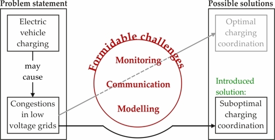
Electric vehicle (EV) batteries are storages of Cat. B that may respond to grid congestions by adapting the active power consumption of the corresponding charging stations [22]. Sophisticated state-of-art coordination schemes consider the electricity price [14,23,24,25], the grid constraints [13,14,23,24,25,26,27], the needs of the EV owners [23,24,25], the grid loss [13,14], and the CO2 emissions [26] to specify the control signals for the distributed EVCSs. These strategies involve high modeling efforts to guarantee compliance to the grid constraints and provoke massive data exchanges, imposing formidable communication challenges.
Within the Austrian flagship project, ‘Power System Cognification (PoSyCo)’ [28] are developed—among many others—algorithms that manage congestions at LV level by the centralized coordination of EVCSs. The focus of this study is set on easy-to-implement but suboptimal solutions that bypass the modeling, monitoring, and communication challenges associated with the state-of-art coordination schemes. New algorithms are developed and simulated on a real urban LV grid that detect congestions based on sparse measurements without requiring state estimation and establishes coordination without requiring network models. The communication requirements are reduced to their minimum.
Section 2 presents the proposed method for the detection of congestions, the algorithms for the coordination of the EVCSs, and the test setup used to simulate the introduced concepts. The simulation results are discussed in detail in Section 3 with a focus on the detection accuracy, LV grid behavior, and battery charging times. The results are discussed in Section 4 and conclusions are drawn in Section 5. Appendix A lists all abbreviations and variables used in the paper.
2. Materials and Methods
Algorithms for the coordination of EVCSs that mitigate enduring overload of LV equipment are presented and simulated in this study. They rely on the sparse measurement-based detection of feeder and distribution transformer (DTR) congestions. To analyze the impact of the algorithms on the behavior of LV grids and on the charging time of the EV batteries, load flow simulations are conducted in a power system model using appropriate software tools. For simplicity, the coordination algorithms and the congestion detection methods are presented for balanced LV grids; their application in unbalanced systems requires minor modifications.
2.1. Sparse Measurement-Based Detection of Feeder Congestions
The detection of feeder congestions is essentially aggravated by the presence of distributed generation. In the past, when the power flows were of unidirectional character, the maximal line segment loading appeared always in the foremost segments, i.e. the line segments connected directly at distribution substation. Nowadays, the distributed injections may provoke the maximum loading somewhere along the feeders, making the detection of congestions exclusively based on distribution substation measurements impracticable.
2.1.1. Mathematical Formulation
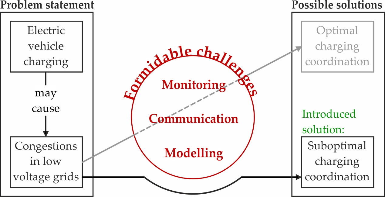
European LV grids are typically of a radial structure, and the CPs are connected somewhere along the feeders [29]. The detailed structure of an LV grid with feeders is schematized in Figure 1a. To each feeder, are connected customer plants that may inject and absorb active and reactive power. Currents with different magnitudes flow through each line segment, provoking the maximum line loading somewhere along the feeders. The calculation of each line segment’s loading in close-to-real-time is possible only when state estimation is applied.
Another option to detect congestions is to estimate the maximum line loading by neglecting the detailed structure of the low voltage feeders. This concept is illustrated in Figure 1b, wherein each feeder is represented by the -symbol, indicating that their detailed structure is not relevant for the calculation procedure. The power balance of each feeder according to Equations (1a) and (1b), in which injections are counted with a positive and absorptions with a negative algebraic sign, builds the basis of the concept.
where , are the active and reactive power flows at feeder beginning (src…source); , are the active and reactive power contributions of CP i; , are the active and reactive power losses occurring in the series impedances of all line segments; and is the reactive power produced by the shunt capacitances of all line segments. In total, the injected active and reactive power always equals the absorbed active and reactive power. To calculate the worst case for the line segment loading, the following assumptions are made:
- The aggregate active () and reactive power injection (), defined in Equations (2a) and (2b), flows through the same line segment of the feeder.
- This line segment is subject to the lowest feeder voltage ().
- This line segment has the lowest thermal limit current () of all line segments.where , , and are determined by Equations (3a)–(3d).
Equations (4a) and (4b) allows for estimating the maximum line segment loading () of the feeder f.
The estimated maximum line segment loading and the measurement of the active power at feeder beginning are used to specify the feeder related congestion flag (), which indicates whether a potential congestion is detected (true) or not (false). It is set to true, when conditions (5a) and (5b) are satisfied, and otherwise to false.
where is the limit of the line segment loading, specified by the grid operator. Condition (5b) roots on the assumption that the feeder is sufficiently dimensioned to cope with the installed PV rating, so that upstream (from feeder end to distribution substation) active power flows do not cause an exceedance of the specified loading limit. This assumption is justified by the following considerations: Due to the spatial proximity of CPs connected to one LV grid, their PV systems always inject simultaneously. The resulting upstream active power flows cannot be reliably reduced by demand response, as the availability of the necessary resources (e.g., EVs connected to EVCSs whose battery is not fully charged) is not guaranteed. The reduction of the PV infeed itself means a waste of renewable energy that should be avoided in any case. Therefore, the only way to allow the full PV injection while avoiding violations of the defined loading limit is to sufficiently dimension the feeder.
2.1.2. Application to Real LV Grid
When applying the algorithm to coordinate the EVCSs connected to a real low voltage grid, several data must be acquired to enable the estimation of the maximum line segment loading. As shown below, this data is derived from the grid data, measurements, and estimations.
| Derived from grid data | |
| Derived from measurements | |
| Estimated |
- Grid Data
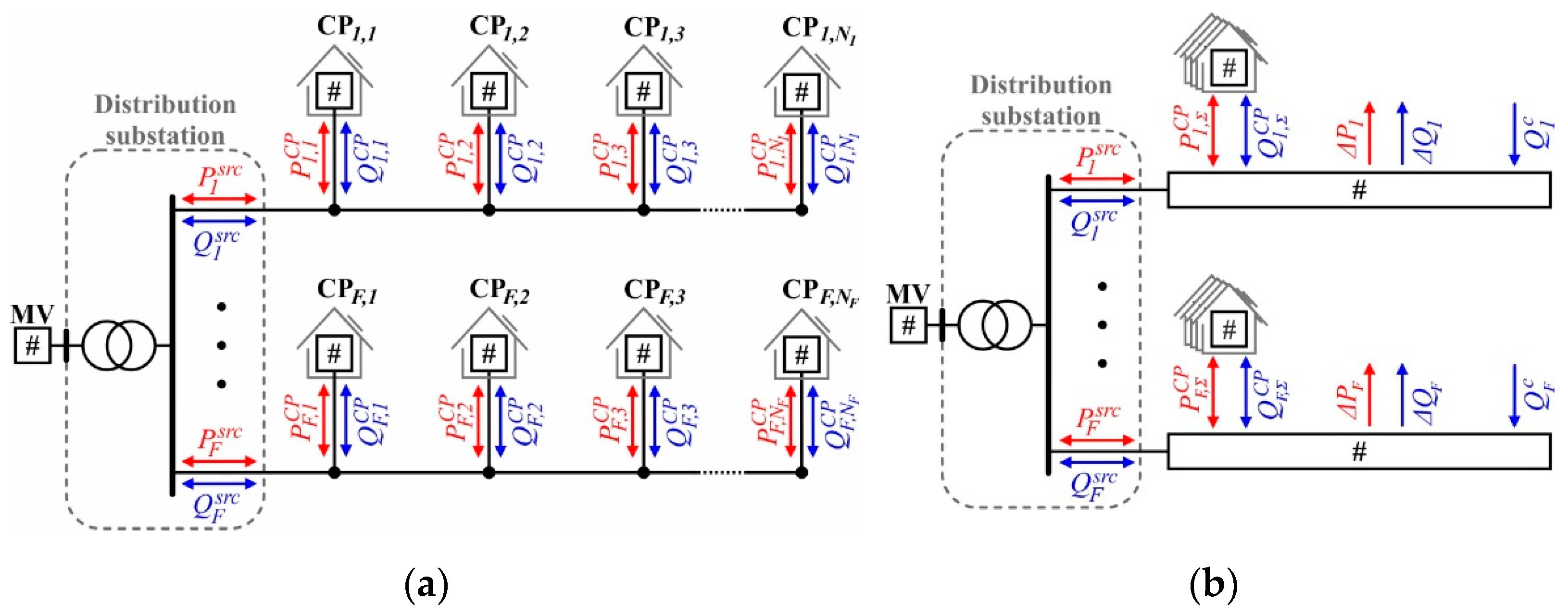
Low voltage feeders typically consist of main and side strands. The side strands usually connect one CP to the main strand, which establishes the connection of all side strands to the distribution substation. The side strands are typically of minor cross-section (e.g., 50 mm²) than the main ones (e.g., 150 mm²), and thus possess lower thermal limit current. While the side strands transmit only the power contributions of the directly connected CP, the main strand is loaded by the power contributions of many CPs, Figure 2.
Consequently, reducing the simultaneity of the CP power contributions by using coordinated electric vehicle charging cannot unload the side strands but only the main ones. Therefore, as specified in Equation (6), the minimal thermal limit current is determined by considering only the line segments of the main strands.
where is the thermal limit current of the line segment , which is part of the main strands of feeder .
- Measurements
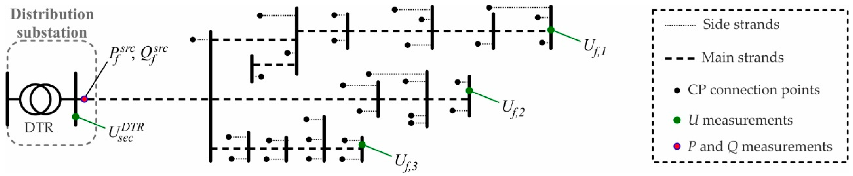
The number of measurement devices should be kept as low as possible to reduce the associated capital expenditures. Figure 3 illustrates the suggested placement of the measurement devices on one representative real low voltage feeder. The active and reactive power flowing into the feeder and the voltage at the secondary bus of the DTR are measured within the distribution substation. In addition, the voltages are measured close to the feeder end. When the feeder is branched and has several ends, more voltage measurements may be necessary.
The active and reactive power injected by the distribution substation is directly derived from the corresponding power measurements using Equations (3a) and (3c). At a low voltage level, the CPs are typically distributed more or less homogeneously along the feeders, and their power contributions lie within the same order of magnitude. All PV systems inject active power simultaneously. As long as no bulk producers (e.g., excessively rated PV system) or consumers (e.g., garage with many EVCSs) are connected in the central portion of the feeder, the voltage usually increases or decreases monotonically along each feeder. In this case, measuring the voltages at the feeder beginning and end is sufficient to capture the minimal voltage value. When bulk producers or consumers are involved, the voltage at their connection points should be measured additionally. As in Equation (7), the minimal feeder voltage is derived by selecting the minimal value of the corresponding measurements.
where is the voltage measurement at feeder ; and is the voltage at the secondary bus bar of the DTR.
- Estimations
The reactive power injected by a shunt capacitance depends on the square of the voltage. Therefore, the amount of reactive power produced by cables and overhead lines at the low voltage level is very small. Hence, it is estimated to be zero, Equation (8).
Each CP may include several devices that contribute active and reactive power, including consuming devices, producers, and storages. On this basis, Equations (9a) and (9b) presents the total active and reactive power contributions of a CP. Its estimation is very difficult and presents the major uncertainty of the proposed method to detect congestions in the LV level.
where , are the aggregate active and reactive power contributions of all consuming devices; , are the aggregate power contributions of all producers; and , are the aggregate power contributions of all storages included in the regarded CP. The customers switch on and off the consuming devices according to their needs, making it almost impossible to forecast the related power contributions for a single CP. Modern consuming devices, such as switch-mode power supply devices without a power factor correction, low power adjustable speed drives, as well as compact fluorescent lamps and light-emitting diodes behave capacitively [30], thus injecting small amounts of reactive power when they are in use. Active power is only absorbed but not injected. Producers connected at the CP level, which are mainly PV systems, may inject active and inject or absorb reactive power. Their active power production depends on the weather conditions, while their reactive power contribution is determined by the applied control strategy, such as constant reactive power, constant power factor, cosφ(P), and Q(U) control [31]. These control strategies are primarily used to mitigate violations of the upper voltage limit in the LV level. Therefore, the constant reactive power, constant power factor, and cosφ(P) controls are set to provoke an inductive behavior of the PV inverter. Q(U) is the only control strategy that leads to capacitive behavior for low feeder voltages. Usually, the customers have to register their PV systems, so that the grid operator knows the installed PV rating, and thus the maximal possible active power injection () of each PV system. When Volt/var control is accomplished by using Q(U) control, the maximal possible reactive power injection () is also known because the grid operator specifies the exact control characteristic. The storage may inject or absorb active power, and in some cases, the corresponding inverters have the capability to contribute reactive power. When no storages of Cat. A are installed (e.g., stationary batteries), the storage component does not inject any active power. Although the authors of some studies suggest operating EVCSs with a non-unity power factor [32,33], their reactive power contribution is usually controlled to be zero. To estimate the maximum power injections of CPs, all consumptions are set to zero and all productions are set to the maximal expected values. Following the above-outlined considerations, and neglecting the reactive power production of modern consuming devices, the maximal CP power injections can be estimated by Equations (10a)–(10c).
Numerous sophisticated strategies exist to estimate the active power contribution of a PV system that use either models of PV systems and forecasts of the meteorological data (mainly irradiance and temperature), or statistical methods and machine learning techniques [34]. In any case, the active power production should rather be over- than underestimated to guarantee the functionality of the proposed congestion detection method. The estimation of the reactive power contribution of Q(U) controlled PV systems is hardly possible without using exact feeder models and state estimation, as it depends on the local feeder voltage. Therefore, although it is very conservative, the use of the maximal possible value according to the specified control characteristic is suggested, Equation (11).
2.2. Detection of DTR Congestions
The loading of the DTR () is calculated based on the measurements in the distribution substation using Equation (12).
where is the rated apparent power of the DTR. When conditions (13a) and (13b) are satisfied, the DTR-related congestion flag () is set to true, and otherwise to false.
where is the limit of the DTR loading, specified by the grid operator.
2.3. Coordination Algorithms
The developed coordination strategy involves two components: the central controller and the distributed EVCSs. It is designed to prevent enduring overload of LV grid equipment based on sparse measurements and a simple communication infrastructure, which allows transmitting one Boolean value from the central controller to all EVCSs connected at the same feeder (unidirectional). State estimation is not required. Both the central controller and the distributed EVCSs are intended to execute algorithms.
Figure 4a shows the algorithm ‘specify permissions’ that is executed by the central controller. It specifies one Boolean control signal per feeder—denoted as feeder permission—that indicates whether the EVCSs connected to the corresponding feeder shall charge with reduced (false) or full power (true). The distribution system operator (DSO) configures the algorithm, i.e. sets the loading limits of the DTR and the line segments, which shall not be exceeded during grid operation. The algorithm is executed periodically, e.g., each 5th minute, to impose low requirements on the associated communication infrastructure. As the first step, the DTR is checked for congestion as described in Section 2.2. When the DTR-related congestion flag is true, all feeder permissions are set to false and are sent out to the EVCSs. Otherwise, each feeder is consecutively checked for congestions according to the procedure described in Section 2.1. If the feeder-related congestion flag is true, the corresponding feeder permission is set to false, and vice versa. When all feeders are checked for congestions, all feeder permissions are sent out to the EVCSs.
Each EVCS periodically (e.g., each second) executes an algorithm to finally set the internal charging power restriction depending on the actual value of the corresponding feeder permission. The execution period must be shorter than that of the central controller and may be set very short as no further communication is required. Three different options for this algorithm are shown in Figure 4b: reduce until next permission, reduce for 30 min, and reduce until the end of charging. The impact of each option on the behavior of the LV grid is analyzed separately in this study.
- Reduce until next permission
The EVCSs update their internal charging power restrictions each time new permissions are received.
- Reduce for 30 min
Option 2 allows charging with maximal power only when the permission is true for at least 30 minutes.
- Reduce until end of charging
This algorithm firstly checks if an EV is currently connected to the EVCS. If this is the case, and a false permission is received, the charging power restriction is reduced to the minimal value until the EV is disconnected.
2.4. Test Setup
To verify their functionality, the algorithms for the sparse measurement-based detection of congestions and the coordination of EVCSs are simulated in a real urban LV grid. The used simulation software and the power system model are described below.
2.4.1. Simulation Software
The developed algorithms are analyzed based on load flow simulations in a combined LV grid and CP model. The power system model is implemented, and the load flow (LF) calculations are conducted in PSS®SINCAL 16.0, while the algorithms are implemented in MATLAB R2019b. Both tools are connected through the COM-interface.
2.4.2. Power System Model
The scope of this study is set on LV and CP levels. Therefore, both levels are included in the used power system model. As the focus is set on the algorithms for congestion management, and Volt/var control has to be implemented prior to congestion management (see Section 1), the Q(U) control strategy is implemented in the PV systems of the CP model. Despite its poor performance compared to more effective control strategies [35,36], it maintains feeder voltages within the acceptable range (±10% around nominal voltage) in the analyzed LV grid due to its relatively short feeders.
- Low voltage grid
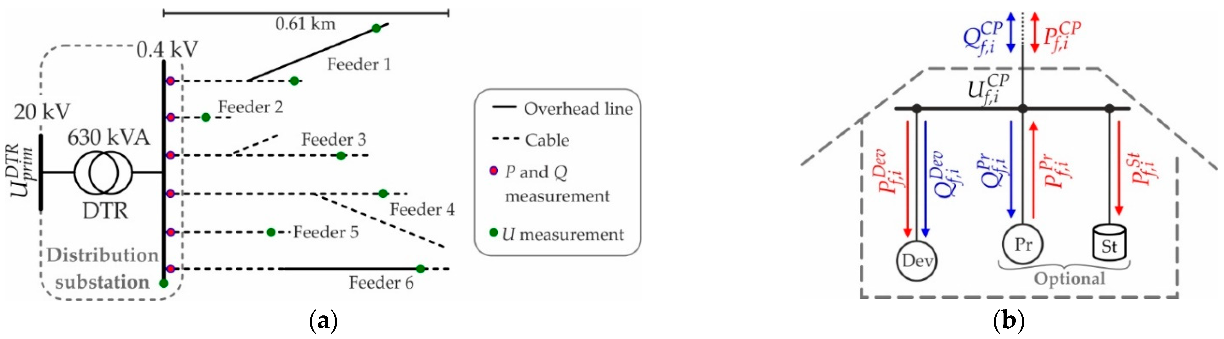
Figure 5a shows the simplified one-line diagram of the LV grid model with the locations of the P-, Q- and U-measurements. Only the main strands are shown, but not the feeder laterals. It represents a real urban grid with a cable share of 81% that connects 91 residential CPs through six feeders. The 20 kV/0.4 kV distribution transformer is rated with 630 kVA and has its tap changer fixed in mid-position. The slack node with the voltage is located at the DTR primary bus bar. In this grid, it is not practicable to install the voltage measurement devices, which are owned and operated by the DSO, at the feeder ends, as CPs are connected at these points. Therefore, they are placed at the backmost distribution cabinet or tower.
Table 1 gives more detailed data for each feeder of the LV grid model.
- Customer plants
Figure 5b shows the structure of the CP model with index i connected at the feeder with index f. It includes three components: the device (Dev), producer (Pr), and storage (St) model, representing the household appliances, the PV system, and the EV battery, respectively. The latter ones are optional as the PV and EVCS penetrations are set to approximately 50%, i.e. 46 CPs include a PV system and an EVCS. Asymmetry is not considered. The Dev-model’s active () and reactive power () contributions depend on the CP supply voltage (), Equations (14a) and (14b). Therein, ZIP-coefficients from [37] are used; and power contributions at nominal voltage are defined by load profiles.
where , are the active and reactive power contributions of the Dev-model for nominal supply voltage; is the normalized supply voltage of the CP; and t is the instant of time. The voltage-independent active power injections of the Pr-models are defined by one common load profile. Meanwhile, their reactive power contributions are determined by the common Q(U)-characteristic suggested as default in [9]. The maximum active () and reactive power () contributions of the Pr-model are set according to Equations (15a) and (15b).
The factor in Equation (15b) is set to derive the maximal reactive power contribution from the maximal active power injection by the power factor of 0.9. The voltage-dependent active power consumption () of the St-model of the CP is determined by Equation (16a); ZIP-coefficients from [38] are used. The corresponding reactive power contribution is set to zero. Equation (16b) is used to calculate the actual state-of-charge () of the EV battery.
where is the active power consumption of the St-model for nominal supply voltage; is the resolution of the load profiles; and is the storage capacity of the EV battery. The battery is charged whenever condition (17) is satisfied.
where is the instant of time in which the corresponding EVCS starts to charge the battery, specified in the scenario definition. When charging, Equations (18a) and (18b) determines the corresponding active power consumption at nominal supply voltage, and otherwise, it is set to zero.
The EVCS-internal charging restriction is set by coordination algorithms described in Section 2.3. When no coordination is applied, all EVCSs charge with 11 kW at nominal supply voltage. The total power injections of the CP are determined by Equations (19a) and (19b).
- Scenario definition
The scenarios, which are the input data of the model, greatly affect the calculated behavior of the LV grid in the presence and in absence of the EVCS coordination. To obtain robust results that allow us to draw general conclusions, three different scenarios are defined. The scenarios differ from each other regarding the instants of time, in which the EVCSs start to charge the corresponding batteries. The slack voltage of and the load profiles shown in Figure 6 are used in all scenarios. The load profiles of the Dev- and Pr-models are created with the tools described in [39,40], respectively, and have a resolution of one minute. For the Dev-model of each CP are used individual profiles; these profiles account for the temporary capacitive behavior, which is provoked by modern consuming devices. Figure 6a shows exemplary profiles that are used for one of the CPs. Due to the spatial proximity of all CPs connected to one LV grid, the same load profile is used for all Pr-models. This profile is characterized by spikes that are provoked by clouds. The proposed concept for the sparse measurement-based detection of congestions requires an estimate of the PV systems’ active power injections (see Equation (10a)). The estimation, which is used in the simulations with EVCS coordination, is shown in grey and dashed lines in Figure 6b.
In each CP, the charging process is started at an individual instant of time. Three different scenarios are considered: ‘Simultaneous charging in the evening’; ‘Simultaneous charging in the morning’; and ‘Charging throughout the day’. In the former two scenarios, the instants of time in which the EVCSs start charging are defined according to a normal distribution with the mean value at 6 p.m. and 9 a.m., respectively, and the standard deviation of 1 h. In the latter scenario, they are defined by a uniform distribution. Initially, the State-of-Charge (SoC) of each EV battery is set to 25%. Each of the three scenarios is simulated for the case without coordination, and for the three different coordination options shown in Figure 4b. Table 2 overviews all conducted simulations.
3. Results
The simulation results are used to analyze the performance of the algorithms in two steps: firstly, the accuracy of the sparse measurement-based detection of feeder congestion is assessed in absence of EVCS coordination. Secondly, the impact of the three different coordination options on the behavior of the LV grid is investigated in detail. The energy losses of the LV grid, i.e. of the DTR and all line segments, and the average charging time per EV ()—calculated according to Equations (20a) and (20b)—are considered in both steps.
where is the active power loss of the DTR; is the active power loss of line segment with index l; is the timespan that the EVCS with index e requires to fully charge the corresponding battery; is the number of EVCSs connected to the LV grid.
3.1. Sparse Measurement-Based Detection of Feeder Congestions
The accuracy of the sparse measurement-based detection of feeder congestions is assessed for each scenario separately. Thereby, the loading limit of each feeder’s line segments is set to 60%, Equation (21).
According to Equation (22), the detection accuracy is calculated for each feeder by dividing the number of instants of time (), in which the feeder-related congestion flag is set correctly, by the total number of simulated instants of time ().
As shown in Equation (10a), the PV injection into each feeder must be estimated to enable the sparse measurement-based detection of congestions. To assess the impact of the estimation accuracy on the detection accuracy, two different cases are considered: estimated and exact values of (see Figure 6b).
3.1.1. Simultaneous Charging in the Evening
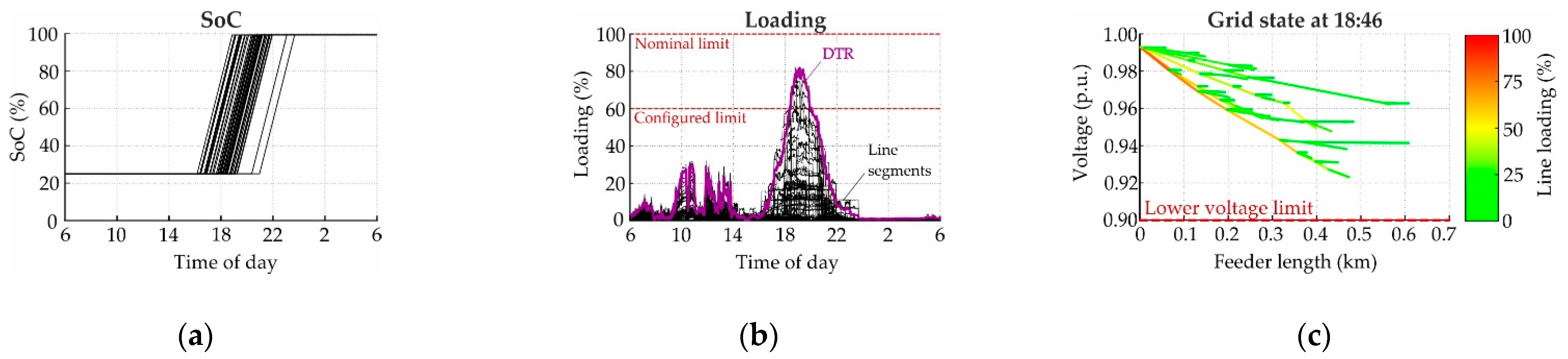
Figure 7 shows the simulation results for the scenario ‘Simultaneous charging in the evening’ without any coordination. The uncoordinated charging with 11 kW per EVCS leads to linear increasing SoCs of the EV batteries between 16:10 and 23:40, Figure 7a. The intensive consumption provokes high loadings of the DTR and all line segments, Figure 7b. They exceed the specified limit between 18:16 and 20:02, while the maximum value appears at 18:46. The resulting grid state at the moment of maximal loading is illustrated in Figure 7c. The voltage profiles of all feeders are plotted on the y-axis, while the line segment loading is presented by color shades from green for 0% loading to red for 100% loading. The diagram shows that no violations of the lower voltage limit and the nominal loading limit appear. The energy losses and the average charging time amount to 56.65 kWh and 161 min, respectively.
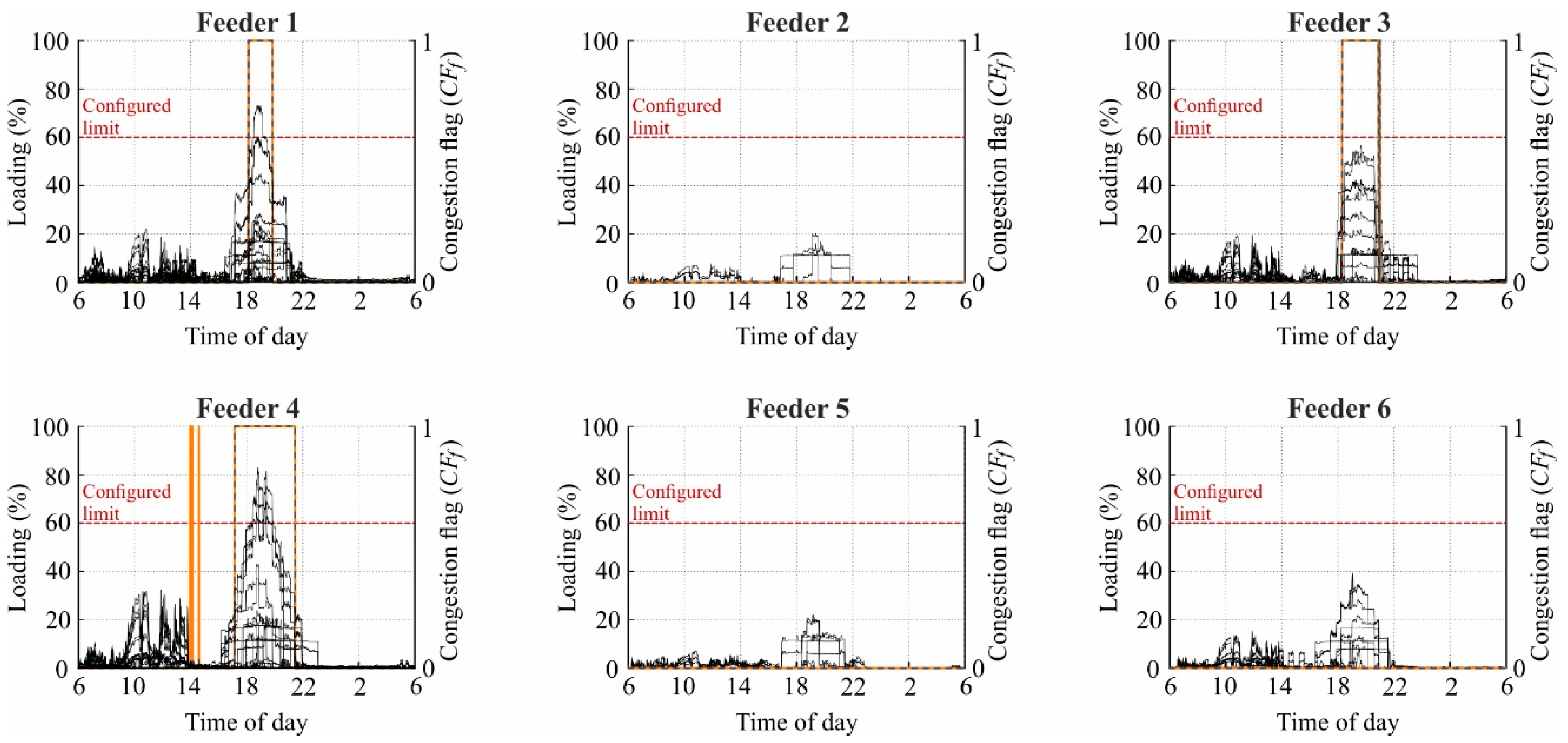
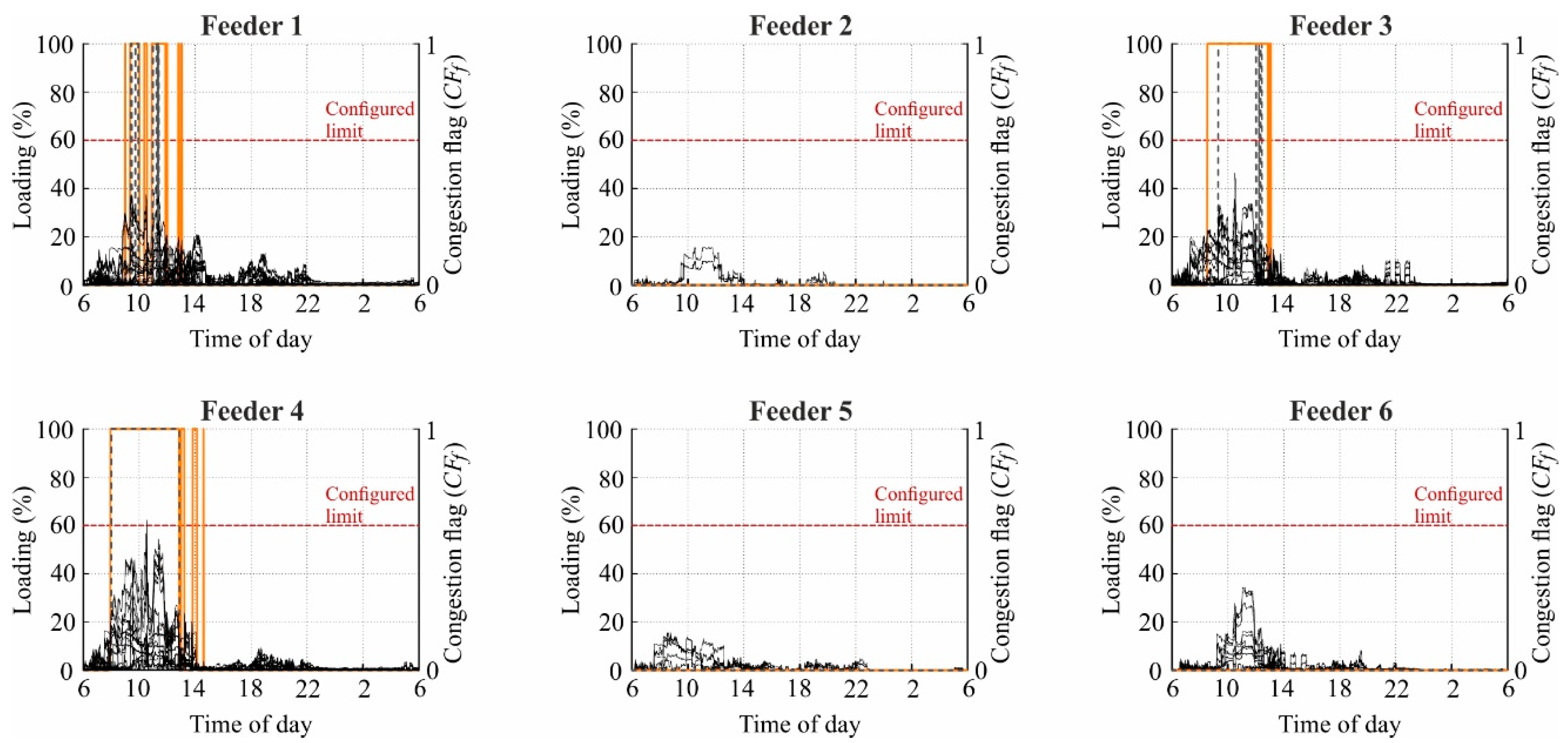
To investigate the behavior of the sparse measurement-based approach to detect feeder congestions, the line segment loadings are shown separately for each feeder in Figure 8. Furthermore, the corresponding congestion flag is shown in orange solid lines for estimated values of , and in dashed grey lines for the exact ones. In both cases, congestions are detected only for feeders 1, 3, and 4. The inaccurate estimation of the PV injection impacts the congestion flag of feeder 4, while no differences occur for the other feeders.
For feeder 1, the congestion flag is true between 18:09 and 19:50, while the configured loading limit is exceeded from 18:26 to 19:20. This corresponds to a detection accuracy of 92.92%. Regarding feeder 3, congestions are detected between 18:18 and 20:53, and at 20:59, although no limit violations appear at all. However, an accuracy of 89.11% is achieved in this case. Feeder 4 exceeds the configured loading limit between 18:16 and 19:55, while congestions are detected from 13:59 to 14:08, at 14:36, and from 17:09 to 21:27, yielding an accuracy of 81.26% when the PV injection is estimated. The exact knowledge of the PV production eliminates the incorrect detections in the early afternoon, improving the detection accuracy to 82.03%. The limit compliance of feeders 2, 5, and 6 is correctly detected with an accuracy of 100%.
3.1.2. Simultaneous Charging in the Morning
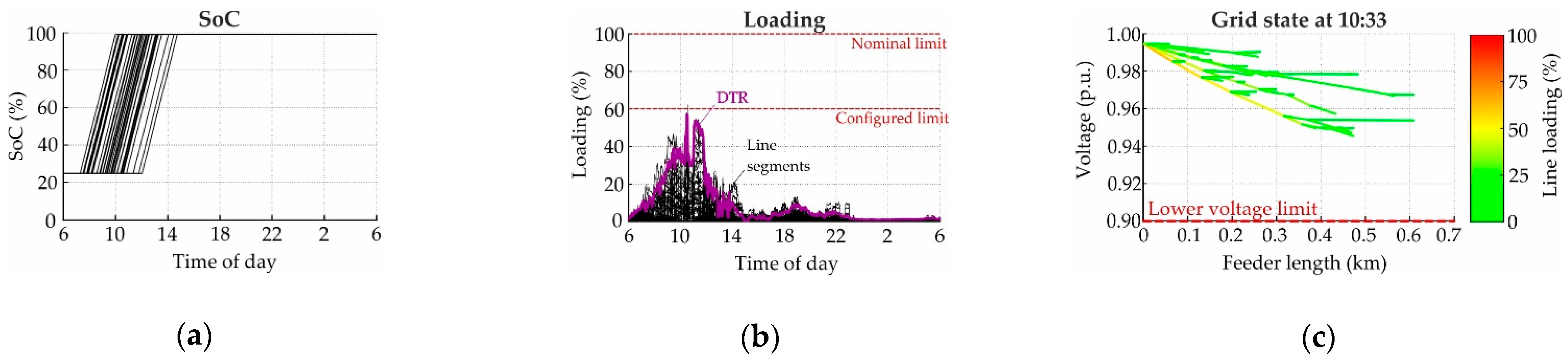
The simulation results for the scenario ‘Simultaneous charging in the morning’ without any coordination are shown in Figure 9. As shown in Figure 9a, the batteries are charged with 11 kW between 7:17 and 14:44, causing one line segment to violate the configured loading limit at 10:33, Figure 9b. The resulting grid state diagram at the moment of maximal loading confirms compliance to the lower voltage and nominal loading limits, Figure 9c. In this scenario, energy losses of 22.28 kWh occur, while the EV batteries are fully charged within 161 min on average.
The line segment loadings and the congestion flag are shown separately for each feeder in Figure 10. As in the above-discussed scenario, congestions are detected for feeders 1, 3, and 4, although violations of the configured loading limit appear only in feeder 4. Meanwhile, the limit compliance of the other feeders is correctly detected with an accuracy of 100%, independently of the used PV estimation accuracy.
When the PV production is estimated, the congestion flag related to feeder 1 alternates between true and false from 9:00 to 13:03, resulting in a detection accuracy of 91.46%. The use of the exact PV injections significantly shortens the interval with alternating congestion flags to less than two hours, i.e. from 9:25 to 11:23. This increases the detection accuracy to 97.57%. Congestion of feeder 3 is wrongly detected between 8:32 and 12:51, at 12:55, and from 13:00 to 13:04, when estimating the PV production. Due to these incorrect detections, the corresponding accuracy amounts to 81.54%. The use of the exact PV injections tightens the timespan of the wrong detection, setting the congestion flag to true between 9:20 and 12:01, at 12:14, and from 12:21 to 12:25, leading to a detection accuracy of 88.27%. Regarding feeder 4 for estimated PV production, the congestion flag is true from 7:57 to 12:51 and subsequently alternates until 14:36, reaching the low detection accuracy value of 77.17%. When the exact PV injections are known and fed into the detection algorithm, the alternating is avoided, and the detection accuracy is increased to 79.67%.
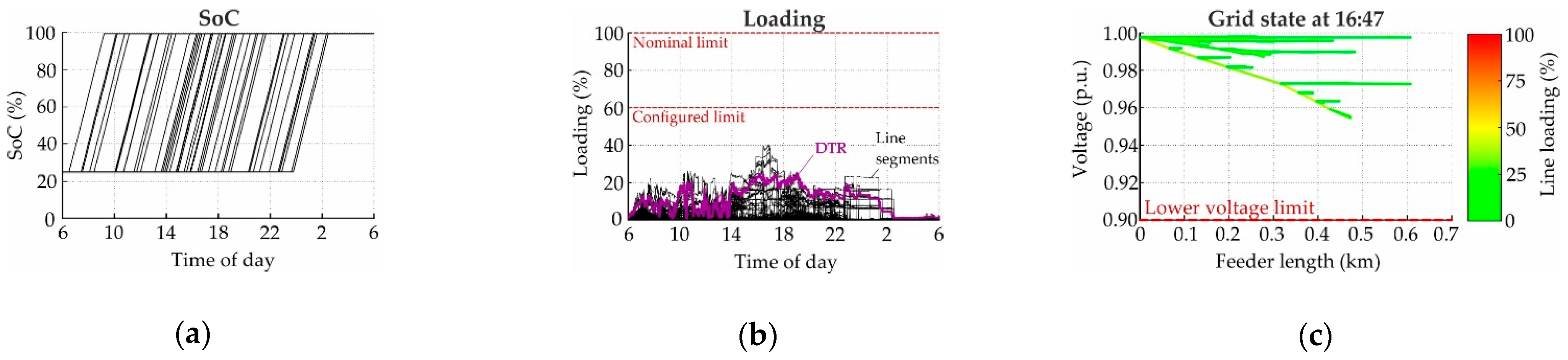
3.1.3. Charging throughout the Day
Figure 11 shows the simulation results for the scenario ‘Charging throughout the day’ without any coordination. The EVCS charge with constant power between 6:30 and 2:29, increasing the SoC of all EV batteries linearly, Figure 11a. Due to the relatively homogenous loading of the grid, the lower voltage limit and the configured and nominal loading limits are satisfied, Figure 11b,c. The maximum line segment loading of 40.26% is reached at 16:47. Here, the energy losses and the average charging time reach 21.31 kWh and 161 min, respectively.
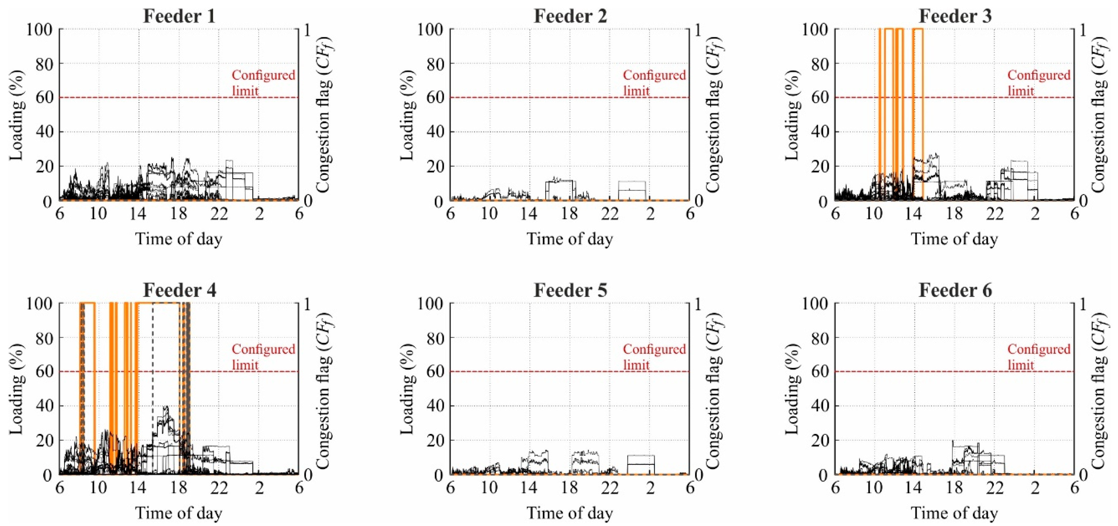
Figure 12 shows the line segment loadings and the feeder-related congestion flag for each feeder separately. Although the configured limit is not violated by any line segment in this scenario, congestions are detected for feeders 3 and 4 when the PV production is estimated. By using the exact PV injections, the incorrect detections related to feeder 3 are completely eliminated. The limit compliance of the other feeders is—for both, estimated and exact PV production—correctly captured by the proposed congestion detection method.
The congestion flags of feeders 3 and 4 alternate many times when the PV production is estimated. For feeder 3, this is the case between 10:29 and 14:49, yielding a detection accuracy of 89.45%. For feeder 4 and estimated PV injections, the alternating takes place from 8:06 to 13:50, and from 18:40 to 19:04. Furthermore, congestion is wrongly detected between 13:50 and 18:40, yielding an accuracy of 73.07%. The use of the exact PV production improves the detection accuracy to 87.30%, as the alternating in the early afternoon is avoided, and the timespan of sustained congestion detection is significantly shortened.
3.2. Coordination Algorithms
The impact of the coordination algorithms described in Section 3 on the behavior of the LV grid and the SoC of the EV batteries is investigated for each scenario separately. The central controller specifies and sends out permissions each 5th minute, while the load flow simulations are conducted in one-minute time steps. For the sparse measurement-based detection of congestions, which builds the basis of the coordination algorithms, the estimated PV production according to Figure 6b is used. The loading limits of the DTR and the feeders are configured to 60%, Equations (23a) and (23b).
3.2.1. Simultaneous Charging in the Evening
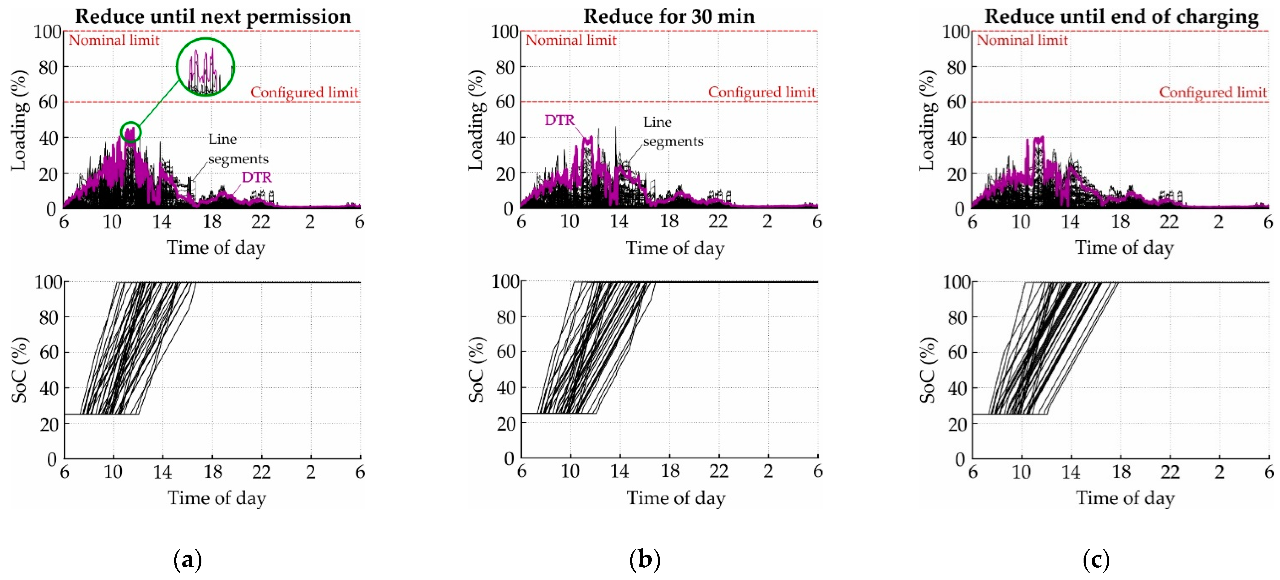
Figure 13 shows the loadings of the DTR and all line segments as well as the SoCs of all EV batteries for the scenario ‘Simultaneous charging in the evening’ with coordination and different algorithms at the EVCS level. Updating the internal charging power restrictions of EVCS each time new permissions are received provokes fluctuating power consumptions, which increase the SoCs of the corresponding EV batteries with an alternating gradient (Figure 13a, at the bottom). As the consequence, the LV equipment loading oscillates in the evening hours, causing numerous short-term violations of the configured DTR and feeder loading limits between 18:26 and 20:09 (Figure 13a, at the top). The corresponding energy losses and the average charging time per EV amount to 44.54 kWh and 233.43 min, respectively.
If charging with maximal power is allowed only when the permission is true for at least 30 minutes, the related power consumptions fluctuate slowly, leading to low-frequency oscillations of the LV equipment loading, Figure 13b. Four loading peaks occur that violate the configured loading limits. In this case, the energy losses and average charging time reach 39.38 kWh and 273.89 min, respectively. In Figure 13c, where the receipt of false permission reduces the power until the EV battery is fully charged, the loading limits are satisfied throughout the whole day. Energy losses are reduced to 37.80 kWh by prolonging the average charging time to 285.50 min.
3.2.2. Simultaneous Charging in the Morning
The loadings of the DTR and all line segments, as well as the SoCs of all EV batteries for the scenario ‘Simultaneous charging in the morning’ with coordination and different algorithms in the EVCS level, are shown in Figure 14. All algorithms eliminate the short-term violation of the configured loading limit that occurs without any coordination, Figure 9b. As in the previously described scenario, the application of the EVCS-internal algorithm ‘Reduce until next permission’ provokes significant oscillations of the DTR and line segment loadings around noon, Figure 14a. The EV batteries are charged with fluctuating power between 7:17 and 16:41 with an average charging time of 248.11 min, leading to energy losses of 16.15 kWh within the grid.
In Figure 14b, where the charging power is reduced for 30 min whenever false permission is received, the gradient of the SoC-curves changes less often than in Figure 14a. The oscillation of the equipment loading has a lower frequency, and some spikes have a higher magnitude. All charging processes are terminated at 16:51, yielding an average charging time of 279.74 min, and energy losses of 15.19 kWh. When the algorithm ‘Reduce until end of charging’ is applied, the charging power of each EVCS and thus the gradient of the corresponding SoC-curve changes one time at most, thus no oscillation of the equipment loading occurs, Figure 14c. In this case, the average charging time is increased to 287.04 min, and the losses are decreased to 14.76 kWh.
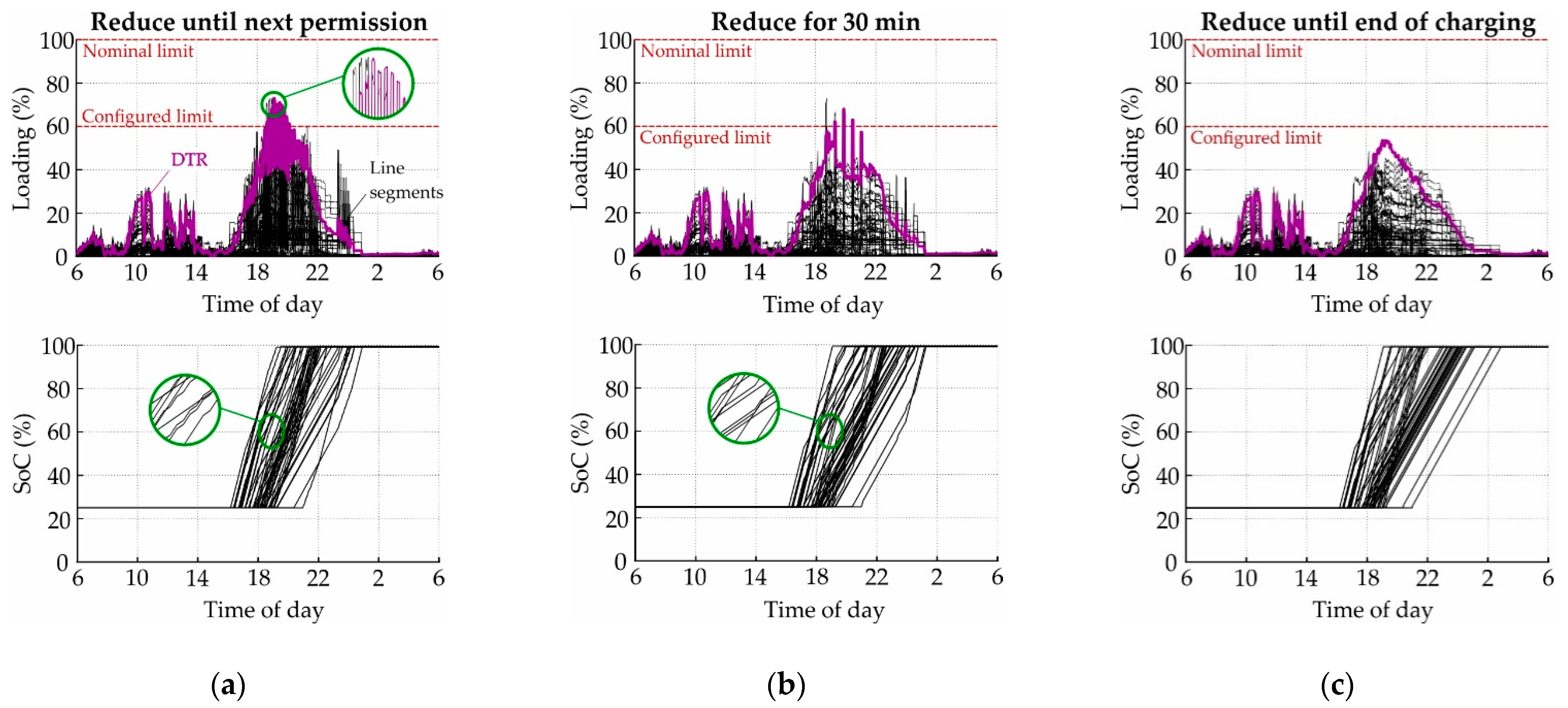
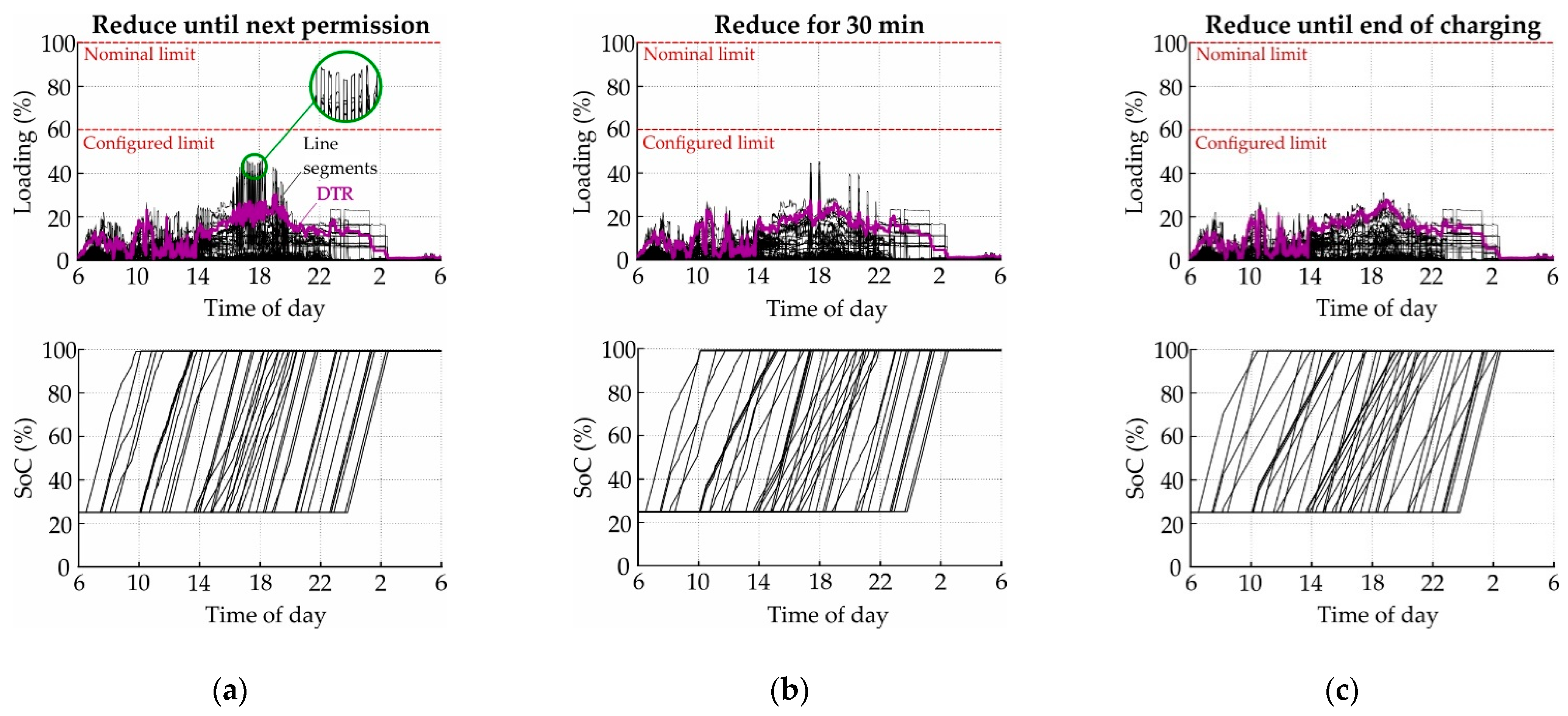
3.2.3. Charging throughout the Day
Figure 15 shows the loadings of the DTR and all line segments as well as the SoCs of all EV batteries for the scenario ‘Charging throughout the day’ with coordination and different algorithms at the EVCS level. Although the configured loading limits are not violated when no coordination is applied (see Figure 11b), all algorithms reduce the charging power of some EVCSs. Figure 15a shows significant oscillations of the DTR and line segment loadings, as well as SoC-curves with fast-changing gradients. The average charging time per EV battery and the energy losses amount to 183.41 min and 21.00 kWh in this case.
Considerably fewer spikes of the equipment loadings occur when a false permission reduces the charging power for 30 min, Figure 15b. The charging power changes less often, increasing the average charging time to 213.24 min, and reducing the losses to 20.31 kWh. Reducing the power for the complete charging process as soon as a false permission is received eliminates the loading oscillations, Figure 15c. The result is an average charging time of 233.59 min and energy losses of 19.63 kWh.
4. Discussion
The simulation results provide deep insights into the performances of both the method for the sparse measurement-based detection of feeder congestions and the coordination algorithms.
4.1. Sparse Measurement-Based Detection of Feeder Congestions
In the simulated cases, the proposed method for the sparse measurement-based detection of feeder congestions reliably identifies all overload situations. However, the worst-case assumptions made for the feeder structure (see Section 2.1.1) and the reactive power contribution of the PV systems (see Equation (11)) provoke a too conservative assessment of the grid state. As a consequence, overloads are detected in some situations in which actually no congestions are present, impairing the accuracy of the concept. Table 3 summarizes the detection accuracy values for the simulated scenarios without any coordination and for estimated and exact PV production. The proposed method detects congestions in low voltage feeders with the minimal accuracy of 73.07%. This value can be increased to 79.67% by improving the estimation of PV production.
One-hundred percent accuracy is reached for feeders 2, 5, and 6; they differ from the other feeders by their relatively low number of connected CPs with EVCS and PV systems (see Table 1). Feeder 4, which connects the most CPs and has the greatest total line length, yields the worst detection accuracy on average. However, no clear relation between the detection accuracy and the feeder properties—including cable share, maximal feeder length, total line length, the total number of connected CPs, and a number of connected CPs with EVCS and PV systems—can be observed from the simulation results. While improving the estimation of the PV production also improves the detection accuracy, no clear trend prevails for the dependency between detection accuracy and the time and simultaneity of EV charging.
4.2. CoordinationAalgorithms
The presented algorithms for the coordination of EVCSs modify the loading of the LV equipment by manipulating the SoC-curves of the EV batteries. In further consequence, this affects the energy losses of the grid and the average charging time per battery. As the permissions are specified without conducting any load flow simulations, their impact on the resulting system state is unknown in advance, giving the concept a “try-out and observe” character. In principle, this strategy is applicable as lines and transformers endure short-term violations of their thermal limits without sustaining significant deterioration. The overall system behavior greatly differs between the investigated EVCS-internal algorithms and the simulated scenarios. The energy losses and the average charging time in all simulated setups are overviewed in Table 4. Each coordination algorithm prolongs the EV battery charging on average, which reduces the associated grid losses in further consequence.
Updating the EVCS-internal charging power restrictions each time new permissions are received provokes severe oscillations of the charging power and the LV equipment loading in all simulated scenarios. This behavior is to be interpreted as a large number of trials, which are observed to be inappropriate by the central controller in its next algorithm execution. Due to numerous intervals in which the EVCSs charge with maximal power, the resulting average charging time is—compared to the other algorithm options—relatively low, while the energy losses are relatively high. The number of trials is significantly decreased when a delay of 30 minutes is implemented in the algorithm, reducing the frequency of the oscillations. This prolongs the periods of charging with minimal power, thus increasing the average charging time and reducing the associated losses. When the charging power is reduced until the end of the charging process as soon as dictated by the central controller, the oscillations are completely avoided. The maximal average charging time and the lowest energy loss is calculated for this case.
The algorithms ‘reduce until next permission’ and ‘reduce for 30 min’ are not sufficient to eliminate the violations of the configured loading limits when the customers simultaneously charge their EV batteries in the evening hours. If the simultaneity is relatively low and no limit violations appear at all, all algorithms reduce the charging power of at least some EVCSs unnecessarily. Reducing the power consumption until the corresponding battery is fully charged is the only option that establishes compliance to the configured loading limits in all simulated cases.
4.3. Applicability of the Concept
The state-of-art high-performance coordination schemes require sufficient numbers of sensors and detailed models of the low voltage feeders to conduct load flow calculations or to execute the DSSE. Furthermore, they impose considerable requirements on the communication infrastructure. In contrast, the presented solution is suboptimal but easy-to-implement and broadly applicable. It can be implemented for each LV grid with relatively low effort, regardless of its detailed structure. After grid expansion and reinforcement, no complex adaptation of the algorithm is required to maintain its functionality. Furthermore, the decisions of the algorithm can be documented and included in the reinforcement planning process: a large number of charging power reductions indicates the necessity of feeder reinforcement.
5. Conclusions
The proposed method for the sparse measurement-based detection of feeder congestions reliably identifies all overloads. Due to the worst-case assumptions underlying the concept, the assessment of the grid state is too conservative. Therefore, overloads are detected in some situations where actually no congestions are present. However, in the conducted simulations, the detection accuracy ranges from 73.07% to 100% when the PV production is estimated, and from 79.67% to 100% when it is well known.
The investigated coordination algorithms differently affect the LV equipment loading and energy losses, and the charging times of the electric vehicle batteries. All of them increase the charging times on average and decrease the associated grid losses. Waiving state estimation and load flow calculations to specify the charging permissions makes the proposed solution easy-to-implement but suboptimal: the use of the too conservative approach to detect feeder congestions may lead to an unnecessary reduction of the charging power; the “try out and observe” character may cause temporary violations of the configured loading limits, which may oscillate when the charging stations adapt their charging power according to the actual permission without significant delay. The most reliable but also conservative approach under consideration is to reduce the power absorbed by the electric vehicle charging station until the corresponding battery is fully charged as soon as congestion of the supplying feeder is detected.
The introduced solution is easy-to-implement and broadly applicable. It can be applied to any low voltage grid—regardless of its detailed structure—with relatively low effort on modeling and monitoring. No complex adaptations of the algorithms are required after grid reinforcement and expansion.
Funding
This research was funded by the Austrian Research Promotion Agency (FFG) and the Austrian Climate and Energy Fund (KLIEN), grant number 867276. Open Access Funding by TU Wien.
Data Availability Statement
Data is contained within the article.
Acknowledgments
The author acknowledges Alfred Einfalt for the practically orientated discussions that motivated the author to develop suboptimal but easy-to-implement solutions.
Conflicts of Interest
The author declares no conflict of interest. The funders had no role in the design of the study; in the collection, analyses, or interpretation of data; in the writing of the manuscript, or in the decision to publish the results.
Appendix A
Table A1 lists the used abbreviations and the corresponding full forms.

Table A1.
Abbreviations and corresponding full forms.
| CP | Customer Plant | EVCS | Electric Vehicle Charging Station |
| DER | Distributed energy resource | LF | Load flow |
| Dev | Device | LV | Low voltage |
| DSO | Distribution system operator | OLTC | On-load tap changer |
| DSSE | Distribution system state estimation | Pr | Producer |
| DTR | Distribution transformer | PV | Photovoltaic |
| EV | Electric vehicle | St | Storage |
Table A2 lists the nomenclature of the used variables.
Table A2.
Nomenclature of variables.
| Active and reactive power flows at the beginning of feeder f. | |
| Active and reactive power contributions of CP i connected to feeder f. | |
| Active and reactive power losses in the series impedances of all line segments of feeder f. | |
| Reactive power production of the shunt capacitances of all line segments of feeder f. | |
| Aggregate active and reactive power injections into feeder f. | |
| Minimal voltage of feeder f. | |
| Minimal thermal limit current of all line segments of feeder f. | |
| Voltage at the primary bus bar of the DTR. | |
| Voltage at the secondary bus bar of the DTR. | |
| Active and reactive power injections at the beginning of feeder f. | |
| Active and reactive power injections of CP i connected to feeder f. | |
| Number of customer plants connected to feeder f. | |
| Number of feeders. | |
| Estimated value of the maximum line segment loading of feeder f. | |
| Congestion flag related to feeder f. | |
| Apparent power injection at the beginning of feeder f. | |
| Limit of the line segment loading of feeder f. | |
| Thermal limit current of line segment , which is part of the main strands of feeder . | |
| Voltage measurement at feeder . | |
| Aggregate active and reactive power contributions of all consuming devices included in CP i connected to feeder f. | |
| Aggregate active and reactive power contributions of all producers included in CP i connected to feeder f. | |
| Aggregate active and reactive power contributions of all storages included in CP i connected to feeder f. | |
| Maximal active and reactive power injections of the producer included in CP i connected to feeder f. | |
| Rated apparent power of the distribution transformer. | |
| Loading of the distribution transformer. | |
| Congestion flag related to the distribution transformer. | |
| Limit of the distribution transformer loading. | |
| Active and reactive power contributions of the device model included in CP i connected to feeder f for nominal supply voltage. | |
| Normalized supply voltage of CP i connected to feeder f. | |
| Supply voltage of CP i connected to feeder f. | |
| State-of-charge of the electric vehicle battery included in CP i connected to feeder f. | |
| Active power contribution of the storage model included in CP i connected to feeder f for nominal supply voltage. | |
| Resolution of the load profiles. | |
| Storage capacity of the electric vehicle battery included in CP i connected to feeder f. | |
| Instant of time. | |
| Instant of time in which the charging process of the electric vehicle battery included in CP i connected to feeder f is started. | |
| Energy loss of the complete low voltage grid. | |
| Average charging time per electric vehicle battery. | |
| Active power loss of the distribution transformer. | |
| Active power loss of the line segment l. | |
| Charging time of electric vehicle charging station e. | |
| Number of electric vehicle charging stations. | |
| Number of instants of time in which the congestion flag related to feeder f is correctly set. | |
| Number of simulated instants of time. | |
| Detection accuracy related to feeder f. |
References
- Ilo, A.; Gawlik, W. The Way from Traditional to Smart Power Systems. In Proceedings of the IEWT 2015, Vienna, Austria, 11–13 February 2015. [Google Scholar]
- Sun, H.; Guo, Q.; Qi, J.; Ajjarapu, V.; Bravo, R.; Chow, J.H.; Li, Z.; Moghe, R.; Nasr, E.; Tamrakar, U.; et al. Review of Challenges and Research Opportunities for Voltage Control in Smart Grids. IEEE Trans. Power Syst. 2019, 34, 2790–2801. [Google Scholar] [CrossRef] [Green Version]
- Katiraei, F.; Aguero, J.R. Solar PV Integration Challenges. IEEE Power Energy Mag. 2011, 9, 62–71. [Google Scholar] [CrossRef]
- Nappu, M.B.; Arief, A.; Bansal, R.C. Transmission management for congested power system: A review of concepts, technical challenges and development of a new methodology. Renew. Sustain. Energy Rev. 2014, 38, 572–580. [Google Scholar] [CrossRef]
- Yilmaz, M.; Krein, P.T. Review of the Impact of Vehicle-to-Grid Technologies on Distribution Systems and Utility Interfaces. IEEE Trans. Power Electron. 2013, 28, 5673–5689. [Google Scholar] [CrossRef]
- Kundur, P. Reactive power and voltage control. In Power System Stability and Control, 1st ed.; Balu, N.J., Lauby, M.G., Eds.; McGraw-Hill Inc.: New York, NY, USA, 1994; pp. 627–687. [Google Scholar]
- Pillay, A.; Karthikeyan, S.P.; Kothari, D. Congestion management in power systems—A review. Int. J. Electr. Power Energy Syst. 2015, 70, 83–90. [Google Scholar] [CrossRef]
- Sarimuthu, C.R.; Ramachandaramurthy, V.K.; Agileswari, K.; Mokhlis, H. A review on voltage control methods using on-load tap changer transformers for networks with renewable energy sources. Renew. Sustain. Energy Rev. 2016, 62, 1154–1161. [Google Scholar] [CrossRef]
- Marggraf, O.; Laudahn, S.; Engel, B.; Lindner, M.; Aigner, C.; Witzmann, R.; Schoeneberger, M.; Patzack, S.; Vennegeerts, H.; Cremer, M.; et al. U-Control—Analysis of Distributed and Automated Voltage Control in current and future Distribution Grids. In Proceedings of the International ETG Congress 2017, Bonn, Germany, 28–29 November 2017. [Google Scholar]
- Ilo, A.; Schultis, D.-L.; Schirmer, C. Effectiveness of Distributed vs. Concentrated Volt/Var Local Control Strategies in Low-Voltage Grids. Appl. Sci. 2018, 8, 1382. [Google Scholar] [CrossRef] [Green Version]
- Rossi, M.; Viganò, G.; Moneta, D.; Clerici, D.; Carlini, C. Analysis of active power curtailment strategies for renewable distributed generation. In Proceedings of the 2016 AEIT International Annual Conference (AEIT), Capri, Italy, 5–7 October 2016; pp. 1–6. [Google Scholar]
- Li, B.; Chen, M.; Cheng, T.; Li, Y.; Hassan, M.A.S.; Xu, R.; Chen, T. Distributed Control of Energy-Storage Systems for Voltage Regulation in Distribution Network with High PV Penetration. In Proceedings of the 2018 UKACC 12th International Conference on Control (CONTROL), Sheffield, UK, 5–7 September 2018; pp. 169–173. [Google Scholar]
- Clement-Nyns, K.; Haesen, E.; Driesen, J. The Impact of Charging Plug-In Hybrid Electric Vehicles on a Residential Distribution Grid. IEEE Trans. Power Syst. 2009, 25, 371–380. [Google Scholar] [CrossRef] [Green Version]
- Deilami, S.; Masoum, A.S.; Moses, P.S.; Masoum, M.A.S. Real-Time Coordination of Plug-In Electric Vehicle Charging in Smart Grids to Minimize Power Losses and Improve Voltage Profile. IEEE Trans. Smart Grid 2011, 2, 456–467. [Google Scholar] [CrossRef]
- Ilo, A.; Prata, R.; Strbac, G.; Giannelos, S.; Bissell, G.R.; Kulmala, A.; Constantinescu, N.; Samovich, N.; Iliceto, A. Holistic Architectures for Future Power Systems. ETIP SNET White Paper. 2019. Available online: https://www.etip-snet.eu/etip_publ/white-paper-holistic-architectures-future-power-systems/ (accessed on 22 December 2020).
- Ilo, A. Use cases in Sector Coupling as part of the LINK-based holistic architecture to increase the grid flexibility. In Proceedings of the CIRED 2020 Berlin Workshop, Berlin, Germany, 22–23 September 2020. [Google Scholar]
- Ilo, A. “Link”—The smart grid paradigm for a secure decentralized operation architecture. Electr. Power Syst. Res. 2016, 131, 116–125. [Google Scholar] [CrossRef]
- Veetil, V.P. Coordination in Centralized and Decentralized Systems. Int. J. Microsimulation 2017, 10, 86–102. [Google Scholar] [CrossRef]
- Schweppe, F.C.; Wildes, J. Power System Static-State Estimation, Part I: Exact Model. IEEE Trans. Power Appar. Syst. 1970, 1, 120–125. [Google Scholar] [CrossRef] [Green Version]
- Primadianto, A.; Lu, C.-N. A Review on Distribution System State Estimation. IEEE Trans. Power Syst. 2016, 32, 3875–3883. [Google Scholar] [CrossRef]
- Ahmad, F.; Rasool, A.; Ozsoy, E.; Sekar, R.; Sabanovic, A.; Elitaş, M. Distribution system state estimation-A step towards smart grid. Renew. Sustain. Energy Rev. 2018, 81, 2659–2671. [Google Scholar] [CrossRef] [Green Version]
- Siano, P. Demand response and smart grids—A survey. Renew. Sustain. Energy Rev. 2014, 30, 461–478. [Google Scholar] [CrossRef]
- Hu, J.; You, S.; Lind, M.; Ostergaard, J. Coordinated Charging of Electric Vehicles for Congestion Prevention in the Distribution Grid. IEEE Trans. Smart Grid 2014, 5, 703–711. [Google Scholar] [CrossRef] [Green Version]
- Bhattarai, B.P.; Bak-Jensen, B.; Pillai, J.R.; Mahat, P. Two-stage electric vehicle charging coordination in low voltage distribution grids. In Proceedings of the 2014 IEEE PES Asia-Pacific Power and Energy Engineering Conference (APPEEC), Hong Kong, China, 7–10 December 2014; pp. 1–5. [Google Scholar]
- Sundstrom, O.; Binding, C. Flexible Charging Optimization for Electric Vehicles Considering Distribution Grid Constraints. IEEE Trans. Smart Grid 2011, 3, 26–37. [Google Scholar] [CrossRef]
- Dixon, J.; Bukhsh, W.; Edmunds, C.; Bell, K. Scheduling electric vehicle charging to minimise carbon emissions and wind curtailment. Renew. Energy 2020, 161, 1072–1091. [Google Scholar] [CrossRef]
- Schultis, D.-L. Coordinated electric vehicle charging—Performance analysis of developed algorithms. In Proceedings of the CIRED 2021 Conference, Geneva, Switzerland, 21–24 June 2021. [Google Scholar]
- Einfalt, A.; Brunner, H.; Pruggler, W.; Schultis, D.-L.; Herbst, D.; Beidinger, T.; Hauer, D.; Lugmaier, A. Efficient utilisation of existing grid infrastructure empowering smart communities. In Proceedings of the 2020 IEEE Power & Energy Society Innovative Smart Grid Technologies Conference (ISGT), Washington, DC, USA, 17–20 February 2020; pp. 1–5. [Google Scholar]
- Strunz, K. Benchmark Systems for Network Integration of Renewable and Distributed Energy Resources. Cigre Task Force C 2014, 6, 78. [Google Scholar]
- Schultis, D.-L.; Ilo, A. Adaption of the Current Load Model to Consider Residential Customers Having Turned to LED Lighting. In Proceedings of the 2019 IEEE PES Asia-Pacific Power and Energy Engineering Conference (APPEEC), Macao, China, 1–4 December 2019. [Google Scholar]
- IEEE. IEEE Standard for Interconnection and Interoperability of Distributed Energy Resources with Associated Electric Power Systems Interfaces; IEEE: New York, NY, USA, 2018; pp. 1–138. [Google Scholar]
- Leemput, N.; Geth, F.; Van Roy, J.; Büscher, J.; Driesen, J. Reactive power support in residential LV distribution grids through electric vehicle charging. Sustain. Energy, Grids Netw. 2015, 3, 24–35. [Google Scholar] [CrossRef]
- Wang, J.; Bharati, G.R.; Paudyal, S.; Ceylan, O.; Bhattarai, B.P.; Myers, K.S. Coordinated Electric Vehicle Charging With Reactive Power Support to Distribution Grids. IEEE Trans. Ind. Inform. 2019, 15, 54–63. [Google Scholar] [CrossRef]
- Antonanzas, J.; Osorio, N.; Escobar, R.; Urraca, R.; Martinez-De-Pison, F.J.; Antonanzas-Torres, F. Review of photovoltaic power forecasting. Sol. Energy 2016, 136, 78–111. [Google Scholar] [CrossRef]
- Schultis, D.-L.; Ilo, A.; Schirmer, C. Overall performance evaluation of reactive power control strategies in low voltage grids with high prosumer share. Electr. Power Syst. Res. 2019, 168, 336–349. [Google Scholar] [CrossRef]
- Schultis, D.-L. Comparison of Local Volt/var Control Strategies for PV Hosting Capacity Enhancement of Low Voltage Feeders. Energies 2019, 12, 1560. [Google Scholar] [CrossRef] [Green Version]
- Bokhari, A.; Alkan, A.; Dogan, R.; Diaz-Aguilo, M.; De Leon, F.; Czarkowski, D.; Zabar, Z.; Birenbaum, L.; Noel, A.; Uosef, R.E. Experimental Determination of the ZIP Coefficients for Modern Residential, Commercial, and Industrial Loads. IEEE Trans. Power Deliv. 2014, 29, 1372–1381. [Google Scholar] [CrossRef]
- Shukla, A.; Verma, K.; Kumar, R. Multi-stage voltage dependent load modelling of fast charging electric vehicle. In Proceedings of the 2017 6th International Conference on Computer Applications In Electrical Engineering-Recent Advances (CERA), Roorkee, India, 5–7 October 2017; pp. 86–91. [Google Scholar]
- Load Profile Generator. Available online: https://www.loadprofilegenerator.de/ (accessed on 20 November 2020).
- McKenna, E.; Thomson, M.; Barton, J. CREST Demand Model; Data Set; Loughborough University: Loughborough, UK, 2015. [Google Scholar] [CrossRef]
Figure 1.
Structure of low voltage grids: (a) detailed; (b) simplified.

Figure 2.
Current flows through a low voltage (LV) feeder with main and side strands.

Figure 3.
Suggested placement of measurement devices on one representative real LV feeder.

Figure 4.
Overview of the coordination algorithms executed by different devices: (a) central controller; (b) different options for the distributed electric vehicle charging stations (EVCSs).
Figure 4.
Overview of the coordination algorithms executed by different devices: (a) central controller; (b) different options for the distributed electric vehicle charging stations (EVCSs).

Figure 5.
Power system model: (a) simplified one-line diagram of the LV grid; (b) customer plants (CP) structure.
Figure 5.
Power system model: (a) simplified one-line diagram of the LV grid; (b) customer plants (CP) structure.

Figure 6.
Load profiles of different CP components: (a) device (Dev)-model; (b) producer (Pr)-model.
Figure 6.
Load profiles of different CP components: (a) device (Dev)-model; (b) producer (Pr)-model.

Figure 7.
Simulation results for the scenario ‘Simultaneous charging in the evening’ without any coordination: (a) SoCs of all EV batteries; (b) equipment loading; (c) grid state at 18:46.
Figure 7.
Simulation results for the scenario ‘Simultaneous charging in the evening’ without any coordination: (a) SoCs of all EV batteries; (b) equipment loading; (c) grid state at 18:46.

Figure 8.
Line segment loadings and congestion flag of different feeders for the scenario ‘Simultaneous charging in the evening’ without any coordination.
Figure 8.
Line segment loadings and congestion flag of different feeders for the scenario ‘Simultaneous charging in the evening’ without any coordination.

Figure 9.
Simulation results for the scenario ‘Simultaneous charging in the morning’ without any coordination: (a) SoCs of all EV batteries; (b) equipment loading; (c) grid state at 10:33.
Figure 9.
Simulation results for the scenario ‘Simultaneous charging in the morning’ without any coordination: (a) SoCs of all EV batteries; (b) equipment loading; (c) grid state at 10:33.

Figure 10.
Line segment loadings and congestion flag of different feeders for the scenario ‘Simultaneous charging in the morning’ without any coordination.
Figure 10.
Line segment loadings and congestion flag of different feeders for the scenario ‘Simultaneous charging in the morning’ without any coordination.

Figure 11.
Simulation results for the scenario ‘Charging throughout the day’ without any coordination: (a) SoCs of all EV batteries; (b) equipment loading; (c) grid state at 16:47.
Figure 11.
Simulation results for the scenario ‘Charging throughout the day’ without any coordination: (a) SoCs of all EV batteries; (b) equipment loading; (c) grid state at 16:47.

Figure 12.
Line segment loadings and congestion flag of different feeders for the scenario ‘Charging throughout the day’ without any coordination.
Figure 12.
Line segment loadings and congestion flag of different feeders for the scenario ‘Charging throughout the day’ without any coordination.

Figure 13.
LV equipment loading and SoCs of all EV batteries for the scenario ‘Simultaneous charging in the evening’ with coordination and different algorithms in EVCS level: (a) reduce until next permission; (b) reduce for 30 min; (c) reduce until end of charging.
Figure 13.
LV equipment loading and SoCs of all EV batteries for the scenario ‘Simultaneous charging in the evening’ with coordination and different algorithms in EVCS level: (a) reduce until next permission; (b) reduce for 30 min; (c) reduce until end of charging.

Figure 14.
LV equipment loading and SoCs of all EV batteries for the scenario ‘Simultaneous charging in the morning’ with coordination and different algorithms in EVCS level: (a) reduce until next permission; (b) reduce for 30 min; (c) reduce until end of charging.
Figure 14.
LV equipment loading and SoCs of all EV batteries for the scenario ‘Simultaneous charging in the morning’ with coordination and different algorithms in EVCS level: (a) reduce until next permission; (b) reduce for 30 min; (c) reduce until end of charging.

Figure 15.
LV equipment loading and SoCs of all EV batteries for the scenario ‘Charging throughout the day’ with coordination and different algorithms in EVCS level: (a) reduce until next permission; (b) reduce for 30 min; (c) reduce until end of charging.
Figure 15.
LV equipment loading and SoCs of all EV batteries for the scenario ‘Charging throughout the day’ with coordination and different algorithms in EVCS level: (a) reduce until next permission; (b) reduce for 30 min; (c) reduce until end of charging.

Table 1.
Feeder-related data of the LV grid model.
| Feeder | Cable Share in % | Maximal Feeder Length in km | Total Line Length in km | Number of Connected CPs | |
|---|---|---|---|---|---|
| In Total | With EVCS and PV System | ||||
| 1 | 51.92 | 0.49 | 1.040 | 26 | 10 |
| 2 | 100 | 0.15 | 0.205 | 4 | 3 |
| 3 | 100 | 0.43 | 0.810 | 18 | 9 |
| 4 | 93.55 | 0.61 | 1.550 | 23 | 15 |
| 5 | 100 | 0.27 | 0.490 | 7 | 3 |
| 6 | 61.36 | 0.61 | 0.880 | 13 | 6 |
Table 2.
Overview of all conducted simulations.
| Scenario | Coordination Algorithm | |
|---|---|---|
| Central Controller | Distributed EVCSs | |
| Simultaneous charging in the evening | None | None |
| Specify permissions | Reduce until next permission | |
| Reduce for 30 min | ||
| Reduce until end of charging | ||
| Simultaneous charging in the morning | None | None |
| Specify permissions | Reduce until next permission | |
| Reduce for 30 min | ||
| Reduce until end of charging | ||
| Charging throughout the day | None | None |
| Specify permissions | Reduce until next permission | |
| Reduce for 30 min | ||
| Reduce until end of charging | ||
Table 3.
Accuracy of the sparse measurement-based detection of feeder congestions.
| PV Production | Scenario | Detection Accuracy by the Feeder in % | |||||
|---|---|---|---|---|---|---|---|
| 1 | 2 | 3 | 4 | 5 | 6 | ||
| Estimated | Simultaneous charging in the evening | 92.92 | 100 | 89.11 | 81.26 | 100 | 100 |
| Simultaneous charging in the morning | 91.46 | 100 | 81.54 | 77.17 | 100 | 100 | |
| Charging throughout the day | 100 | 100 | 89.45 | 73.07 | 100 | 100 | |
| Exact | Simultaneous charging in the evening | 92.92 | 100 | 89.11 | 82.03 | 100 | 100 |
| Simultaneous charging in the morning | 97.57 | 100 | 88.27 | 79.67 | 100 | 100 | |
| Charging throughout the day | 100 | 100 | 100 | 87.30 | 100 | 100 | |
Table 4.
Energy losses in the LV grid and average charging time per EV battery.
| Scenario | Coordination Algorithm | Energy Loss in kWh | Average Charging Time in min | |
|---|---|---|---|---|
| Central Controller | Distributed EVCSs | |||
| Simultaneous charging in the evening | None | None | 56.65 | 161.00 |
| Specify permissions | Reduce until next permission | 44.54 | 233.43 | |
| Reduce for 30 min | 39.38 | 273.89 | ||
| Reduce until end of charging | 37.80 | 285.50 | ||
| Simultaneous charging in the morning | None | None | 22.28 | 161.00 |
| Specify permissions | Reduce until next permission | 16.15 | 248.11 | |
| Reduce for 30 min | 15.19 | 279.74 | ||
| Reduce until end of charging | 14.76 | 287.04 | ||
| Charging throughout the day | None | None | 21.31 | 161.00 |
| Specify permissions | Reduce until next permission | 21.00 | 183.41 | |
| Reduce for 30 min | 20.31 | 213.24 | ||
| Reduce until end of charging | 19.63 | 233.59 | ||
Publisher’s Note: MDPI stays neutral with regard to jurisdictional claims in published maps and institutional affiliations. |
© 2020 by the author. Licensee MDPI, Basel, Switzerland. This article is an open access article distributed under the terms and conditions of the Creative Commons Attribution (CC BY) license (http://creativecommons.org/licenses/by/4.0/).
Share and Cite
MDPI and ACS Style
Schultis, D.-L. Sparse Measurement-Based Coordination of Electric Vehicle Charging Stations to Manage Congestions in Low Voltage Grids. Smart Cities 2021, 4, 17-40. https://0-doi-org.brum.beds.ac.uk/10.3390/smartcities4010002
AMA Style
Schultis D-L. Sparse Measurement-Based Coordination of Electric Vehicle Charging Stations to Manage Congestions in Low Voltage Grids. Smart Cities. 2021; 4(1):17-40. https://0-doi-org.brum.beds.ac.uk/10.3390/smartcities4010002
Chicago/Turabian StyleSchultis, Daniel-Leon. 2021. "Sparse Measurement-Based Coordination of Electric Vehicle Charging Stations to Manage Congestions in Low Voltage Grids" Smart Cities 4, no. 1: 17-40. https://0-doi-org.brum.beds.ac.uk/10.3390/smartcities4010002