Article

From Conventional to Precision Fertilization: A Case Study on the Transition for a Small-Medium Farm

1
Consiglio per la Ricerca in Agricoltura e l’Analisi dell’Economia Agraria (CREA), Centro di Ricerca Ingegneria e Trasformazioni Agroalimentari, Via Milano, 43, 24047 Treviglio, Italy
2
Consiglio per la Ricerca in Agricoltura e l’Analisi dell’Economia Agraria (CREA), Centro di Ricerca Ingegneria e Trasformazioni Agroalimentari, Via della Pascolare 16, 00015 Monterotondo, Italy
3
Dipartimento di Scienze dell’Ambiente e della Terra, Università degli Studi di Milano Bicocca, P.zza della Scienza, 1, 20126 Milano, Italy
*
Author to whom correspondence should be addressed.
Submission received: 12 May 2021 / Revised: 10 June 2021 / Accepted: 11 June 2021 / Published: 16 June 2021
(This article belongs to the Special Issue Evaluation of New Technological Solutions in Agriculture)

Abstract

:
At the CREA research facility of Treviglio (Bergamo, Italy), to provide farmers with valuable hints for the transition from conventional to precision agriculture, information on crop production dynamics (Maize and Triticale) has been obtained using real-time soil mapping (resistivity technique) and production quality and quantity monitoring with a commercial yield mapping apparatus. The geostatistical processing of data resulted in the same zoning for Triticale, meaning that the characteristics of soil influenced crop behavior more than the variability resulting from other factors, which suggests that improvements in product yields can be planned and achieved acting, for instance, on variable rate distribution of fertilizers. The importance of the acquired data can help farmers to manage factors that are external to their plots of land.

1. Introduction

According to Precision Agriculture (P.A.) principles, managing arable lands means considering the inherent variability of the cultivation and that generated by external factors in such a way that both farmers’ profitability and environmental stewardship turn out to be increased [1,2,3]. Moreover, steady (or less variable) conditions, such as soil and boundary conditions, topography, hydrographic network, and their interactions with intrinsic variables, must be considered [4,5]. Farming tasks, i.e., cultivation, seeding, fertilization, herbicide application, and harvesting, can be carried out by linking the mapped variables to appropriate farming decisions. Thanks to Global Navigation Satellite System technology and sensors’ development, such actions can currently be carried out with improved accuracy, reduced energy needs, and better timeliness. In particular, sensors can be used both in-situ and on-the-go recording modes, which enables the site-specific knowledge of soil status (e.g., apparent electrical conductivity sensors, gamma-radiometric soil sensors, and soil moisture devices), weather information, and physiological status of crops (e.g., nitrogen sensors). At the same time, the acquisition of farm-level imagery allows the transformation of the collected geo-referenced data into maps that are helpful in setting up management plans aimed at increasing farming efficiency throughout the years. When concerning crop production, prescription mapping is essential: if, on the one hand, any plant needs water, nutrients, and carbon dioxide for its growth, on the other, soil heterogeneity and topography unavoidably affect the production dynamic [6].
Transitioning from conventional to precision agriculture practices requires farmers to adopt specific technology [7]. However, farmers are conservative, so increasing their trust in these technologies is essential in facilitating the new technology breakthrough [8,9]. Trust is built when users have a clear conception of the appliance’s functionality, even though they do not know all of the details [10]. Introducing guidelines aimed at promoting new agro technical patterns that are based on P.A. principles could help to strengthen the confidence of farmers: the parallel set up of applicative examples and references (the so-called Living Labs) could also foster the adoption of such guidelines [11].
Following the national public consultation on precision farming that the Italian Ministry of Agriculture [12] set up to increase overall farming sustainability, at the CREA research facility of Treviglio (Italy), precision farming trials have been carried out that introduced soil mapping, followed by harvest monitoring, as the first steps. In this work we focused on the steps required for the assessment of prescription maps to improve crop production in light of the in-field variability with a twofold objective: (i) setting up an appropriate management plan that enables overcoming the site-specific limiting factors and improving crop yield uniformity, (ii) providing farmers with valuable hints to help them in the transition from conventional to precision agriculture to go beyond state of the art.

2. Materials and Methods

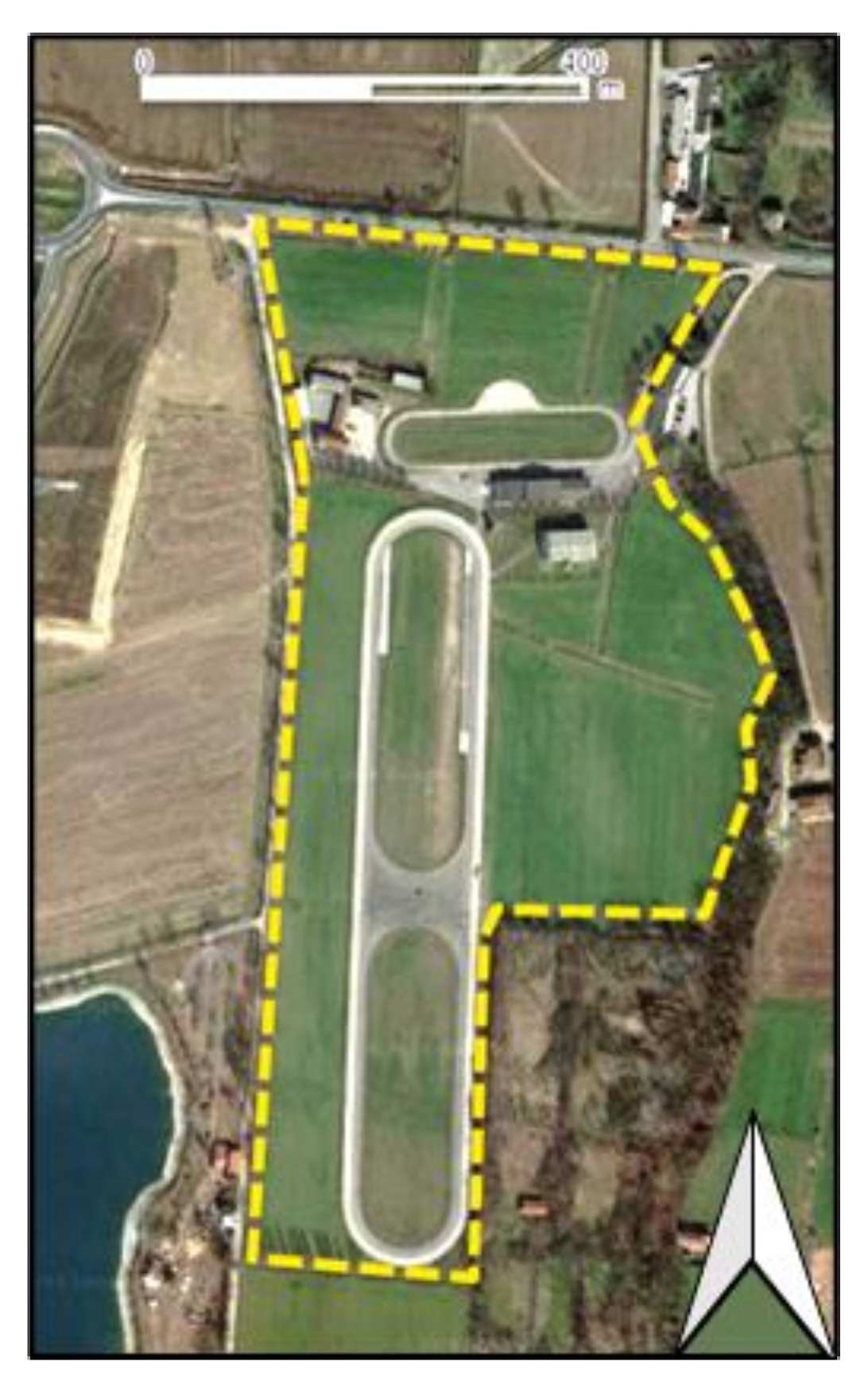
2.1. The Experimental Site

The CREA experimental site (Figure 1) is located in Treviglio, Northern Italy (45°31′14″ N; 9°35′27″ E; +128 m a.s.l.): it comprises two experimental tracks, one of which is flanked with 2.00 ha of soil for agriculture machinery and tires testing, and 10.00 ha of experimental fields that are sown with Triticale as winter crop (Triticosecale Wittnack) and Maize (Zea mays). According to World Reference Base for Soil Resources [13], the soil has been classified as Calcic Skeletic Mollic Umbrisol, with neutral-sub alkaline pH and generally carbonates being present from the surface. Before seeding Triticale and Maize, all of the agricultural surface underwent manuring treatment with 100 m3 ha−1 of dairy manure before ploughing and harrowing. Besides seeding, both of the crops were also fertilized with 250 kg ha−1 of urea (46% nitrogen content) when in the jointing phase.

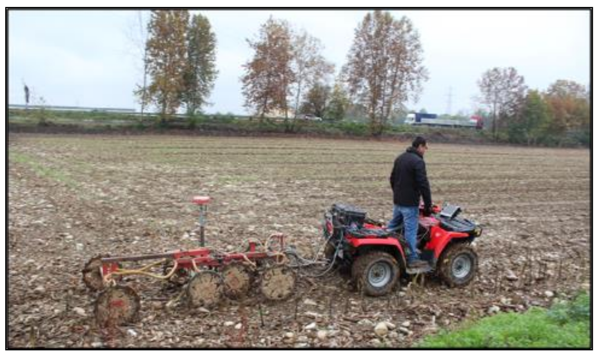
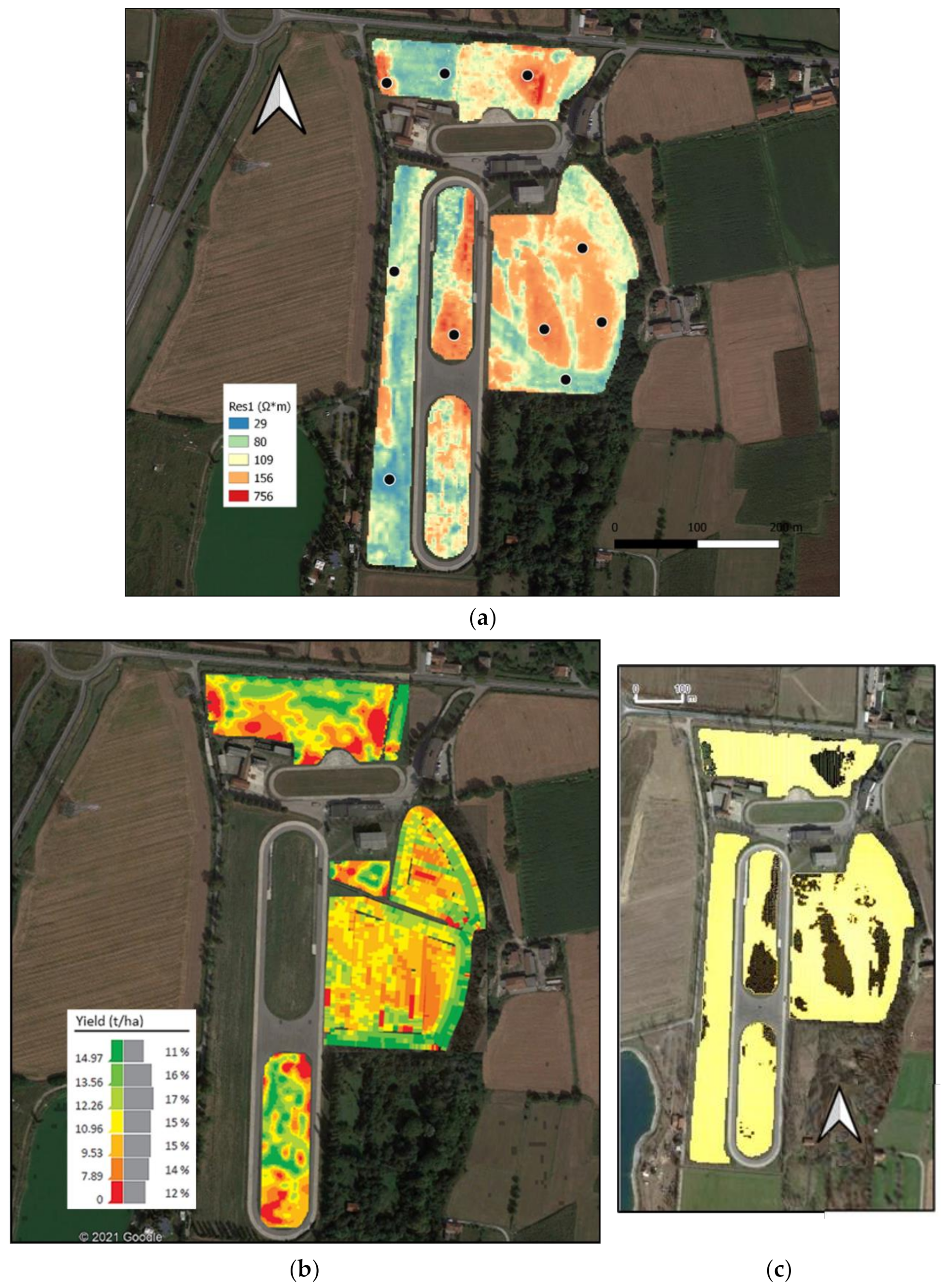
2.2. Soil Geophysical and Traditional Survey

A soil geophysical survey took place using the Automatic Resistivity Profiler (A.R.P.; Geocarta SA, Paris, France). It is a mobile system that consists of four pairs of toothed metal wheels. The first pair functions as injection electrodes, and the other three couples function as receivers, which measure the electrical potential difference (Figure 2). The distance between each pair of receivers was calibrated to investigate three depths (0–50 cm, 0–100 cm, and 0–180 cm).
The raw data were filtered using a 1D-median filter and then interpolated to obtain one soil resistivity map (2 × 2 m pixel) for each investigated layer. The locations of soil profiles investigations provided representative coverage of the resistivity values. Therefore, ten soil profiles were opened and described by horizons estimating, for each profile, the volumetric percentage of rock fragments in the 0–50 cm layer. From the 0–50 cm layer, soil samples were collected and analyzed to determine soil organic carbon (S.O.C.), pH in water (soil to water ratio of 1:2.5), particle-size distribution by sieving and sedimentation [14] (sand, 0.05–2 mm; silt, 0.002–0.05; clay, <0.002 mm), and available phosphorus [15].

2.3. Harvest Monitoring

Triticale and Maize were both harvested to produce silage: the forage harvester (John Deere, Moline, IL, USA) was equipped, alternatively, with maize and whole crop headers, which were both of 6 m working width. The dry matter yield per area unit resulted from the equipment of the harvester with a commercial yield mapping apparatus [16]. It consisted of a global positioning system (G.P.S.), a feed roll linear variable differential transformer sensor, a feed roll speed optical sensor, and a moisture measurement sensor. The working width considered for the calculation of the output was automatically set by the control system of the forager at intervals of 1.5 m. Such a device relates to speed measurements from the G.P.S. to estimate the wet yield per area. The moisture sensor measures moisture and dry matter (D.M.) using near-infrared spectroscopy. Being placed on the machine’s spout, it measures the crop D.M. and estimates the dry yield. It allowed for the realization of the yield maps by coupling crop biomass flow data with those from the G.P.S.

2.4. Data Processing

Data underwent geostatistical analysis using “R” statistical software [17] and the “Quantum GIS” (QGIS) software package [18]. Before geostatistical analysis, all of the coordinates that were retrieved by the instruments and mapping services were converted from geographic coordinates (World Geodetic System 84-WGS84) into UTM Cartesian coordinates using the “spTransform” function of the “ rgdal” package [19]. All of the statistical processing took place following the findings of Córdoba et al. [20]. Clustering occurred considering the interaction of the three layers of soil electrical resistivity data (Ω m) and the dry matter yield from the on-the-go sampling of the forage harvester (t ha−1) from the previous year (Figure 3b), and the indices were calculated to achieve the optimum number of clusters. Data visualization and editing were carried out using the QGIS software [21].

3. Results and Discussion

Soil apparent electrical resistivity (Figure 3a) is an important indicator that relates directly and indirectly to soil properties [22,23,24,25,26].
Figure 3a shows the resistivity map of the first layer of soil investigated.
The apparent resistivity values presented in this study were highly variable and in line with the findings of Hunt [27], who indicated that the electrical resistivity varies from minimal values (i.e., 1.5 Ω m and below) for wet clay soils to more than 2400 Ω m for massive and hard bedrocks. In this study, they ranged between 29 and 756 Ω m and resulted in being significantly related (p-value < 0.05) to soil properties, such as soil texture, rock fragment content, total carbonates, and available phosphorus (Table 1 and Table 2). When compared to the less resistive ones, the areas with high resistivity values showed higher rock fragment and total carbonates contents, coarser soil texture, and lower phosphorus content.
The geostatistical analysis tested various clustering solutions to give rise to the zoning of the farm fields. A good correlation exists between soil electrical resistivity and crop production characteristics (amounts and dry matter) when comparing the resulting maps (Figure 3b). Table 2 reports the statistical indices evaluated, which resulted in the clustering solution that is displayed in Figure 3c.
Various potential clustering options were tested during the geostatistical analysis, which evaluated the grouping into two, three, and four clusters to determine the most appropriate solution. Such a comparison pointed out that two was the optimum number of classes, because all of the considered indexes, i.e., the Xie–Beni [28], the Fukuyama-Sugeno [29], the Partition coefficient [30], and the Proportion Exponent [31], had the lowest value for that grouping (Table 3). The differences between the values of the indices obtained are comparable with those that were also obtained by Córdoba and Galarza [20,32]. According to this, the classification of the management zones means that the final output exhibits large zones with coherent boundaries that result in more straightforward management of the information than in the case of classifications having many small and irregular zones.
Therefore, the two-zone clustering has the advantage of obtaining more homogeneous management zones. In greater detail, the output of the analysis shows that, no matter the grown crop, soil characteristics and variability identify zones where the yield is significantly far from optimal (the black zones in Figure 3c), and this means that the decisions to be taken will necessarily involve the specific knowledge of the variables impairing the yield in such zones.
Furthermore, although the yield maps show that crop moisture was higher along the plot borders, which indicated a possible effect of the bordering uncultivated woody and shady areas, the analysis results showed that the spot presence of stony zones in the considered plots has a more remarkable effect on crop production.
The large percentage of stones strongly influenced the soil behavior in the black-colored zones. In addition, the soils of such zones are more sandy, more lacking in organic matter and available phosphorus, and they have more carbonates than those in the better areas: in short, they are less fertile. According to this, the utilization of specific manuring has been planned that employs a variable rate technology spreader that adapts and optimizes the amount of manure to be spread (and, afterwards, incorporated into the soil) according to the prescription map that result from this study with a subsequent real improvement of the soil environment, which makes it more suitable for plant growth.
According to some authors, soil-based maps cannot reproduce the actual yield levels, while crop monitoring can give rise to high accuracy, reliability, and discrimination ability management zone mapping [33]. The zoning approach suffers from the hypothesis that soil characteristics would dominate the effect on crop performance, resulting in relatively similar crop yield patterns each year. This assumption only works when the yield-limiting parameters are permanent [34,35]. Therefore, identifying subfield regions with homogeneous yield-limiting factors (homogeneous management zones) requires a deep understanding of field spatial variability and the interaction between the whole system of soil, crop, weather, and management practices (e.g., fertilizer, irrigation).
The method for preparing the prescription map used in this study considered the information from the resistivity that was observed in the three depths and from the previous year’s production map (Figure 3b). It should be noted that the areas of different management that resulted from the clustering could change their shape if the sources of information change and, therefore, can undergo continuous adaptation when, time after time, new information on the fields is available. Such a consideration is in line with the findings of Rodrigues et al. [36], who pointed out that the optimum number of management zones can change over time while applying and following the spatial-temporal variability of soil and corn yield,.
Furthermore, the methodology that was developed in this study envisaged following the protocol outlined by Córdoba [20] to determine the number of most appropriate clusters from a statistical point of view, i.e., according to the statistically significant difference between the points belonging to different clusters. On the one hand, the development of the analytical outline in R software (open source) makes it available for implementation and application, but, on the other, it requires specific statistical and coding expertise.
The comparison with reality sees clustering as very critical, because the determination of the clusters should also consider the technical means that are capable of supporting this choice. In the present case, the two clusters option, which is the optimal combination from a statistical point of view, is also optimal from a practical perspective. The P.A. machinery ordinarily agricultural contractors use, albeit being technologically upgraded, may encounter difficulties in following more complex (highly clustered) prescription maps, because neither the means of production nor the technical characteristics of the equipment available in the farm could support them. Therefore, it is appropriate to study methods that consider the detail that the statistical procedures can achieve and the precision level of the machinery to find a proper in-farm application combination. The resulting zoning (Figure 3c) resulted in being the same for Triticale and maize, which meant that the soil characteristics pointed outlined by A.R.P. do influence crop behavior more than the variability that is related to the crop itself.
Some studies recently examined the transfer schemes to incentivize the transition of farmers towards P.A. and enhance the ability of farmers to connect with the know-how, the networks, and the institutions to improve productivity [37,38]: our results (that are in line with their findings) allow farmers to overcome the initial standstill, and put transitioning towards P.A. into practice to gain experience and, in turn, complement the information from numerical and computational analysis [39].

4. Conclusions

The A.R.P. turned out to be a suitable surrogate for detailed and georeferred soil coring: cluster analysis of AR.P. and yield data provided an objective method to identify management zones for targeted sampling activities (e.g., soil nutrients, organic matter, pH, soil remediation, etc.), which enabled setting up and variable rate manure applications.
According to the results, improvements in product yields can be planned and achieved acting on variable rate distribution of fertilizers (manure in particular), while the bordering with uncultivated zones is of secondary importance.
The applied farm management information system allows for the management of high-value crops, efficiently increasing harvest quality and quantity, and helping farmers to make decisions. When transitioning to P.A., the optimized machinery enabling better matching of soil characteristics with crop requirements plays a key role: however, the importance of the acquirable data is not limited to the in-field variability, and it can also help farmers to manage factors from outside their plots of land.
The available information from the processing procedures always requires considering the technical means that are available at the farm level to find the most appropriate practical combination. Finally, the awareness of the optimized inputs is derived from the high quantity of information (mapping and sensing techniques) that could effectively integrate the farmers’ daily experience, which results in increasing perception and reception of precision farming.

Author Contributions

Conceptualization, M.B. (Massimo Brambilla), E.R., C.B. and R.C.; methodology, E.R., R.C.; software, E.R., C.F.; formal analysis, M.B. (Marcello Biocca) and M.C., investigation, P.T., E.R., R.C., C.F.; data curation, E.R., C.F., R.C.; writing—original draft preparation, M.B. (Massimo Brambilla) and M.C.; writing—review and editing, M.B. (Massimo Brambilla); supervision, C.B. and R.C.; project administration, C.B. and R.C.; funding acquisition, C.B. and R.C. All authors have read and agreed to the published version of the manuscript.

Funding

This work was supported by the Italian Ministry of Agriculture (MiPAAF) through the “AGROENER” project (Decree n. 26329, 1 April 2016) and the “AGRI DIGIT” Programme (Decree n. 2111-B/2015).

Institutional Review Board Statement

Not applicable.

Informed Consent Statement

Not applicable.

Data Availability Statement

Data sharing is not applicable to this article.

Acknowledgments

The authors would like to thank Roberto Negroni (Agromeccanica Negroni srl, Stezzano, Italy), who provided the geo-referenced yield data and Elia Premoli and Alex Filisetti of the CREA-IT experimental farm of Treviglio (BG), Italy for the setup of the research and data collection.

Conflicts of Interest

The authors declare no conflict of interest. The funders had no role in the design of the study; in the collection, analyses, or interpretation of data; in the writing of the manuscript, or in the decision to publish the results.

List of Acronyms

P.A.Precision Agriculture
A.R.P.Automatic Resistivity Profiler
G.P.S.Global positioning system
D.M.Dry Matter
QGISQuantum Gis
CaCO3Total Carbonates;
PavAvailable Phosphorus;
S.O.C.Soil Organic Carbon;
R.F.Rock Fragments.
pHwSoil pH measurements in water
Res1Electrical resistivity of the 0–50 cm layer (Ω m)

References

  1. European Union (EU). Precision Agriculture: An Opportunity for E.U. Farmers—Potential Support with the CAP 2014–2020; Zarco-Tejada, P.J., Hubbard, N., Loudjani, P., Eds.; Monitoring Agriculture ResourceS (MARS) Unit H04; Joint Research Centre (JRC) of the European Commission: European Union, 2014; Available online: http://www.europarl.europa.eu/ (accessed on 25 October 2016).
  2. Balafoutis, A.; Beck, B.; Fountas, S.; Vangeyte, J.; Van Der Wal, T.; Soto, I.; Gómez-Barbero, M.; Barnes, A.; Eory, V. Precision Agriculture Technologies Positively Contributing to GHG Emissions Mitigation, Farm Productivity and Economics. Sustainability 2017, 9, 1339. [Google Scholar] [CrossRef] [Green Version]
  3. Van Evert, F.K.; Gaitán-Cremaschi, D.; Fountas, S.; Kempenaar, C. Can Precision Agriculture Increase the Profitability and Sustainability of the Production of Potatoes and Olives? Sustainability 2017, 9, 1863. [Google Scholar] [CrossRef] [Green Version]
  4. Bitella, G.; Rossi, R.; Loperte, A.; Sartriani, A.; Lapenna, V.; Perniola, M.; Amato, M. Geophysical Techniques for Plant, Soil, and Root Research Related to Sustainability. In The Sustainability of Agro-Food and Natural Resource Systems in the Mediterranean Basin; Vastola, A., Ed.; Springer: Cham, Switzerland, 2015; pp. 353–373. [Google Scholar] [CrossRef] [Green Version]
  5. Shafi, U.; Mumtaz, R.; García-Nieto, J.; Hassan, S.A.; Zaidi, S.A.R.; Iqbal, N. Precision Agriculture Techniques and Practices: From Considerations to Applications. Sensors 2019, 19, 3796. [Google Scholar] [CrossRef] [Green Version]
  6. Stoorvogel, J.J.; Kooistra, L.; Bouma, J. Managing Soil Variability at Different Spatial Scales as a basis for precision agriculture. In Soil-Specific Farming Precision Agriculture; Lal, R., Stewart, B.A., Eds.; CRC Press: Boca Raton, FL, USA, 2015; pp. 37–72. [Google Scholar] [CrossRef]
  7. Miller, N.; Griffin, T.; Bergtold, J. Kansas Farms’ Sequence of Information-Intensive Precision Agriculture Technology Adoption in Bundles. 2016. Available online: http://www.agmanager.info/machinery/precision-agriculture/kansas-farms-sequence-information-intensive-precision-agriculture (accessed on 1 November 2016).
  8. Bucci, G.; Bentivoglio, D.; Finco, A.; Belletti, M. Exploring the impact of innovation adoption in agriculture: How and where Precision Agriculture Technologies can be suitable for the Italian farm system? IOP Conf. Ser. Earth Environ. Sci. 2019, 275, 012004. [Google Scholar] [CrossRef]
  9. Miller, N.J.; Griffin, T.W.; Ciampitti, I.; Sharda, A. Farm adoption of embodied knowledge and information intensive precision agriculture technology bundles. Precis. Agric. 2018, 20, 348–361. [Google Scholar] [CrossRef]
  10. Li, X.; Hess, T.J.; Valacich, J.S. Why do we trust new technology? A study of initial trust formation with organizational information systems. J. Strat. Inf. Syst. 2008, 17, 39–71. [Google Scholar] [CrossRef]
  11. Haapala, H.E.S. Speeding up innovation in agricultural IT. J. Agric. Eng. 2013, 44, 137–139. [Google Scholar]
  12. MIPAAF—Ministero Delle Politiche Agricole, Alimentari e Forestali. Consultazione Pubblica Linee Guida per Agricoltura di Precisione. (Public Consultation on Precision Farming Guidelines). 2016. Available online: https://www.politicheagricole.it/flex/cm/pages/ServeBLOB.php/L/IT/IDPagina/10349 (accessed on 30 July 2016).
  13. IUSS Working Group WRB. World Reference Base for Soil Resources 2014, Update 2015; World Soil Resources Reports No. 106; FAO: Rome, Italy, 2015. [Google Scholar]
  14. Burt, R. Soil Survey Laboratory Methods Manual; Soil Survey Investigation Report No. 42, Version 4.0; USDA-NRCA: Lincoln, NE, USA, 2004. [Google Scholar]
  15. Olsen, S.R.; Cole, C.V.; Watanabe, F.S. Estimation of Available Phosphorus in Soils by Extraction with Sodium Bicarbonate; Circular No. 939; United States Department of Agriculture: Washington, DC, USA, 1954. [Google Scholar]
  16. Deere, J. GreenStarTM—Forage Harvester: Operator’s Manual; OMPFP12075: Issue F2; John Deere Ag Management Solutions: Moline, IL, USA, 2012. [Google Scholar]
  17. “R” Development Core Team. R: A Language and Environment for Statistical Computing; R Foundation for Statistical Computing: Vienna, Austria, 2008; ISBN 3-900051-07-0. [Google Scholar]
  18. QGIS Development Team. Geographic Information System. Open Source Geospatial Foundation Project. 2016. Available online: http://www.qgis.org/ (accessed on 31 October 2016).
  19. Bivand, R.; Keitt, T.; Rowlingson, B. rgdal: Bindings for the Geospatial Data Abstraction Library. R Package Version 0.8-16. 2008. Available online: http://CRAN.R-project.org/package¼rgdal (accessed on 1 November 2016).
  20. Córdoba, M.A.; Bruno, C.I.; Costa, J.L.; Peralta, N.R.; Balzarini, M.G. Protocol for multivariate homogeneous zone delineation in precision agriculture. Biosyst. Eng. 2016, 143, 95–107. [Google Scholar] [CrossRef]
  21. Chen, D.; Shams, S.; Carmona-Moreno, C.; Leone, A. Assessment of open source GIS software for water resources management in developing countries. J. Hydro Environ. Res. 2010, 4, 253–264. [Google Scholar] [CrossRef]
  22. Tabbagh, A.; Dabas, M.; Hesse, A.; Panissod, C. Soil resistivity: A non-invasive tool to map soil structure horizonation. Geoderma 2000, 97, 393–404. [Google Scholar] [CrossRef]
  23. Tremsin, V.A. Real-Time Three-Dimensional Imaging of Soil Resistivity for Assessment of Moisture Distribution for Intelligent Irrigation. Hydrology 2017, 4, 54. [Google Scholar] [CrossRef] [Green Version]
  24. Aizebeokhai, A.P. Assessment of soil salinity using electrical resistivity imaging and induced polarization methods. Afr. J. Agric. Res. 2014, 9, 3369–3378. [Google Scholar] [CrossRef]
  25. Fedotov, G.N.; Tretyakov, Y.D.; Pozdnayakov, A.I.; Zhukov, D.V. The Role of Organomineral Gel in the Origin of Soil Resistivity: Concept and Experiments. Eurasian Soil Sci. 2005, 38, 492–500. [Google Scholar]
  26. Piccoli, I.; Furlan, L.; Lazzaro, B.; Morari, F. Examining conservation agriculture soil profiles: Outcomes from northeastern Italian silty soils combining indirect geophysical and direct assessment methods. Eur. J. Soil Sci. 2020, 71, 1064–1075. [Google Scholar] [CrossRef]
  27. Hunt, R.E. Geotechnical Engineering Investigation Handbook, 2nd ed.; Taylor & Francis: Boca Raton, FL, USA, 2005; ISBN 9780849321825. [Google Scholar]
  28. Xie, X.; Beni, G. A validity measure for fuzzy clustering. IEEE Trans. Pattern Anal. Mach. Intell. 1991, 13, 841–847. [Google Scholar] [CrossRef]
  29. Fukuyama, Y.; Sugeno, M. A new method of choosing the number of clusters for the fuzzy c-means method. In Proceedings of the 5th Fuzzy System Symposium, Kobe, Japan, 1989; pp. 247–250. [Google Scholar]
  30. Bezdek, J.C. Cluster Validity with Fuzzy Sets. J. Cybern. 1973, 3, 58–73. [Google Scholar] [CrossRef]
  31. Windham, M.P. Cluster validity for fuzzy clustering algorithms. Fuzzy Set Syst. 1981, 5, 177–185. [Google Scholar] [CrossRef]
  32. Galarza, R.; Mastaglia, N.; Albornoz, E.M.; Martìnez, C.E. Identificacion Automatica de Zonas de Manejo en Lotes Productivos Agrıcolas. In V Congreso Argentino de Agroinformatica (CAI) e 42da; 2013; Available online: http://sinc.unl.edu.ar/sinc-publications/2013/GMAM13/sinc_GMAM13.pdf (accessed on 23 April 2021).
  33. Corti, M.; Gallina, P.M.; Cavalli, D.; Ortuani, B.; Cabassi, G.; Cola, G.; Vigoni, A.; Degano, L.; Bregaglio, S. Evaluation of In-Season Management Zones from High-Resolution Soil and Plant Sensors. Agronomy 2020, 10, 1124. [Google Scholar] [CrossRef]
  34. Blackmore, S.; Godwin, R.J.; Fountas, S. The Analysis of Spatial and Temporal Trends in Yield Map Data over Six Years. Biosyst. Eng. 2003, 84, 455–466. [Google Scholar] [CrossRef]
  35. Vrindts, E.; Reyniers, M.; Darius, P.; De Baerdemaeker, J.; Gilot, M.; Sadaoui, Y.; Frankinet, M.; Hanquet, B.; Destain, M.-F. Analysis of Soil and Crop Properties for Precision Agriculture for Winter Wheat. Biosyst. Eng. 2003, 85, 141–152. [Google Scholar] [CrossRef] [Green Version]
  36. Rodrigues, M.S.; Cora, J.E. Management zones using fuzzy clustering based on spatial-temporal variability of soil and corn yield. Engenharia Agrícola 2015, 35, 470–483. [Google Scholar] [CrossRef] [Green Version]
  37. Ferro, N.D.; Camarotto, C.; Piccoli, I.; Berti, A.; Mills, J.; Morari, F. Stakeholder Perspectives to Prevent Soil Organic Matter Decline in Northeastern Italy. Sustainability 2020, 12, 378. [Google Scholar] [CrossRef] [Green Version]
  38. Gangwar, D.S.; Tyagi, S.; Soni, S.K. Connecting Farmers to Knowledge, Networks and Institutions for Agroecological Sustainability. In Proceedings of the 2020 International Conference on Electrical and Electronics Engineering (ICE3), Gorakhpur, India, 14–15 February 2020; pp. 311–315. [Google Scholar] [CrossRef]
  39. Martínez-Casasnovas, J.A.; Escolà, A.; Arnó, J. Use of farmer knowledge in the delineation of potential management zones in precision agriculture: A case study in maize (Zea mays L.). Agriculture 2018, 8, 84. [Google Scholar] [CrossRef] [Green Version]
Figure 1. An aerial view of the experimental site (cultivated fields and test tracks): the closed dashed line represents the experimental site main borders.
Agriengineering 03 00029 g001
Figure 2. Detailed of the on-the-go resistivity meter (the A.R.P. © device) that, pulled by a quad in parallel lines 5 m apart, allowed for obtaining the continuous profiling of soil resistivity.
Agriengineering 03 00029 g002
Figure 3. (a) Soil resistivity map (0–50 cm layer). Black dots indicate soil profile locations; (b) the yield map resulting from the on-the-go sensor output for Triticale (t ha−1) that could be compared to the soil electrical resistivity map; and, (c) representation of the two management zones resulting from the analysis of the principal spatial components of soil resistivity and forage yield data.
Agriengineering 03 00029 g003
Table 1. Main statistics of the soil properties (0–50 cm).
ContentsNo.MeanMinMaxCoefficient of Variation (%)
pH107.87.58.12
Sand (%)1054267829
Silt (%)1038125634
Clay (%)10921860
CaCO3 (g/kg)977.19.018375
Pav (mg/kg)1061.827.410138
S.O.C. (%)101.980.843.5344
R.F. (%)1031155040
No.: the number of replicates; CaCO3: total carbonates; Pav: available phosphorus; S.O.C.: soil organic carbon; R.F.: rock fragments (%).
Table 2. Models of soil properties as a function of soil resistivity with the corresponding correlation coefficient (r) and significance level (p-value).
Title 1rp-Value
S . O . C . = 26.95 0.034 · Res 1 0.540.080
Sand = 33.13 + 0.098   ·   Res 1 0.910.000
Silt = 54.83 0.282   ·   Res 1 0.930.000
Clay = 12.043 0.016   · Res 1 0.470.172
R . F . = 16.146 + 0.070   · Res 1 0.860.001
P av = 87.431 0.122   · Res 1 0.770.009
CaCO 3 = 0.502 + 0.434   · Res 1 0.810.007
pH w = 7.28 + 0.0012   · Res 1 0.890.038
Res1: electrical resistivity of the 0–50 cm layer (Ω m); S.O.C.: soil organic carbon (%); sand, silt and clay contents (%); R.F.: rock fragments; Pav: available phosphorus (mg kg−1); CaCO3: total carbonates (g kg−1); pHw: soil pH measurements in water. Bold number if statistical significance < 0.05.
Table 3. The statistical indices values showing the optimum number of clusters for site classification.
Statistical IndexTriticale SilageMaize Silage
2 Classes3 Classes4 Classes2 Classes3 Classes4 Classes
Xie-Beni6.12 × 10−61.52 × 10−59.06 × 10−66.20 × 10−61.72 × 10−51.05 × 10⁻⁵
Fukuyama Sugeno−7.40 × 10⁴−1.05 × 10⁵−1.14 × 10⁵−7.61 × 10⁴−1.02 × 10⁵−1.02 × 10⁵
Partition coefficient1.041.071.061.041.091.07
Proportion Exponent6.72 × 10−21.07 × 10−19.52 × 10−27.22 × 10−21.39 × 10−11.09 × 10⁻¹
Publisher’s Note: MDPI stays neutral with regard to jurisdictional claims in published maps and institutional affiliations.

