On the Neutron Transition Magnetic Moment


1
Dipartimento di Fisica e Chimica, Università di L’Aquila, 67010 Coppito AQ, Italy
2
INFN, Laboratori Nazionali del Gran Sasso, 67010 Assergi AQ, Italy
3
Department of Physics, University of Tennessee, Knoxville, TN 37996-1200, USA
4
Department of Physics, University of Chicago, Chicago, IL 60637, USA
*
Author to whom correspondence should be addressed.
Physics 2019, 1(2), 271-289; https://0-doi-org.brum.beds.ac.uk/10.3390/physics1020021
Submission received: 30 June 2019
/
Revised: 5 August 2019
/
Accepted: 5 August 2019
/
Published: 13 August 2019
(This article belongs to the Special Issue Trends and Prospects in High Energy Physics)
Abstract
:We discuss the possibility of the transition magnetic moments (TMM) between the neutron n and its hypothetical sterile twin “mirror neutron” from a parallel particle “mirror” sector. The neutron can be spontaneously converted into mirror neutron via the TMM (in addition to the more conventional transformation channel due to mass mixing) interacting with the magnetic field as well as with mirror magnetic field . We derive analytic formulae for the average probability of conversion and consider possible experimental manifestations of neutron TMM effects. In particular, we discuss the potential role of these effects in the neutron lifetime measurement experiments leading to new, testable predictions.
1. Introduction
In the Refs. [1,2], the idea was conjectured that the neutron n can be transformed into a sterile neutron that belongs to a hypothetical parallel mirror sector. This mirror sector is an exact copy of the ordinary particle sector with identical fermion content and identical gauge forces, different in the respect that the strong and electroweak forces described by the Standard Model (SM) act only between ordinary particles, and gauge forces of the mirror Standard Model (SM) act only between mirror particles (for a review, see e.g., Refs. [3,4,5]). The particle physics of the two sectors are exactly the same due to a discrete symmetry under exchange of all ordinary and mirror particles modulo the fermion chirality which symmetry can be considered as a generalization of parity, namely for our sector being left-handed, the mirror sector can be considered as right-handed. In fact, parity restoration was the initial motivation for introducing the mirror sector [6,7,8,9,10] (for a hystorical overview see Ref. [11]). However, in principle, this discrete symmetry can be simply without the chirality change, in which case the parallel sector will have identical physics in left basis [3,4,5]. Most physical applications do not depend on the type of this discrete symmetry, and we shall continue to call this parallel sector the “mirror sector” in both cases. If or is an exact symmetry, then each ordinary particle as the electron, photon, proton, neutron etc. must have a mirror twin, the electron, photon, proton, neutron etc. exactly degenerate in mass. Interactions between the two sectors are possible via the common gravitational force but, in principle, also via some very feeble interactions induced by new physics beyond the Standard Model. These new interactions, typically related to higher order effective operators, can arise at some a priori unknown energy scale which in principle might be not very far and can be even as small as few TeV. Any new interactions must respect gauge invariances of both sectors and can manifest itself in a mixing phenomena between the neutral particles of the two sectors, in particular as the photon-mirror photon kinetic mixing [12,13,14,15,16,17], the mixing of (active) ordinary neutrinos and (sterile) mirror neutrinos [18,19,20,21], the above mentioned mixing of the neutron and mirror neutron [1,2], and similar mixings between other neutral particles such as pions and kaons induced e.g., by the common gauge flavor symmetry between the two sectors [22,23,24]. Mirror matter is a viable candidate for light dark matter, a sort of asymmetric atomic dark matter consisting dominantly of mirror hydrogen and helium [25]. Therefore, any transition of a neutral particle of the ordinary sector into a neutral particle of another sector can be considered as a conversion to dark matter. In fact, the underlying baryon or lepton number (and CP) violating particle processes in the early universe can be at the origin of the cogenesis of ordinary and dark baryon asymmetries [26,27]. However, in this paper we will not focus on the cosmological aspects of mirror matter (see Refs. [25,28,29,30,31,32] and reviews [3,4,5] for corresponding discussions) and shall discuss essentially the features of a laboratory search for transition.
This transition was suggested to occur via the mass mixing term in Ref. [1], and the masses of n and are exactly the same due to the initial assumption of mirror parity leading to the the degeneracy between the ordinary and mirror particles. Then, the phenomenon of free oscillation is essentially described in the same way as free neutron–antineutron oscillation due to the Majorana mass term [33,34] (for a recent review see [35,36]). Namely, for free non-relativistic neutrons in vacuum but in the presence of magnetic fields, the time evolution of and systems are described respectively by the Hamiltonians:
where and are respectively the masses and magnetic moments of the neutron and mirror neutron, and are ordinary and mirror magnetic fields, and stands for Pauli matrices.
However, between these two cases there are important differences:
- (i)
- First of all, transition changes the baryon number B by two units, , while transition changes B by one unit, , but it changes also the mirror baryon number by one unit, . Therefore, mixing conserves the combination of two baryon numbers while mixing violates . From the theoretical side, the phenomena of neutron–mirror neutron and neutron–antineutron mixings can be intimately related, with –conserving mixing being a dominant effect and mixing being subdominant effect emerging due to explicit [1] or spontaneous [37] violation of .
- (ii)
- Exact degeneracy between the neutron and antineutron masses (and also magnetic moments) is based on fundamental CPT invariance, which cannot be violated in the frames of local relativistic field theories. (However, environmental energy splitting can be induced by some long range fifth-forces related e.g., to very light baryophotons [38,39], or in bi-gravity picture when ordinary and mirror components are coupled to different metric tensors [40,41,42].) The degeneracy between the neutron and mirror neutron is related to mirror parity which in principle can be spontaneously broken [43,44,45]. The order parameters of this breaking can be naturally small and the mass splitting between n and states can be rather tiny, say as small as neV in which case it can have implications for the neutron lifetime problem [46]. Both and oscillations are affected by the matter medium and magnetic fields. However, in the case of oscillation, the presence of mirror matter and mirror magnetic field will be manifested as uncontrollable background in experiments.
- (iii)
- transition can be experimentally manifested [35,36] as the antineutron appearance in the beam of free neutrons, or as nuclear disintegration ’s due to conversion of a neutron bound in nuclei and its subsequent annihilation with other nucleons producing multiple pions. As for transition, it is kinematically suppressed for a bound neutron, simply because of energy conservation, and thus it has no influence on the stability of nuclei [1]. However, free transition is possible and it can be experimentally manifested as the neutron disappearance or regeneration [1].
- (iv)
- There are severe experimental limits on mixing mass , usually expressed as limits on the free oscillation time . (Hereafter we use natural units, , .) Namely, the direct experimental limit on free oscillation is s [47] while the limit from the nuclear stability [48] yields s. The latter corresponds to the upper bound eV. As for oscillation, it can be rather fast, even faster than the neutron decay itself [1]. Several dedicated experiments were performed for testing the ultra-cold neutron (UCN) disappearance due to transition [49,50,51,52,53,54]. Assuming the absence of the mirror magnetic field at the Earth, the strongest limit was obtained in Ref. [51] that implies s which is equivalent to an upper limit eV. This limit, however, becomes invalid if the Earth possesses a mirror magnetic field [2]. For non-zero the limits on are much weaker, and the present experimental situation is summarized in Ref. [54]. In fact, for G, oscillation time as small as s can be allowed. In addition, some of the experimental data show significant anomalies, the strongest one of deviation from the null hypothesis [55], which can be interpreted by oscillation with s (or eV) in the presence of mirror magnetic field G. Mirror magnetic field at the Earth could be induced by a tiny fraction of captured mirror matter via the electron drag mechanism [56]. Let us also remark that fast oscillation can have interesting implications for the propagation of ultra-high energy cosmic rays at cosmological distances [57,58] or for the neutrons from solar flares [59]. These oscillations also can be tested via regeneration experiments like those discussed in Refs. [60,61] and will be discussed also in this paper in relation to the possible existence of transition magnetic moment between n and states.
The neutron magnetic dipole moment determines the Larmor precession of the neutron spin in an external magnetic field . It is known with high precision, [62] where is the nuclear magneton. It is convenient to use it as eV/G. In principle, the neutron could have also an electric dipole moment which would violate P and CP-invariance; however, there are severe experimental limits on it [62]. If the mirror sector exists, the same limits on an electric dipole moment should apply to the mirror neutron.
However, the transformation can be also due the existence of a transition magnetic moment (TMM) between the neutron and mirror neutron. Notice that the existence of a TMM between the neutron and antineutron is forbidden by Lorentz invariance while between the neutron and mirror neutron it is allowed [63,64]. In other terms, there can exist the following non-diagonal operators between n and states:
where and are respectively the ordinary and mirror electromagnetic fields. For the transition magnetic moments (TMM) we have depending on the type of exchange symmetry between two sectors, or . Let us notice that the constants in Equation (2) can be generically complex, and besides the TMM there can exist also transition electric dipole moment (TEDM) between n and states which potentially would introduce CP violating effects in conversion.
In this paper we are interested in exploring possible experimental manifestations of the neutron TMM. We do not discuss the particular mechanisms of its generation. Most generically, if a mechanism exists that causes the mixing, it will involve the charges of the constituent quarks of n and and the corresponding interactions of these charges either with the photons or with mirror photon will induce also the transitional moments between n and . Moreover, the neutron TMM can be induced by loops involving hypothetical charged particles, in an analogous way as the transition magnetic moment between neutrinos (for some possible models one can address Ref. [65]). In principle, such loops should induce both the TMM and TEDM with the comparable magnitudes. However, here for brevity we concentrate on the case of transition magnetic moment only.
2. Neutron TMM and System
For describing the time evolution of the mixed system in the background of uniform magnetic fields and and the possible presence of ordinary and/or mirror matter, the Hamiltonian of Equation (1) should be modified to the following form:
where we neglected the terms describing the decay, incoherent scattering and absorption of n and states assuming that the densities of both ordinary and mirror matter are low. However, we kept the optical potentials due to the coherent zero-angle scattering.
Hamiltonian (3) is in fact a Hermitian matrix that includes two spin-polarizations of n and states. Here V and stand for n and Fermi potentials induced respectively by ordinary and mirror matter, is a set of Pauli matrices, is a mass mixing of Equation (1) and and , are the TMM’s between n and of Equation (2) related respectively to ordinary and mirror magnetic fields. In the following, in view of or parities, we take eV/G for normal magnetic moments of n and while for the TMM’s we consider two possibilities, .
The magnitude of nTMM is unknown; it can be either positive or negative. (Let us remind that for simplicity we do not discuss transitional electric dipole moments.) We can measure the TMM in units of the neutron magnetic moment itself, with being dimensionless parameter. Therefore, Equation (3) can be conveniently rewritten as:
where , and (one can drop the equal additive diagonal terms since they will not affect the evolution of the system, and the –term which can be positive or negative comprises the difference of the Fermi potentials as well as the possible mass difference between the ordinary and mirror neutrons as discussed in Ref. [46]). The sign ± in the non-diagonal terms takes into account that the unknown parity of the mirror photon () can be the same (+) or opposite (−) to that of the ordinary photon. For simplicity, we coin these two cases as “+ parity” and “−parity”.
Let us consider first the case when mirror magnetic field is negligibly small, (e.g., mirror galactic magnetic fields of few G can be the case here) but ordinary magnetic field is rather large and it cannot be neglected. In approximation (or )] the time evolution described by the Hamiltonian (4) is very simple since the spin quantization axis can be taken in the direction of magnetic field thus reducing the evolution Hamiltonian ( matrix) to two independent matrices for two polarization states:
where signs and stand for the cases of the neutron spin parallel/antiparallel to the magnetic field direction , and since eV/G we have numerically . Therefore, generically the probabilities of transition after time t depend on the neutron spin-polarizations:
In particular, if , one can tune the applied magnetic field B (i.e., ) so that . The conversion probability can be resonantly enhanced for one polarization state (+ or −, depending on the sign of and also on once the nTMM effects are included).
Let us consider the case when which corresponds to the minimal hypothesis assuming that n and are exactly degenerate in mass, there are no effects of mirror matter at the Earth, and the ordinary gas density is properly suppressed as is usually done in the experiments using the UCN for the neutron lifetime measurements of for search of effects. Then oscillation probabilities (6) become:
where we consider that and . In the general case, when both and are present, these probabilities are different. However, if (or ), and must be equal.
For unpolarized neutrons one can consider an average probability between two polarisations:
In this case contributions of mass mixing and magnetic moment mixing are disentangled, and they contribute independently as and . Obviously, this is not the case when as one can see directly from Equation (6).
The typical time for free neutron propagation in experiments is s or so (e.g., for ultra-cold neutrons (UCN) this is the time between bounces from the walls in the trap). Thus, provided that , which means that B is larger than few mG (which regime we call the case of non-zero field ), the oscillation probabilities can be averaged in time and we obtain:
However, in small magnetic field mG or so, when (which case we can call zero-field limit), oscillations cannot be averaged, and we have:
where stands for the mean free-flight time square averaged over the neutron velocity spectrum. Therefore, the two cases can be distinguished by comparing the neutron losses in zero and non-zero field regimes. In the case of mass mixing , the non-zero field suppresses transitions, , and thus the neutron losses should be larger in smaller applied field. In the case of TMM, the situation is just the opposite, , so that in the limit of zero magnetic field conversion probability due to nTMM is suppressed while for large enough B it becomes constant. Summarizing, in the generic case, both effects can contribute in transitions and the average oscillation probability has a form . Thus, if there is no mirror magnetic field at the Earth, , for smaller applied field B, the contribution of the first term should be larger, whereas for large enough magnetic field, when , the second term induced by the nTMM effect should become dominant.
However, in the presence of non-zero mirror magnetic field, , the situation becomes different. Let us consider the case when the mirror magnetic field at the Earth is not negligible, i.e., it is at least larger than few mG and it perhaps can be G, comparable with the normal magnetic field of the Earth [2]. In the presence of mass mixing but without the nTMM terms, the exact general solution for oscillation probability vs. time in a constant and uniform magnetic fields and was obtained in Refs. [2,55]. The probability of conversion in this case has a resonance character at and it depends on the spatial angle between vectors and . The direction and magnitude of the vector is a priori unknown but it can be determined from scanning experiments, e.g., with the high-flux cold neutron beams as described in Refs. [60,61].
Let us now study a situation with when also the nTMM term is present in the Hamiltonian (4) (but assuming again that ). Now the probability of transition depends on the values of as well as . The exact expression for time dependent probability is difficult to extract in analytical form from the Hamiltonian represented by matrix (4). However, if we focus on non-resonant region assuming that , which for the neutron mean flight times s means that the difference of magnetic fields is larger than several mG, then the mean oscillation probability between two spin states, averaged over many oscillations, can be readily calculated following the techniques of Ref. [2]. Interestingly, the interference terms between the two effects cancel out and one gets the average probability simply as a sum .
Here is the average oscillation probability due to mass mixing:
where , analogously , and is the angle between the directions of ordinary and mirror magnetic fields, and . In Refs. [54,55] this formula was given in somewhat different form , where:
which expressions depend only on the modulus of the magnetic field .
The second term instead describes the probability of transition only due to transition magnetic moment , and it depends on the choice of ± parity. Namely, in the case of parity, it does not depend on the values B and and angle , and one simply gets .
As for the case of parity, the dependence on the magnetic field is non-trivial. Performing calculations similar to that of Ref. [2], we get for the average transition probability:
Obviously, these formulas for as well as Equation (11) for cannot be used exactly at the resonance when . However, in practical sense, they are valid also in proximities of the resonance as soon as . Let us remark also that the separability of two effects, , holds only if is vanishing. For , which is the case when ordinary or mirror matter densities are not negligible (or there is a mass difference between n and states) the effects of mass mixing and TMM cannot be separated and the oscillation probability has the form where the “interference” term non-trivially depends on all parameters, and generically two resonances can exist [2].
Therefore, in the case , the average probability in the background of mirror magnetic field can be presented as:
where the terms and , with and given in Equation (12) and and having the following form:
The values and can be conveniently measured in experiments by studying the dependence of the neutron losses on magnetic field. In particular, in a background of non-zero mirror field the oscillation probabilities in the applied magnetic fields of opposite directions, and , are respectively and . Therefore, the average of these probabilities should not depend on the angle but only on the magnetic field value B. Namely, we have , while their difference depends also on the angle and we have . Notice that Equations (11) and (15) are invariant under exchange by mirror symmetry for both types of parity (+ or −).
In the limit , when the ordinary magnetic field is screened, we see from Equation (14) that and so we get , where:
These expressions are analogous to that of Equation (9) when the roles of ordinary and mirror magnetic fields are reversed, i.e., .
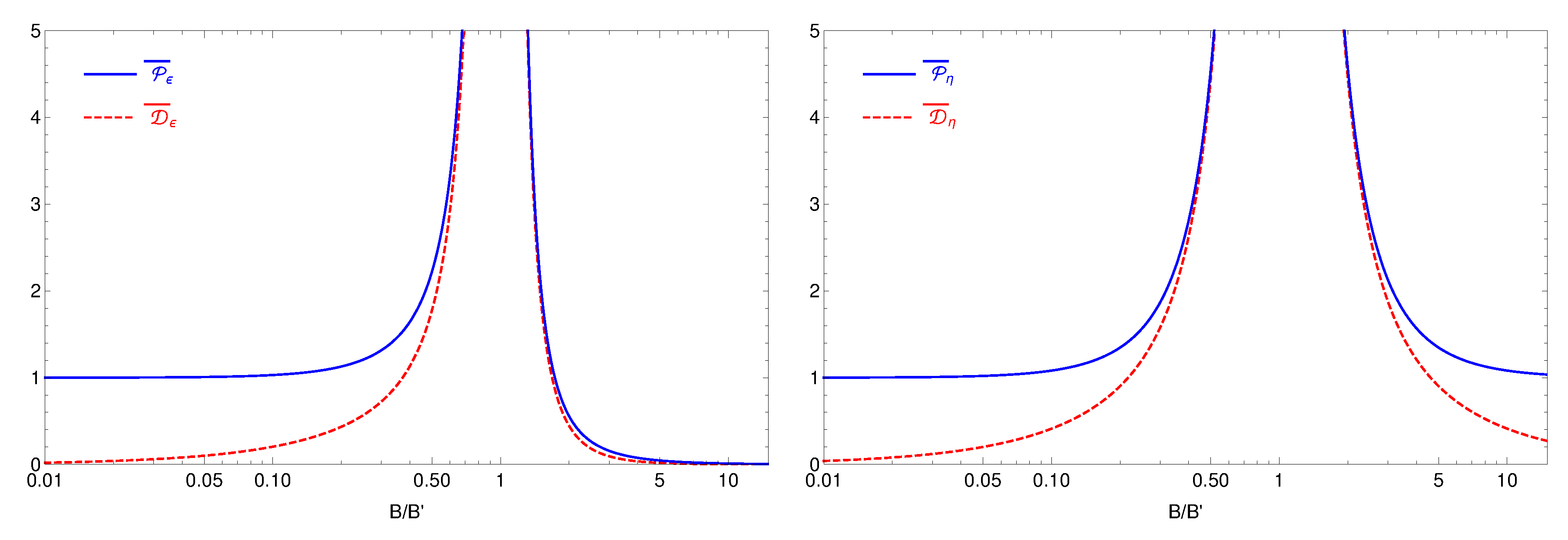
Thus, if , the probability of oscillation in vanishing magnetic field can be small, and it should be modified in larger magnetic fields. In particular, it can be resonantly enhanced when the applied magnetic field has the values comparable to . From Equations (10) and (15) we obtain the modification factor simply as a function of :
In principle, the scenarios of mass mixing and nTTM (in the case of + parity) can be distinguished by the shape of the oscillation probability in the neighbourhoods of the resonance (see Figure 1), which can be studied by scanning over the magnetic field values. As for the case of − parity, there is no resonant behaviour, the averaged probabilities are practically independent of B and thus, in this case the nTTM effects will be more difficult to distinguish. As for + parity case, the effect is substantial only when while in both limits and we have . (Very close to the resonance the probability will depend on the magnitude of magnetic field B and its direction also for − parity case.) Thus, for large magnetic fields probability will be constant independent on the parity sign as also can be seen directly from Equation (13).
On the other hand, assuming that , instead of applying non-zero magnetic field, one can introduce some matter potential for the ordinary component. In this case, taking , the Hamiltonians (5) should be changed to the form:
where now signs and indicate the neutron spin parallel/antiparallel respective to the mirror magnetic field direction . Correspondingly the oscillation probabilities (6) read:
Thus, at the resonance , the probability is resonantly enhanced to maximal value:
while for the same occurs for . Hence, by introducing some gas with positive or negative potential one could achieve a resonance amplification of conversion probability for one polarization, for both parities.
Let us consider e.g., the case of cold neutrons propagating in air or in another gas described by the positive Fermi quasi-potential [66]. At the same time, the density of this gas can be low enough to neglect the incoherent scattering at a finite angles and the absorption of neutrons. e.g., for air at normal temperature and pressure (NTP) this Fermi potential is neV. The probability of elastic scattering and absorption for cold neutrons in air at the NTP is ≈0.05 per meter of path. It is low enough to consider few meters of cold neutron beam propagation in air. In this way, if the polarization dependent losses will be observed, they can test the nTTM-induced conversions if the mirror magnetic field at the Earth is up to few Gauss.
3. Experimental Limits from Direct Searches with UCN
The experiments with the UCN traps such as [49,50,51,52,53,54] were performed for direct search of transition under the hypothesis of non-zero mass mixing . The above experiments study the dependence of the loss rate of the neutrons stored in the UCN traps on the strength and direction of the applied magnetic field . Under the assumption of possible presence of mirror magnetic field at the Earth, their results can be interpreted as upper limits on (or lower limits on oscillation time ) as a function of mirror field . Below, we shall use the results of these experiments for obtaining the similar limits on transitional moment . In this section we consider more interesting case corresponding to parity leaving the more simple case of negative parity, particularly in the resonant region, for discussion elsewhere.
The experimental strategy described e.g., in Ref. [54] is the following. In the absence of transitions, the number of neutrons surviving after effective storage time inside a UCN trap should not depend on , given that the usual UCN losses, such as neutron decay, wall absorption, or up-scattering, are magnetic field independent according to standard physics. But, when we consider oscillations, during the motion between two consecutive wall collisions the neutron can transform into a sterile state , and so per each collision it has a certain probability to escape from the trap. Therefore the number of survived neutrons in the UCN trap with applied magnetic field after a time is given by , where is the amount of UCN that would have survived in the absence of oscillation, is the average probability of conversion between the wall scatterings given in Equation (14) and is the mean number of wall scatterings for the neutrons survived after the time . The oscillation probability depends on strengths B and of magnetic fields and the angle between their directions, . If the magnetic field direction is inverted, , i.e., , we have . Then one can define the “directional” asymmetry between and as
where is the difference between the respective average oscillation probabilities which is proportional to and the expression of is given in Equation (15). The common factor cancels in the neutron count ratios, and directly traces the difference of the average oscillation probabilities in magnetic fields of the opposite directions, and .
One can also compare the average between those two counts: with the counts acquired under zero magnetic field. We then obtain:
where is the average of the oscillation probabilities between two opposite directions, see Equation (15). Thus, the value measuring the difference between the average probabilities at zero and non-zero magnetic fields should not depend on the magnetic field orientation but only on its modulus .
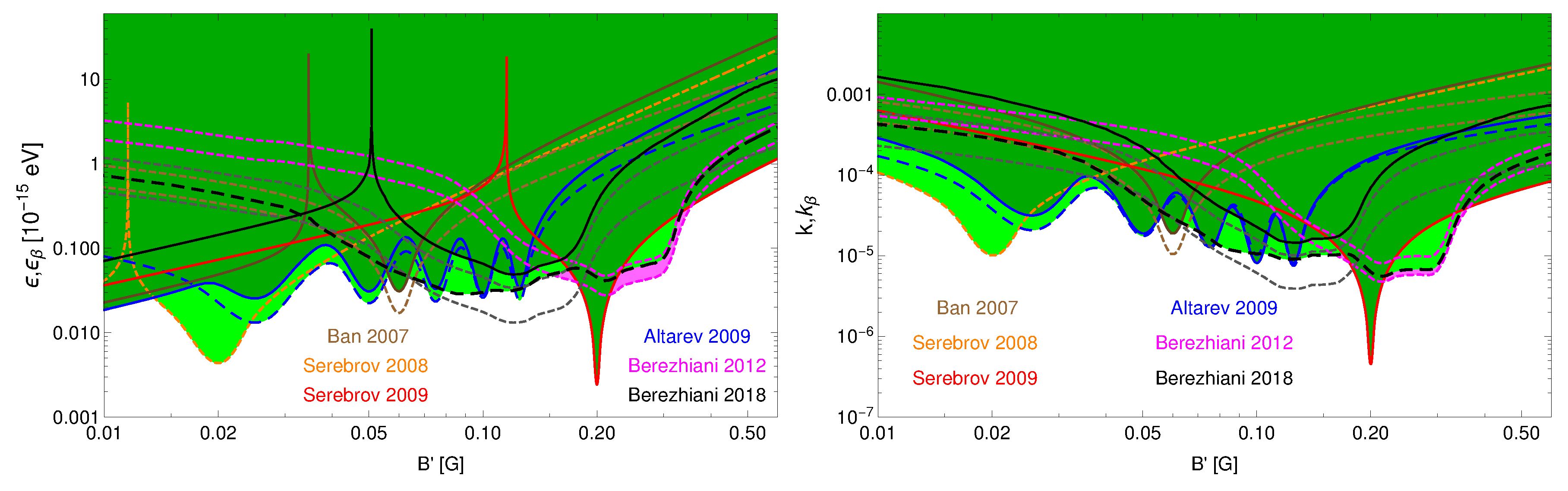
The current experimental situation in the case of mass mixing is summarised in Ref. [54]. These experiments, by measuring for different values of B, in fact determine the mass mixing parameter while via measuring they determine the combination , i.e., the mass mixing corrected by the unknown angle between the ordinary magnetic field and background mirror field . Namely, the results of all dedicated experiments [49,50,51,52,53,54] were used to set lower limits on the oscillation time and the combined value as a function of mirror magnetic field , see Figure 7 of Ref. [54] (in the limit , the upper limit corresponds to s at 90 % C.L. [50]). For convenience, in this paper (see left panel of Figure 2) we show the same limits directly in terms of physical parameters and as upper limits. (Clearly, in our generic context, these limits correspond to the case without nTTM contribution, i.e., .)
The data of the same measurements can be used for setting the upper limits on assuming in turn that mass mixing is vanishing and conversion occurs solely due to nTTM effects. In the right panel of Figure 2 we show upper limits on and in the case of . We used the same Monte Carlo code developed in [67] and used in [54] to calculate the average oscillation probability for the UCN inside the trap in non-homogeneous magnetic field but using the probabilities instead of . This will give us differences between the shapes of the exclusion regions for mass mixing and nTTM cases which can be observed by comparing the left and right panels of Figure 2. The magenta shaded areas in Figure 2 correspond to parameter regions relevant for more than deviation from null hypothesis in the measured asymmetry [55] which still is not excluded by the present experimental limits. Let us remind that this anomaly, as the variation of between the numbers of the survived UCN stored under the vertical magnetic field G directed up and down, was obtained in Ref. [55] via re-analysis of the experimental data of Ref. [51]. This asymmetry can been interpreted as an effect of oscillation in the presence of a mirror magnetic field on the order of 0.1 G at the Earth [54,55].
In this section we have not considered the effects of magnetic field gradients to be introduced in the following Section 4 for the estimates of possible magnitude of nTMM. In UCN experiments [49,50,51,52,53,54] certain attempts were made to maintain the uniformity of magnetic fields, so the effects of collapse of system in the trap volume between the wall collisions due to gradients might be not very significant besides the the fact that detailed field maps for most of these experiments are also not available. Thus, the limits shown on the right panel in Figure 2 should be considered as orientative upper limits for obtained in the assumption of the presence of mirror magnetic field .
4. System in Non-uniform Magnetic Field
If at the system were in vacuum and in a constant magnetic field (), then for initial condition at , the kinetic energies are the same, as it is assumed in Equation (3). The system will oscillate in time between two states n and which interact with ordinary matter differently. Two orthogonal eigenstates of the oscillating () system are formed corresponding to the different total energy eigenvalues. Namely, the Hamiltonian eigenstate has interaction properties close to that of the ordinary neutron (n) and the state close to that of the mirror neutron () once the mixing angle arising due to non-diagonal terms in Hamiltonian is small. In the medium is uniform and also constant in time, the eigenstates and do not oscillate between each other but just propagate independently. Let us remind however that in non-uniform medium the angle is position dependent and thus the notion of the Hamiltonian eigenstates has only a local significance. However if the evolution of the system is adiabatic, then the Hamiltonian eigenstates adiabatically evolve from one position to another.
Let us assume that at the system enters a region of non-uniform magnetic field which is a function of coordinates and has non-zero gradients. The gradient of potential energy from a semi-classical point of view generates a force. In some UCN experiments, e.g., in the UCN experiment with magnetic Hallbach array [68], this force can exceed the Earth gravitational attraction force and cause vertical bouncing of neutrons (of a certain polarization) from the surface with an arranged strong magnetic field gradient. By virtue of the Mirror Model this gradient force mainly acts on the “almost" neutron component of the system but very weakly on the “almost" mirror component , while the gravity is the same for both components and . A similar situation occurs in the collision of neutrons with the wall in gravitational UCN traps, where the gradient is due to the Fermi potential of the trap walls. A positive Fermi potential of the wall material will repulse neutrons with kinetic energy smaller than at the characteristic distance of the neutron wave packet, ∼ for typical neV. In this way, the gradient of potential in the interaction with wall can be estimated as ∼1 eV/m. In the UCN experiment [68] the gradient of the magnetic field is ∼1 T/cm near the bouncing surface that corresponds to the gradient of potential energy ∼ eV/m.
Integrated over time , this force provides a relative momentum between the two components. If it exceeds the width of the neutron wave packet , then that will lead to the “separation of components” or to decoherent collapse of system into either or states. If this force would be exerted only for time and then reduced to zero, then finite relative momentum will continue in time the separation of the components. The same conclusion can be formulated in a language more appropriate for quantum mechanics as a potential energy variation different for the two components of wave function in non-uniform magnetic field.
At some point the two components will be “pulled away” by gradient, and the entanglement of system moving in the non-uniform magnetic field will be broken. If “measured” at this moment the system will be found with probability P in the pure state of “mirror neutron” or with probability in the state of “neutron” . If not “measured,” each of the states will be subject to further oscillation with the reset of initial conditions at the time of “separation.”
The situation is similar in UCN traps with the material walls where entanglement will be broken with n component being reflected or absorbed by the wall with the probability and component escaping from the UCN trap through the wall with a small probability P.
More generally, the motion of the oscillating system in the slowly (adiabatically) changing magnetic field can lead either to a change of the kinetic energy of the components of wavefunction and/or to their spin rotation. Both these effects can result in decoherence of the system. The decoherence problem expectedly can be properly treated by modern methods using the density matrix formalism [69,70]. One can consider master equation of the evolution of density matrix of system in the environment of the external potential , different for two components of the system (four components when spins are included). These techniques are not yet sufficiently developed and tested in respect to particle oscillations and therefore we will refrain from the construction and solution of the density matrix evolution equation. Instead we try to consider the decoherence problem qualitatively. For these qualitative arguments we will ignore the spin rotation in a non-uniform magnetic field and will consider one-dimensional motion in a field with a gradient. Let us first assume a hypothetical simple case of a constant gradient of the magnetic field along the direction of the motion. The magnitude of B is linearly increasing with the distance x, but the direction of vector remains practically the same. For a neutron with a certain polarization propagating along axis x from the initial condition and for the observation time , the kinetic energy width of the wave packet of the system is:
For a path , passed by the neutron for the observation time , the change of potential energy produced by the magnetic field gradient is . If is much smaller than :
then the system will remain entangled.
For sufficiently large , the entanglement of the system will be broken. T his means that the system will collapse to pure states of either or n with probabilities P and correspondingly. Assuming that the velocity will not change significantly by magnetic gradient for the time (say, for the time of flight between two wall collisions in a UCN gravitational trap), then the gradient that should lead to the decoherence collapse of the system can be estimated in a following way:
Thus, for the entangled evolution of the system e.g., with velocity m/s in a UCN gravitational trap with a flight time s between wall collisions, the magnetic field gradient should be mG/m. Larger gradients can cause the collapse of the wavefunction at an earlier time and can cause the transformation of n to to occur in the volume of the trap rather than in collisions with the trap walls. Thus, the effect of a non-uniform magnetic field might result in the transformation in the trap volume with the same result as that which would be expected in collisions of the entangled system with the trap walls.
In the UCN gravitational trap experiments measuring the neutron lifetime the Earth magnetic field G is usually considered as a non-essential factor. The number of wall collisions is experimentally extrapolated to the “zero number of collisions,” e.g., in [71,72,73]. A magnetic field non-uniformity can produce a similar disappearance effect in the volume of UCN gravitational traps, but this effect is not removable by extrapolation to the zero number of wall collisions. Unfortunately, the UCN gravitational trap experiments do not use magnetic shielding of the trap, and the actual maps of magnetic fields in these experiments are unknown. For getting some idea of the possible non-uniformity of the Earth magnetic field in such conditions, we have measured some vertical gradients as high as 75 mG/m in an arbitrary general-purpose laboratory room of a typical university building. Therefore, we can advocate that the contribution of nTMM (that outside the resonance does not depend on the magnitude of the magnetic field) to transformation could be also essential as a source of the neutron loses.
In the proposed cold-neutron-beam disappearance/regeneration experiments [60,61], with average neutron velocity m/s and flight path e.g., 16 m, for the entangled evolution of the oscillating system the gradients ≪ mG/m would be required. Larger gradients can shorten the path of entangled evolution and effectively will lead to multiple shorter-in-time collapses which will increase the production of states, since the probability in the fields larger than few mG and far from resonance due to nTMM will remain constant .
5. Possible Magnitude of Neutron TMM
It is a well known problem in UCN gravitational trap experiments that the measured wall losses are larger than these predicted from theoretical models using known scattering lengths of materials (see discussion in Refs. [74,75] and references therein). Lowering the temperature of the trap walls, although reducing the loss coefficient (per single collision), does not resolve the discrepancy between experiment and theoretical calculations. Only in one of a few experiments using fomblin-oil coated trap [73] the measured () and expected () loss factors per wall collision were in good agreement. (In all other experiments the measured losses were significantly exceeding the theoretical predictions.) Hence, one can speculate that losses at least at the level of per collision can be due to the losses in the trap volume caused by the neutron TMM in the non-uniform environmental magnetic field. The local Earth magnetic field in these experiments can be affected by magnetic constructional materials, platforms, etc., as well as by metal reinforced concrete walls of the industrial buildings. Let us assume that in a typical trap of the size ∼0.3 m the magnetic field uniformity is <5% from wall to wall such that the moving neutron can see a constant gradient of about 75 mG/m. We are not considering the effect of neutron spin rotation due to possible change of the direction of the magnetic field—this might result in additional decoherence effects that are not discussed here. For a typical UCN velocity 3 m/s, and assuming that the velocity will not essentially be changed by the gradient during the flight from wall to wall, from Equation (25) we can find that the typical time for collapse to occur will be ∼ s. Thus, we can estimate that ∼5 volume collapse events will occur per one collision with the trap wall. Attributing this totally to the neutron TMM transformations with constant probability , we can estimate that losses per collision of correspond to a neutron TMM of
In the neutron lifetime measurement with large UCN gravitational trap [72], assuming the same magnetic field gradients, the number of decoherence events per second occurring in the volume of the storage trap can be estimated as ∼50 s. With the probability of transformation per event as , this can generate a neutron disappearance rate that can explain the difference [76] between the result [72] of the UCN disappearance lifetime experiment and the result of the beam appearance measurement [77]. The required value of nTMM in this case can be estimated again as (26).
If magnetic field gradients in the gravitational trap are higher than we have assumed, then the magnitude of neutron TMM required to produce mentioned disappearance rate can be lower than in (26). Also, if is present it might increase the conversion probability thus reducing our estimate of in (26). Would the UCN lifetime experiment with gravitational trap be magnetically shielded with residual field magnitude mG (that means assuming that both B and are vanishing) then effect due to nTMM will vanish and measured lifetime might be affected only by a smaller effect of oscillations due to mixing mass as was discussed earlier.
In experiments with “UCN magnetic field trap” [68,78], where neutrons are repulsed from the strong gradient of the magnetic field, the number of decoherence events can be greatly increased. For a rough estimate we have attempted to reproduce in a simplified one-dimensional way the vertical bouncing of UCN in the magnetic field with a strong gradient described in the papers [68] up to the height of 50 cm and obtained with Equation (25) approximately 3500 decoherence events per a second of the neutron motion. Thus, to produce a UCN disappearance rate ∼ per second in experiment [68], using constant conversion probability one can estimate the magnitude of nTMM:
Simulations for neutron propagation in the trap with more details of magnetic field configuration (not available to us) will likely affect this estimate. Also, the potential reason for disappearance in [68] can be a change of the spin precession phase due to the presence of oscillations [2] that can lead to unexpected depolarization effect in the magnetic trap.
We also can get another nTMM estimate from the different interpretation of the limit on obtained in [51] at and under assumption that . We will assume for this result instead that mirror magnetic field is present (although unknown) with magnitude larger than few mG and thus the measured limit on disappearance probability in [51] should be taken as a limit determined by the magnitude of probability due to nTMM. From this we can obtain the following estimate:
We can conclude this section by noting that these estimates, although very rough, are suggesting the order of magnitude of the nTMM that doesn’t contradict the existing experimental observations and might be the parameter of the mechanism responsible for the neutron disappearance in the UCN trap lifetime experiments, such as [68,72,78] and others. Such range of possible magnitudes for is also allowed by the limits obtained from the direct search discussed in Section 3.
6. How nTMM can be Measured
Beyond the results obtained in direct searches with UCN [49,50,51,52,53,54,55] and summarized in [54] the possible new searches with cold neutrons, described in [60,61], might bring more evidence whether transformation exists. These new proposed measurements are based on the detection of cold neutrons in intense beam after coming through the “region A” of controlled uniform magnetic field (in disappearance mode) or on total absorption of the cold neutron beam after passing through the “region A”, allowing only produced mirror neutron to pass through an absorber and then regenerating them back to the detectable neutrons in the second “region B” with similar controlled uniform magnetic field (regeneration mode). Variation of the magnitude of uniform magnetic field B in the range 0 to 0.5 G by small-steps scan (also with possible variation of direction of vector ) can reveal the resonance in the n-counting rates corresponding to with magnitude and width related to mass mixing parameter in Equation (4). The presence of nTMM can enhance the resonance magnitude or, as follows from Equation (15), can offer an alternative interpretation of the effect (if observed or excluded) in terms of magnitude of nTMM.
We would like to discuss here other two new methods that can be used for the detection of nTMM effect in the magnetic fields stronger than the Earth magnetic field.
The first method is a variation of the regeneration method where “region A” and “region B” mentioned above, instead of uniform magnetic field, are implementing strongly non-uniform magnetic field. Since nTMM transition probability remains constant in any sufficiently large magnetic field, strong gradients of the field can generate large number of decoherent collapses of system into either n, or with a small probability to -states; the latter will lead to enreachment of in the “region A.” The absorber between “region A” and “region B” will remove all not-transformed neutrons from the beam allowing only the to pass through the absorber. Strong gradients of the magnetic field in the “region B” will similarly enhance the transformation of back to detectable n, the latter can be counted above the natural background e.g., by the He detector.
Strong magnetic field gradients in “region A” and “region B” can be implemented e.g., as a series of equally spaced coils around the neutron beam with alternating directions of constant current. Every coil will contribute opposite direction of magnetic field with zig-zag pattern and can provide practically constant strong gradient along the beam axis. Simple estimates show that the gradient ∼100 G/m can be maintained along the vacuum tube that is e.g., 15 m long. For the cold neutron beam with average velocity ∼800 m/s using Equation (25) we can estimate that the number of decoherent collapses in such “region A”- or “region B”- devices will be around 500.
The use of superconducting solenoidal magnet with a borehole along the beam axis and with maximum magnetic field of ∼10 T will be a more compact approach for reaching high gradients. The total length of the magnet can be of the order of 1 m. The magnet front field ramping-up side can serve as a “region A” and back side with ramping-down field as a “region B,” each with a decoherence collapse factor ∼700. A beam absorber should be installed in the middle of the magnet, thus transforming it into a regeneration device.
With cold neutron beams available e.g., at ILL and at HFIR/ORNL reactors, or at SNS/ORNL, or at the future ESS spallation neutron source [79], where cold beam intensities are in the range – n/s, the effect of nTMM in the whole range of – can be explored in rather short and not expensive experiments [80].
The second method is based on the idea of compensation of Fermi quasi-potential of the gas media with a constant uniform magnetic field as discussed in the Section 2 of this paper with oscillation probability given by Equations (6) and (20). In Equation (6) both parameters of the resonance and are known and can be adjusted to compensate each other. Then, close to the resonance the probability of quasi-free oscillation can coherently grow as square of neutrons propagation time through the gas, e.g., through the air at NTP. This will work, according to Equation (6), only for one of neutron polarizations. Regeneration scheme can be used here again with “region A” and “region B” represented by the air-filled tubes of length e.g., m in the solenoidal constant uniform field of B∼10 G. Effects of the beam scattering and absorption in the gas will reduce the rate of regenerated neutrons by ≈20%. Probability of regeneration observation provided by this second method can be an order of magnitude higher than for the first method discussed above. If the resonance will be observed for the values different from anticipated zero, that will indicate the presence of either mirror magnetic field or small mirror Fermi-potential . In this case, the same two-tubes layout can be used foe regeneration search with the magnetic field B shielded below a ∼mG and the gas pressure in the tubes, i.e., parameter varied in order to find the resonance condition described by Equation (20) corresponding to the unknown mirror magnetic field . The second method can be further optimized for the use with a beam of collimated UCN propagating in the gas with low absorption. In this case, due to slow UCN velocities the probability for transformation potentially can grow approaching the maximum value.
7. Conclusions
Generally speaking, in this paper we discussed the possible environmental effects on the oscillating quantum system which environment can be related to dark matter. The paradigm of the neutron–mirror neutron transition [1] should naturally comprise additional effects that are inherent for mirror matter which essentially is a self-interacting atomic dark matter. This sort of dark matter, composed dominantly by lighter mirror nuclei as hydrogen and helium, is not easily accessible in direct dark matter search (see however Refs. [81,82]). But its collective environmental effects could have an interesting consequences for the fundamental particle properties and influence the values of the physical quantities such as particle lifetimes, spin precession frequencies, rates of baryon violating processes, etc. which effects are not yet adequately explored in the high precision particle physics experiments.
For the neutron–mirror neutron transitions which can be caused by the mass mixing and/or by transition magnetic (or electric) dipole moment between n and states, these environmental effects can be related to the existence of mirror magnetic fields on Earth [2], the possible accumulation of mirror matter in the solar system and inside the Earth which could also form the mirror atmosphere of the latter [31], and possibly other more exotic effects as long range fifth-forces [38,39] or gravity forces in bigravity theories [40,41], which can differently act on ordinary and mirror matter components. In difference from the ordinary matter environment which can be controlled (the gas can be pumped out for reaching a good vacuum and the magnetic field can be screened), environment of dark matter cannot be altered in experiments. Nevertheless, these effects can be probed experimentally.
The existing difference between the neutron lifetime measurements by the beam (appearance) experiments [77] and the UCN trap (disappearance) experiments [68,71,72,73,78] can be explained by conversions due to small transition magnetic moment. The magnitudes of nTMM extracted from the difference in neutron lifetime results can be measured in rather simple experiments, such as one proposed in [61] for the GP-SANS beamline at HFIR. If the mirror magnetic field with non-zero value is present, the experimental strategy with controlled uniform magnetic field B can be pursued, as described in the papers [60,61]. This would allow the detection of the process and could also reveal the environmental effects of mirror matter e.g. by determining the magnitude and the direction of mirror magnetic field. This might be a venue for observation of new effects which are usually ignored in experiments.
Author Contributions
Conceptualization, Z.B. and Y.K.; investigation: Z.B., R.B., Y.K. and L.V; software, R.B. and L.V.; formal analysis, R.B. and L.V.; writing—original draft preparation, Z.B. and Y.K.; writing—review and editing, Z.B., R.B., Y.K. and L.V.; contributions of all authors were of essential importance at all stages of the work.
Funding
The work of Z.B. was supported in part by the triennial research grant No. 2017X7X85K “The Dark Universe: Synergic Multimessenger Approach” under the program PRIN 2017 funded by the Ministero dell’Istruzione, Università e della Ricerca (MIUR) of Italy, and in part by triennial research grant DI-18-335/New Theoretical Models for Dark Matter Exploration funded by Shota Rustaveli National Science Foundation (SRNSF) of Georgia,. The work of Y.K. was partially supported by US DOE Grant DE-SC0014558. The work of L.V. was supported by the NSF Graduate Research Fellowship under Grant No. DGE-1746045.
Acknowledgments
We would like to thank Josh Barrow, Leah Broussard, Sergey Ovchinnikov, Yuri Pokotilovski, Anatoly Serebrov, George Siopsis and Arkady Vainshtein for useful discussions. We would like to thank also reviewers of this work for a careful reading of the manuscript and constructive suggestions. Z.B. and Y.K. acknowledge the hospitality provided by the Institute for Nuclear Theory, University of Washington, Seattle, where in October 2017 this work was initiated during the Workshop INT-17-69W “Neutron Oscillations: Appearance, Disappearance, and Baryogenesis.”
Conflicts of Interest
The authors declare no conflict of interest.
References
- Berezhiani, Z.; Bento, L. Neutron–mirror neutron oscillations: How fast might they be? Phys. Rev. Lett. 2006, 96, 081801. [Google Scholar] [CrossRef] [PubMed]
- Berezhiani, Z. More about neutron–Mirror neutron oscillation. Eur. Phys. J. C 2009, 64, 421. [Google Scholar] [CrossRef]
- Berezhiani, Z. Mirror world and its cosmological consequences. Int. J. Mod. Phys. A 2004, 19, 3775. [Google Scholar] [CrossRef]
- Berezhiani, Z. Through the Looking-glass: Alice’s Adventures in Mirror World. In From Fields to Strings: Circumnavigating Theoretical Physics; Shifman, M., Vainshtein, A., Wheater, J., Eds.; World Scientific: Singapore, 2005; Volume 3, pp. 2147–2195. [Google Scholar]
- Berezhiani, Z. Unified picture of ordinary and dark matter genesis. Eur. Phys. J. Spec. Top. 2008, 163, 271. [Google Scholar] [CrossRef]
- Lee, T.D.; Yang, C.N. Question of Parity Conservation in Weak Interactions. Phys. Rev. 1956, 104, 254. [Google Scholar] [CrossRef]
- Kobzarev, I.Y.; Okun, L.B.; Pomeranchuk, I.Y. On the possibility of experimental observation of mirror particles. Sov. J. Nucl. Phys. 1966, 3, 837. (Yad. Fiz. 1966, 3, 1154. (In Russian)) [Google Scholar]
- Blinnikov, S.I.; Khlopov, M.Y. On Possible Effects Of ‘mirror’ Particles. Sov. J. Nucl. Phys. 1982, 36, 472. (Yad. Fiz. 1982, 36, 809. (In Russian)) [Google Scholar]
- Khlopov, M.Y.; Beskin, G.M.; Bochkarev, N.E.; Pustylnik, L.A.; Pustylnik, S.A. Observational Physics of Mirror World. Sov. Astron. 1991, 35, 21. (Astron. Zh. 1991, 68, 42. (In Russian)) [Google Scholar]
- Foot, R.; Lew, H.; Volkas, R.R. A Model with fundamental improper space-time symmetries. Phys. Lett. B 1991, 272, 67. [Google Scholar] [CrossRef]
- Okun, L.B. Mirror particles and mirror matter: 50 years of speculations and search. Phys. Usp. 2007, 50, 380. [Google Scholar] [CrossRef]
- Holdom, B. Two U(1)’s and Epsilon Charge Shifts. Phys. Lett. 1986, 166B, 196. [Google Scholar] [CrossRef]
- Glashow, S.L. Positronium Versus the Mirror Universe. Phys. Lett. 1986, 167B, 35. [Google Scholar] [CrossRef]
- Carlson, E.D.; Glashow, S.L. Nucleosynthesis Versus the Mirror Universe. Phys. Lett. B 1987, 193, 168. [Google Scholar] [CrossRef]
- Gninenko, S.N. Limit on ’disappearance’ of orthopositronium in vacuum. Phys. Lett. B 1994, 326, 317. [Google Scholar] [CrossRef]
- Berezhiani, Z.; Lepidi, A. Cosmological bounds on the ’millicharges’ of mirror particles. Phys. Lett. B 2009, 681, 276. [Google Scholar] [CrossRef]
- Raaijmakers, M.; Gerchow, L.; Radics, B.; Rubbia, A.; Vigo, C.; Crivelli, P. New bounds from positronium decays on massless mirror dark photons. arXiv 2019, arXiv:1905.09128. [Google Scholar]
- Akhmedov, E.K.; Berezhiani, Z.; Senjanovic, G. Planck scale physics and neutrino masses. Phys. Rev. Lett. 1992, 69, 3013. [Google Scholar] [CrossRef]
- Foot, R.; Lew, H.; Volkas, R.R. Possible consequences of parity conservation. Mod. Phys. Lett. A 1992, 7, 2567. [Google Scholar] [CrossRef]
- Foot, R.; Volkas, R.R. Neutrino physics and the mirror world: How exact parity symmetry explains the solar neutrino deficit, the atmospheric neutrino anomaly and the LSND experiment. Phys. Rev. D 1995, 52, 6595. [Google Scholar] [CrossRef]
- Berezhiani, Z.; Mohapatra, R.N. Reconciling present neutrino puzzles: Sterile neutrinos as mirror neutrinos. Phys. Rev. D 1995, 52, 6607. [Google Scholar] [CrossRef] [PubMed]
- Berezhiani, Z. Unified picture of the particle and sparticle masses in SUSY GUT. Phys. Lett. B 1998, 417, 287. [Google Scholar] [CrossRef]
- Berezhiani, Z.; Rossi, A. Flavor structure, flavor symmetry and supersymmetry. Nucl. Phys. Proc. Suppl. 2001, 101, 410. [Google Scholar] [CrossRef]
- Belfatto, B.; Berezhiani, Z. How light the lepton flavor changing gauge bosons can be. Eur. Phys. J. C 2019, 79, 202. [Google Scholar] [CrossRef]
- Berezhiani, Z.; Comelli, D.; Villante, F.L. The Early mirror universe: Inflation, baryogenesis, nucleosynthesis and dark matter. Phys. Lett. B 2001, 503, 362. [Google Scholar] [CrossRef]
- Bento, L.; Berezhiani, Z. Leptogenesis via collisions: The Lepton number leaking to the hidden sector. Phys. Rev. Lett. 2001, 87, 231304. [Google Scholar] [CrossRef] [PubMed]
- Bento, L.; Berezhiani, Z. Baryon asymmetry, dark matter and the hidden sector. Fortsch. Phys. 2002, 50, 489. [Google Scholar] [CrossRef]
- Ignatiev, A.Y.; Volkas, R.R. Mirror dark matter and large scale structure. Phys. Rev. D 2003, 68, 023518. [Google Scholar] [CrossRef] [Green Version]
- Berezhiani, Z.; Ciarcelluti, P.; Comelli, D.; Villante, F.L. Structure formation with mirror dark matter: CMB and LSS. Int. J. Mod. Phys. D 2005, 14, 107. [Google Scholar] [CrossRef]
- Berezhiani, Z.; Cassisi, S.; Ciarcelluti, P.; Pietrinferni, A. Evolutionary and structural properties of mirror star MACHOs. Astropart. Phys. 2006, 24, 495. [Google Scholar] [CrossRef]
- Berezhiani, Z. Anti-dark matter: A hidden face of mirror world. arXiv 2016, arXiv:1602.08599. [Google Scholar]
- Berezhiani, Z. Matter, dark matter, and antimatter in our Universe. Int. J. Mod. Phys. A 2018, 33, 1844034. [Google Scholar] [CrossRef]
- Kuzmin, V.A. CP violation and baryon asymmetry of the universe. JETP Lett. 1970, 12, 335. [Google Scholar]
- Mohapatra, R.N.; Marshak, R.E. Local B-L Symmetry of Electroweak Interactions, Majorana Neutrinos and Neutron Oscillations. Phys. Rev. Lett. 1980, 44, 1316. [Google Scholar] [CrossRef]
- Phillips, D.G., II. Neutron-Antineutron Oscillations: Theoretical Status and Experimental Prospects. Phys. Rept. 2016, 612, 1. [Google Scholar] [CrossRef]
- Babu, K.; Banerjee, S.; Baxter, D.V.; Berezhiani, Z.; Bergevin, M.; Bhattacharya, S.; Brice, S.; Burgess, T.W.; Castellanos, L.; Chattopadhyay, S.; et al. Neutron-Antineutron Oscillations: A Snowmass 2013 White Paper. arXiv 2013, arXiv:1310.8593. [Google Scholar]
- Berezhiani, Z. Neutron–antineutron oscillation and baryonic majoron: Low scale spontaneous baryon violation. Eur. Phys. J. C 2016, 76, 705. [Google Scholar] [CrossRef]
- Babu, K.S.; Mohapatra, R.N. Limiting Equivalence Principle Violation and Long-Range Baryonic Force from Neutron-Antineutron Oscillation. Phys. Rev. D 2016, 94, 054034. [Google Scholar] [CrossRef]
- Addazi, A.; Berezhiani, Z.; Kamyshkov, Y. Gauged B-L number and neutron–antineutron oscillation: Long-range forces mediated by baryophotons. Eur. Phys. J. C 2017, 77, 301. [Google Scholar] [CrossRef]
- Berezhiani, Z.; Pilo, L.; Rossi, N. Mirror Matter, Mirror Gravity and Galactic Rotational Curves. Eur. Phys. J. C 2010, 70, 305. [Google Scholar] [CrossRef]
- Berezhiani, Z.; Nesti, F.; Pilo, L.; Rossi, N. Gravity Modification with Yukawa-type Potential: Dark Matter and Mirror Gravity. JHEP 2009, 0907, 83. [Google Scholar] [CrossRef]
- Berezhiani, Z.; Comelli, D.; Nesti, F.; Pilo, L. Spontaneous Lorentz Breaking and Massive Gravity. Phys. Rev. Lett. 2007, 99, 131101. [Google Scholar] [CrossRef] [Green Version]
- Berezhiani, Z.G.; Dolgov, A.D.; Mohapatra, R.N. Asymmetric inflationary reheating and the nature of mirror universe. Phys. Lett. B 1996, 375, 26. [Google Scholar] [CrossRef]
- Berezhiani, Z.G. Astrophysical implications of the mirror world with broken mirror parity. Acta Phys. Polon. B 1996, 27, 1503. [Google Scholar]
- Mohapatra, R.N.; Nussinov, S. Constraints on mirror models of dark matter from observable neutron–mirror neutron oscillation. Phys. Lett. B 2018, 776, 22. [Google Scholar] [CrossRef]
- Berezhiani, Z. Neutron lifetime puzzle and neutron–mirror neutron oscillation. Eur. Phys. J. C 2019, 79, 484. [Google Scholar] [CrossRef]
- Baldo-Ceolin, M.; Benetti, P.; Bitter, T.; Bobisut, F.; Calligarich, E.; Dolfini, R.; Dubbers, D.; El-Muzeini, P.; Genoni, M.; Gibin, D.; et al. A New experimental limit on neutron - anti-neutron oscillations. Z. Phys. C 1994, 63, 409. [Google Scholar] [CrossRef]
- Abe, K. The Search for n-n¯ oscillation in Super-Kamiokande I. Phys. Rev. D 2015, 91, 072006. [Google Scholar] [CrossRef]
- Ban, G.; Bodek, K.; Daum, M.; Henneck, R.; Heule, S.; Kasprzak, M.; Khomutov, N.; Kirch, K.; Kistryn, S.; Knecht, A.; et al. A Direct experimental limit on neutron–mirror neutron oscillations. Phys. Rev. Lett. 2007, 99, 161603. [Google Scholar] [CrossRef]
- Serebrov, A.P.; Aleksandrov, E.B.; Dovator, N.A.; Dmitriev, S.P.; Fomin, A.K.; Geltenbort, P.; Kharitonov, A.G.; Krasnoschekova, I.A.; Lasakov, M.S.; Murashkin, A.N.; et al. Experimental search for neutron–mirror neutron oscillations using storage of ultracold neutrons. Phys. Lett. B 2008, 663, 181. [Google Scholar] [CrossRef]
- Serebrov, A.P.; Aleksandrov, E.B.; Dovator, N.A.; Dmitriev, S.P.; Fomin, A.K.; Geltenbort, P.; Kharitonov, A.G.; Krasnoschekova, I.A.; Lasakov, M.S.; Murashkin, A.N.; et al. Search for neutron mirror neutron oscillations in a laboratory experiment with ultracold neutrons. Nucl. Instrum. Meth. A 2009, 611, 137. [Google Scholar] [CrossRef]
- Bodek, K.; Kuźniak, M.; Zejma, J.; Burghoff, M.; Knappe-Grüneberg, S.; Sander-Thoemmes, T.; Schnabel, A.; Trahms, L.; Ban, G.; Lefort, T.; et al. Additional results from the dedicated search for neutron mirror neutron oscillations. Nucl. Instrum. Meth. A 2009, 611, 141. [Google Scholar] [CrossRef]
- Altarev, I.; Baker, C.A.; Ban, G.; Bodek, K.; Daum, M.; Fierlinger, P.; Geltenbort, P.; Green, K.; van Der Grinten, M.G.D.; Gutsmiedl, E.; et al. Neutron to Mirror Neutron Oscillations in the Presence of Mirror Magnetic Fields. Phys. Rev. D 2009, 80, 032003. [Google Scholar] [CrossRef]
- Berezhiani, Z.; Biondi, R.; Geltenbort, P.; Krasnoshchekova, I.A.; Varlamov, V.E.; Vassiljev, A.V.; Zherebtsov, O.M. New experimental limits on neutron - mirror neutron oscillations in the presence of mirror magnetic field. Eur. Phys. J. C 2018, 78, 717. [Google Scholar] [CrossRef]
- Berezhiani, Z.; Nesti, F. Magnetic anomaly in UCN trapping: Signal for neutron oscillations to parallel world? Eur. Phys. J. C 2012, 72, 1974. [Google Scholar] [CrossRef]
- Berezhiani, Z.; Dolgov, A.D.; Tkachev, I.I. Dark matter and generation of galactic magnetic fields. Eur. Phys. J. C 2013, 73, 2620. [Google Scholar] [CrossRef]
- Berezhiani, Z.; Bento, L. Fast neutron: Mirror neutron oscillation and ultra high energy cosmic rays. Phys. Lett. B 2006, 635, 253. [Google Scholar] [CrossRef]
- Berezhiani, Z.; Gazizov, A. Neutron Oscillations to Parallel World: Earlier End to the Cosmic Ray Spectrum? Eur. Phys. J. C 2012, 72, 2111. [Google Scholar] [CrossRef]
- Mohapatra, R.N.; Nasri, S.; Nussinov, S. Some implications of neutron mirror neutron oscillation. Phys. Lett. B 2005, 627, 124. [Google Scholar] [CrossRef]
- Berezhiani, Z.; Frost, M.; Kamyshkov, Y.; Rybolt, B.; Varriano, L. Neutron Disappearance and Regeneration from Mirror State. Phys. Rev. D 2017, 96, 035039. [Google Scholar] [CrossRef]
- Broussard, L.J.; Bailey, K.M.; Bailey, W.B.; Barrow, J.L.; Chance, B.; Crawford, C.; Crow, L.; DeBeer-Schmitt, L.; Fomin, N.; Frost, M.; et al. New Search for Mirror Neutrons at HFIR. arXiv 2017, arXiv:1710.00767. [Google Scholar]
- Tanabashi, M.; Hagiwara, K.; Hikasa, K.; Nakamura, K.; Sumino, Y.; Takahashi, F.; Tanaka, J.; Agashe, K.; Aielli, G.; Amsler, C.; et al. Review of Particle Physics. Phys. Rev. D 2018, 98, 030001. [Google Scholar] [CrossRef] [Green Version]
- Berezhiani, Z.; Vainshtein, A. Neutron–Antineutron Oscillations: Discrete Symmetries and Quark Operators. Phys. Lett. B 2019, 788, 58. [Google Scholar] [CrossRef]
- Berezhiani, Z.; Vainshtein, A. Neutron–antineutron oscillation and discrete symmetries. Int. J. Mod. Phys. A 2018, 33, 1844016. [Google Scholar] [CrossRef]
- Berezhiani, Z. Neutron lifetime and dark decay of the neutron and hydrogen. LHEP 2019, 118, 1. [Google Scholar] [CrossRef]
- Golub, R.; Richardson, D.; Lamoreaux, S.K. Ultra-Cold Neutrons; Adam Hilger: Bristol, UK, 1991. [Google Scholar]
- Biondi, R. Monte Carlo simulation for ultracold neutron experiments searching for neutron–mirror neutron oscillation. Int. J. Mod. Phys. A 2018, 33, 1850143. [Google Scholar] [CrossRef]
- Pattie, R.W.; Callahan, N.B.; Cude-Woods, C.; Adamek, E.R.; Broussard, L.J.; Clayton, S.M.; Currie, S.A.; Dees, E.B.; Ding, X.; Engel, E.M.; et al. Measurement of the neutron lifetime using a magneto-gravitational trap and in situ detection. Science 2018, 360, 627. [Google Scholar] [CrossRef]
- Lindblad, G. On the Generators of Quantum Dynamical Semigroups. Commun. Math. Phys. 1976, 48, 119. [Google Scholar] [CrossRef]
- Gorini, V.; Kossakowski, A.; Sudarshan, E.C.G. Completely Positive Dynamical Semigroups of N Level Systems. J. Math. Phys. 1976, 17, 821. [Google Scholar] [CrossRef]
- Serebrov, A.; Varlamov, V.; Kharitonov, A.; Fomin, A.; Pokotilovski, Y.; Geltenbort, P.; Butterworth, J.; Krasnoschekova, I.; Lasakov, M.; Tal’daev, R.; et al. Measurement of the neutron lifetime using a gravitational trap and a low-temperature Fomblin coating. Phys. Lett. B 2005, 605, 72. [Google Scholar] [CrossRef]
- Serebrov, A.P.; Kolomensky, E.A.; Fomin, A.K.; Krasnoschekova, I.A.; Vassiljev, A.V.; Prudnikov, D.M.; Shoka, I.V.; Chechkin, A.V.; Chaikovskiy, M.E.; Varlamov, V.E.; et al. Neutron lifetime measurements with the big gravitational trap for ultracold neutrons. JETP Lett. 2017, 106, 613. [Google Scholar] [CrossRef]
- Serebrov, A.P.; Varlamov, V.E.; Kharitonov, A.G.; Fomin, A.K.; Pokotilovski, Y.N.; Geltenbort, P.; Krasnoschekova, I.A.; Lasakov, M.S.; Taldaev, R.R.; Vassiljev, A.V.; et al. Neutron lifetime measurements using gravitationally trapped ultracold neutrons. Phys. Rev. C 2008, 78, 035505. [Google Scholar] [CrossRef] [Green Version]
- Goremychkin, E.A.; Pokotilovski, Y.N. Neutron lifetime and density of states of fluoropolymers at low temperatures. JETP Lett. 2017, 105, 548. [Google Scholar] [CrossRef]
- Goremychkin, E.A.; Pokotilovski, Y.N. Experimental density of states and the UCN loss coefficient of fluoropolymers at low temperatures. In Proceedings of the International Workshop Probing Fundamental Symmetries and Interactions with UCN, JGU Mainz, Germany, 11–15 April 2016. [Google Scholar]
- Pokotilovski, Y.N. On the experimental search for neutron → mirror neutron oscillations. Phys. Lett. B 2006, 639, 214. [Google Scholar] [CrossRef]
- Yue, A.T.; Dewey, M.S.; Gilliam, D.M.; Greene, G.L.; Laptev, A.B.; Nico, J.S.; Snow, W.M.; Wietfeldt, F.E. Improved Determination of the Neutron Lifetime. Phys. Rev. Lett. 2013, 111, 222501. [Google Scholar] [CrossRef] [Green Version]
- Ezhov, V.F.; Andreev, A.Z.; Ban, G.; Bazarov, B.A.; Geltenbort, P.; Glushkov, A.G.; Knyazkov, V.A.; Kovrizhnykh, N.A.; Krygin, G.B.; Naviliat-Cuncic, O.; et al. Measurement of the neutron lifetime with ultra-cold neutrons stored in a magneto-gravitational trap. JETP Lett. 2018, arXiv:1412.7434 [nucl-ex]. [Google Scholar]
- Peggs, S. ESS Technical Design Report. Available online: http://inspirehep.net/record/1704813/ (accessed on 15 Jul 2019).
- Nordita Workshop. Particle Physics with Neutrons at the ESS; Stockholm University: Stockholm, Sweden, 10–14 December 2018; Available online: http://agenda.albanova.se/conferenceTimeTable.py?confId=6570 (accessed on 10 August 2019).
- Cerulli, R.; Villar, P.; Cappella, F.; Bernabei, R.; Belli, P.; Incicchitti, A.; Addazi, A.; Berezhiani, Z. DAMA annual modulation and mirror Dark Matter. Eur. Phys. J. C 2017, 2017. 77, 83. [Google Scholar] [CrossRef]
- Addazi, A.; Berezhiani, Z.; Bernabei, R.; Belli, P.; Cappella, F.; Cerulli, R.; Incicchitti, A. DAMA annual modulation effect and asymmetric mirror matter. Eur. Phys. J. C 2015, 75, 400. [Google Scholar] [CrossRef]
Figure 1.
(blue) and (red) normalized over (left pane) vs. (blue) and (red) normalized over (right panel) as functions of the ratio , see Equations (17).
Figure 1.
(blue) and (red) normalized over (left pane) vs. (blue) and (red) normalized over (right panel) as functions of the ratio , see Equations (17).

Figure 2.
Upper limits for the oscillation parameters , assuming (left panel) and , assuming (right panel) as a function of the mirror magnetic field . The parameter areas excluded at 95 % C.L. by the experiments [49,50,51,52,53,54] for () are confined by solid curves of respective colors and are shaded in dark green, and for () are confined by dashed curves of respective colors and shaded by light green. Dashed pink curves confine the parameter area which can be relevant for anomaly in reported in Ref. [55], and its part still not excluded by other data is shaded in pink. Let us remark, that the exclusion areas are obtained by assuming that the magnitude of mirror field and/or its direction with respect to the laboratory site remained unchanged during several years of time lapse between experiments [49,50,51,52,53,54] which however might not be the case.

© 2019 by the authors. Licensee MDPI, Basel, Switzerland. This article is an open access article distributed under the terms and conditions of the Creative Commons Attribution (CC BY) license (http://creativecommons.org/licenses/by/4.0/).
Share and Cite
MDPI and ACS Style
Berezhiani, Z.; Biondi, R.; Kamyshkov, Y.; Varriano, L. On the Neutron Transition Magnetic Moment. Physics 2019, 1, 271-289. https://0-doi-org.brum.beds.ac.uk/10.3390/physics1020021
AMA Style
Berezhiani Z, Biondi R, Kamyshkov Y, Varriano L. On the Neutron Transition Magnetic Moment. Physics. 2019; 1(2):271-289. https://0-doi-org.brum.beds.ac.uk/10.3390/physics1020021
Chicago/Turabian StyleBerezhiani, Zurab, Riccardo Biondi, Yuri Kamyshkov, and Louis Varriano. 2019. "On the Neutron Transition Magnetic Moment" Physics 1, no. 2: 271-289. https://0-doi-org.brum.beds.ac.uk/10.3390/physics1020021