Dynamic Finite Element Modelling and Vibration Analysis of Prestressed Layered Bending–Torsion Coupled Beams

Abstract

Free vibration analysis of prestressed, homogenous, Fiber-Metal Laminated (FML) and composite beams subjected to axial force and end moment is revisited. Finite Element Method (FEM) and frequency-dependent Dynamic Finite Element (DFE) models are developed and presented. The frequency results are compared with those obtained from the conventional FEM (ANSYS, Canonsburg, PA, USA) as well as the Homogenization Method (HM). Unlike the FEM, the application of the DFE formulation leads to a nonlinear eigenvalue problem, which is solved to determine the system’s natural frequencies and modes. The governing differential equations of coupled flexural–torsional vibrations, resulting from the end moment, are developed using Euler–Bernoulli bending and St. Venant torsion beam theories and assuming linear harmonic motion and linearly elastic materials. Illustrative examples of prestressed layered, FML, and unidirectional composite beam configurations, exhibiting geometric bending-torsion coupling, are studied. The presented DFE and FEM results show excellent agreement with the homogenization method and ANSYS modeling results, with the DFE’s rates of convergence surpassing all. An investigation is also carried out to examine the effects of various combined axial loads and end moments on the stiffness and fundamental frequencies of the structure. An illustrative example, demonstrating the application of the presented methods to the buckling analysis of layered beams is also presented.

1. Introduction

Vibration is one of the main causes of structural failure, which makes it one of the most important and ongoing research fields in structural modelling and analysis. Multilayered structures, with their increasing applications in aerospace, mechanical and civil engineering, are subjected to different types of preloads based on their application. One of these prestress conditions is combined axial force and end moment which, for instance, happens where structural members are interconnected through an imperfect joint. Layered and laminated composite materials, e.g., Fiber-Metal Laminates (FMLs), are more prone to failure under these conditions due to their manufacturing nature. FML materials consist of layers of metal sheet and unidirectional fiber layers embedded in an adhesive system. Glare, an optimized FML with increasing applications in aircraft manufacturing, consists of alternating layers of aluminum and glass fiber prepreg layers.

The governing differential equations describing the motion for many beam configurations have been already developed and reported in the literatures. Neogy and Murthy [1] carried out one of the earliest studies around prestressed beams and found the fundamental frequency of an axially loaded column for two different boundary conditions of pinned-pinned and clamped-clamped. Prasad et al. [2] introduced a solution using Rayleigh-Ritz principles in an iterative form, and in comparison, with other approximate methods.

The bending-torsion coupled vibration of beams caused by cross-sectional geometry was first addressed by Timoshenko [3] and has been further studied by, among many other researchers, the second author (and his co-workers) to develop new solution methods, or to include diverse effects such as axial load (see, for example, [4,5]). Materially coupled vibrations of beams caused by different material couplings [6,7] have also been addressed and the governing differential equations describing the motion of various beam configurations have been developed [8,9]. Stability and vibrational analyses of beams subjected to axial preload and its effects on the beam stiffness and elasticity have also been conducted [10,11]. However, the vibration analysis of beams subjected to combined axial force and end moment is scarce [12,13,14].

Many analytical, semi-analytical and numerical methods have been developed to find solutions to the governing differential equations of motion. The Finite Element Method (FEM), as the most popular computational method in structural mechanics, has been extensively implemented by researchers (see, for example, [15,16,17]). Analytical solutions have also been formulated for the vibration analysis of various beam configurations [11,15] and Banerjee et al. [18] presented a Dynamic Stiffness Matrix (DSM) for coupled bending–torsion beam elements. Hashemi [19] introduced the frequency-dependent Dynamic Finite Element (DFE) method, a hybrid method bridging the gap between the conventional FEM and DSM methods. The DFE combines the accuracy of analytical methods with the versatility of numerical methods to conduct a vibration analysis of structural elements exhibiting coupled behaviours. The DFE formulation has since been further extended to vibration analysis of more complex beam configurations (see, for example [4,5,6,7]).

More recently, Ahmet Hasim [20] presented an isogeometric refined zigzag finite element (IGRZF) model that gives the opportunity to obtain the exact beam geometries directly from a computer aided design (CAD) software, Rhinoceros. The employed kinematics is based on the refined zigzag theory that makes the finite element independent from the number of layers considered. In this method, not only the element does not suffer from shear locking and geometric error, but it also does not need shear correction factors. The presented IGRZF approach is then used to analyze various sandwich beams. Later, Kefal et al. [21] extended this method to perform quasi-static structural analysis of sandwich and laminated composite beams with embedded delamination. An incomplete interaction, leading to interlayer slip, has also been considered and modeled. Foraboschi [22] introduced a 2D mathematical model for a two-layer beam, considering interlayer slip. Cas et al. [23] presented a derivation of a new mathematical model and its analytical solution for the analysis of geometrically and materially linear, 3D, two-layer, composite beams, with interlayer slips between the layers for the first time. In this study, it is assumed that there is no incomplete interaction between the layers.

Cortés and Sarría [24] presented a dynamic analysis of 3-Layer sandwich beams with thick viscoelastic damping core for FEM applications. They introduced a modified RKU model [25]. RKU model, originally proposed by Ross, Kerwin and Ungar [25] for the vibration modeling of viscoelastic laminate, is one of the first methods developed to find the flexural stiffness of sandwich beams and it is still commonly used in engineering applications because of its ease of computational implementation. Although RKU applies to simply supported beams it has been used for other types of boundary conditions as well. Besides other boundary conditions, Cortés and Sarría [24] used RKU for the dynamic analysis of cantilevered sandwich beams.

There are many studies on other aspects of the beam’s dynamics and stability. Mohri et al. [26] studied the vibration of buckled thin-walled beams with open sections. They dealt with small, superimposed vibrations of thin-walled elements with various open sections such as bisymmetric sections. They investigated vibration under two types of static pre-loadings: pure compression and lateral bending forces. A nonlinear model which accounts for nonlinear warping, bending-bending and torsion-bending couplings was used for the analysis. Franzoni et al. [27] proposed a numerical approach, based on a nonlinear finite element model and an experimental modal analysis procedure, to estimate the dynamic behavior of a typical aeronautical aluminum box-beam structure liable to buckling. Augello et al. [28] proposed an efficient Carrera Unified Formulation (CUF)-based method for the vibrations and buckling of thin-walled open cross-section beams, with complex geometries, under progressive compressive loads. A comprehensive study was also conducted in order to investigate the effects of compressive loads on the natural frequencies of the thin-walled beams. Namely, a numerical simulation of the Vibration Correlation Technique was provided. Finite Elements were built in the framework of the CUF, and the displacements of complex geometric shapes of the thin-walled beams were evaluated using low- to higher-order Taylor and Lagrange polynomials.

As mentioned earlier, the coupled free vibration analysis of homogeneous beams subjected to combined axial force and end moment has only been investigated in a few semi-analytical studies [12,13,14]. The geometrically coupled flexural–torsional vibration of homogeneous beams caused by combined prestress was recently revisited by the authors, using both FEM and DFE methods [29,30,31]. To the authors’ best knowledge, the geometrically coupled flexural–torsional vibration of layered beams, in the presence of combined axial load and end moment has not been reported in the open literature. In what follows, the coupled flexural–torsional vibration of axially-loaded layered beams, caused by the end moment is investigated and two formulations are presented.

The presented mathematical model is based on some simplifying assumptions, which lead to computational benefits for the presented methods. An equivalent single-layer formulation, similar to that presented in the RKU model and used by Cortés and Sarría [24], is exploited. The equivalent single-layer model is then discretized (along the beam length) using FEM [29,31] and DFE [30]. The application of the presented theory is demonstrated through the vibration analysis of illustrative prestressed layered beams. The presented layered FEM and DFE results show excellent agreement with homogenization method and ANSYS modeling results, with the DFE’s rates of convergence surpassing all. An investigation is also carried out to examine the effects of various combined axial loads and end moments on the stiffness and fundamental frequencies of the structure. An illustrative example, demonstrating the application of the presented methods to the buckling analysis of layered beams is also presented.

The structure of the paper is as follows: In Section 2, the concept of coupled, linear, undamped, free vibration of prestressed multi-layer beam, is presented followed by the expressions for the Galerkin-type integral form of the governing differential equations. Next, two layered beam conventional FEM (LBFEM) and Dynamic, frequency dependent (LBDFE) formulations are presented. In Section 3, the application of presented formulations to four cases of Steel-rubber-steel layered beam (Section 3.1), Cantilever Three-layered Fiber-Metal Laminated (FML) Beam (Section 3.2), and Cantilever Three-layered Laminated Composite Beam (Section 3.3), are presented. In Section 4, a discussion of the results obtained is provided followed by final conclusions that summarize the most important achievements of the article.

2. Materials and Methods

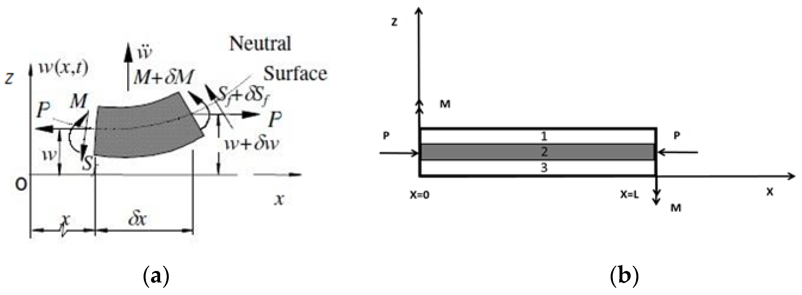
Consider a (three-)layered beam subjected to two equal and opposite end moments, M_zz, about z-axis and an axial load, P, loaded in the plane of greater bending rigidity, undergoing linear coupled torsion and lateral vibrations along the z-axis. Figure 1 depicts the schematic of the problem, where L, h and t stand for the beam’s length, width and height, respectively. As mentioned earlier, the presented mathematical model is based on an equivalent single-layer formulation, similar to that presented in the RKU model and used in [24]. The equivalent single-layer model is discretized (along the beam length) using FEM [29,31] and DFE [30]. The flexural and torsional rigidities of the equivalent single-layer beam are obtained by the addition of the individual contribution of each layer (calculated with respect to the beam neutral axis) [24,28]. It is assumed that the equivalent single-layer beam undergoes bending and torsional displacements and vibrates in a way like the original layered configuration, i.e., dynamically equivalent. One might put this in an overly simplistic way by saying all layers exhibit the same transverse displacement, slope, and torsional rotation. However, in reality this would violate interlayer lateral and axial displacements’ continuity and the use of a beam model accounting for 3D motion is preferable. Even so, the equivalent single-layer model in the vibration analysis of layered beams is commonly used [24,25].

For composite layers, the lamina theory and the method of homogenization are first used to find the equivalent physical properties of each layer, which are then used to obtain the equivalent single-layer beam model. Exploiting the classical lamination theory, a homogenized beam model is also developed and is used for the validation purposes. In this case, the apparent material properties (equivalent ρ, E, G, …) are used to treat the original layered beam as a simple beam. Consequently, only one set of (two coupled) equations of motion, with the homogenized parameters are solved. In contrast, the equivalent single-layer model uses equivalent flexural and torsional rigidities obtained and three sets of equations (six equations in total), combined as two, are solved.

Governing differential equations of motion is developed by defining an infinitesimal element using the following assumptions:

• The displacements are small.
• The stresses induced are within the limit of proportionality.
• The cross–section of the beam has two axes of symmetry.
• The cross–sectional dimensions of the beam are small compared to the span.
• The transverse cross–sections of the beam remain plane and normal to the neutral axis during bending, and
• The beam’s torsional rigidity (GJ) is assumed to be very large compared with its warping rigidity (EΓ), and ends are free to warp, i.e., state of uniform torsion.
• Damping is neglected.

Using the above-mentioned assumptions, it can be shown [12,26] that the governing differential equations for a prismatic, Euler–Bernoulli beam (EI = constant) subjected to constant axial force (P) and end moment (M_zz), and undergoing coupled flexural-torsional vibrations (caused by end moment), are as follows:

$$EI{w}^{⁗}+P{w}^{″}+M_{zz}{\theta }^{″}-\rho A\ddot{w}=0$$

(1)

$$GJ{\theta }^{″}+\frac{P{I}_P}{A}{\theta }^{″}+M_{zz}{w}^{″}-\rho I_P\ddot{\theta }=0$$

(2)

where ()′, stands for derivative with respect to x and (^•) denotes derivative with respect to t (time). As can be observed from Equations (1) and (2), the system is coupled by the end-moments, M_zz. The pre-stress effects of axial load and end moment are represented by the second and third terms in Equations (1) and (2). These coupling rigidities will result in a (coupling) stiffness matrix which represents the pre-stress effects on the beam’s rigidity.

Exploiting the simple harmonic motion assumption, displacements, w and θ, are written as:

$$w\left(x,t\right)=\hat{W}\mathit{sin}(\omega t),$$

(3)

$$\theta \left(x,t\right)=\widehat{\theta }\mathit{sin}(\omega t),$$

(4)

where ω denotes the frequency, $\widehat{W}$ and $\widehat{\theta }$ are the amplitudes of flexural and torsional displacements, respectively. Substituting Equations (3) and (4) into Equations (1) and (2) leads to:

$$EI{\widehat{W}}^{⁗}+P{\widehat{W}}^{″}+M_{zz}{\widehat{\theta }}^{″}-\rho A{\omega }^2\widehat{W}=0$$

(5)

$$GJ{\widehat{\theta }}^{″}+P{I}_P{\widehat{\theta }}^{″}+M_{zz}{\widehat{W}}^{″}-\rho I_{P}A{\omega }^2\widehat{\theta }=0$$

(6)

As, in this case, there are three layers with different materials, one will have three sets of equations, i.e., two for each layer and six equations in total, written as (I = 1, 2, 3):

$$EI{\widehat{W}}^{⁗}+P{\widehat{W}}^{″}+M_{zz}{\widehat{\theta }}^{″}-\rho A{\omega }^2\widehat{W}=0$$

(7)

$$G_i{J}_i{{\widehat{\theta }}_i}^{″}+P_i{I}_{P,i}{{\widehat{\theta }}_i}^{″}+M_{zz,i}{{\widehat{W}}_i}^{″}-{\rho }_i{I}_{P,i}{A}_i{\omega }^2{\widehat{\theta }}_i=0$$

(8)

where indices 1, 2 and 3 represent the properties of layer 1, layer 2 and layer 3, respectively. The second moment of inertia and polar moment of inertia for each layer is calculated about the neutral axis of the whole (beam) cross–section, and axial force and moment equilibrium equations are written as:

$$P=P_1+P_2+P_3, \mathrm{and} M_{zz}=M_{zz,1}+M_{zz,2}+M_{zz,3}$$

(9)

It is worth noting that Equations (7) and (8) can be readily extended to n-layer beam configurations (i.e., I = 1, 2, …, n). Assuming linearly elastic materials, an equivalent single-layer beam model [24,28] is developed, which vibrates in a similar way as the original layered configuration. The equivalent single-layer beam, governed by the pair of coupled Equations (7) and (8), undergoes bending displacement, $\widehat{W}$, and torsional displacement, θ. Simply put, the lateral and torsional displacements and slope of all layers are set equal (like ANSYS ‘constraint rigid link’ element [32]); i.e., ${\hat{W}}_1={\hat{W}}_2={\hat{W}}_3=\widehat{W}$ and ${\hat{\theta }}_1={\hat{\theta }}_2={\hat{\theta }}_3=\widehat{\theta }$. In other words, the summation of three bending equations describes the bending equation of the whole beam and the summation of three torsion equations describes the torsion equation of the equivalent single-layer beam, resulting in the following two through-the-thickness equations:

$$\begin{gathered} \left(E_1{I}_1+E_2{I}_2+E_3{I}_3\right){\widehat{W}}^{⁗}+\left(P_1+P_2+P_3\right){\widehat{W}}^{″}+\left(M_{zz,1}+M_{zz,2}+M_{zz,3}\right){\widehat{\theta }}^{″} \\ -\left({\rho }_1{A}_1+{\rho }_2{A}_2+{\rho }_3{A}_3\right){\omega }^2\widehat{W}=0, \end{gathered}$$

(10)

$$\begin{gathered} \left(G_1{J}_1+G_2{J}_2+G_3{J}_3\right){\widehat{\theta }}^{″}+\left(P_1{I}_{P,1}+P_2{I}_{P,2}+P_3{I}_{P,3}\right){\widehat{\theta }}^{″}+\left(M_{zz,1}+M_{zz,2}+M_{zz,3}\right){\widehat{W}}^{″} \\ -\left({\rho }_1{I}_{P,1}{A}_1+{\rho }_2{I}_{P,2}{A}_2+{\rho }_3{I}_{P,3}{A}_3\right){\omega }^2\widehat{\theta }=0, \end{gathered}$$

(11)

where the bending and torsional rigidities of all layers (E_iI_i, and G_iJ_i, i = 1, 2, 3, in this case.) are calculated with respect to the neutral axis of the overall cross–sectional area. In other words, as previously mentioned, the addition terms of flexural and torsional rigidities, (E₁I₁ + E₂I₂ + E₃I₃) and (G₁J₁ + G₂J₂ + G₃J₃), respectively, represent the corresponding rigidities for the equivalent single-layer beam model [24,28].

The Galerkin method of weighted residuals is employed to develop the integral form of the above equations, written as (note: from this point on, the hat sign has been omitted for simplicity):

$$\begin{gathered} {\overline{W}}_f={{\displaystyle \int }}_0^L\delta W(\left(E_1{I}_1+E_2{I}_2+E_3{I}_3\right)W^{⁗}+\left(P_1+P_2+P_3\right)W^{″}+\left(M_{zz,1}+M_{zz,2}+M_{zz,3}\right){\theta }^{″} \\ -\left({\rho }_1{A}_1+{\rho }_2{A}_2+{\rho }_3{A}_3\right){\omega }^{2}W)dx=0 \end{gathered}$$

(12)

$$\begin{gathered} {\overline{W}}_t={{\displaystyle \int }}_0^L\delta \theta (\left(G_1{J}_1+G_2{J}_2+G_3{J}_3\right){\theta }^{″}+\left(P_1{I}_{P,1}+P_2{I}_{P,2}+P_3{I}_{P,3}\right){\theta }^{″}+\left(M_{zz,1}+M_{zz,2}+M_{zz,3}\right)W^{″}- \\ \left({\rho }_1{I}_{P,1}{A}_1+{\rho }_2{I}_{P,2}{A}_2+{\rho }_3{I}_{P,3}{A}_3\right){\omega }^2\theta )dx=0 \end{gathered}$$

(13)

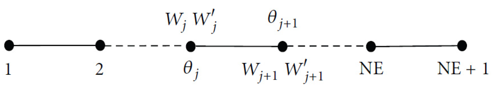
where δW and δθ (i.e., weighting functions) represent the transverse and torsional virtual displacements, respectively. Performing integration by parts on Equations (12) and (13) leads to the weak integral form of the governing equations, where the resulting boundary terms vanish irrespective of boundary conditions [33]. The beam is then discretized along its length (see Figure 2), leading to the following element integral equations:

$$\begin{gathered} {\overline{W}}_f^k={\int }_0^l(\left(E_1{I}_1+E_2{I}_2+E_3{I}_3\right)W^{″}\delta W^{″}+\left(P_1+P_2+P_3\right)W^{\prime }\delta W^{\prime }+ \\ \left(M_{zz,1}+M_{zz,2}+M_{zz,3}\right){\theta }^{\prime }\delta W^{\prime }-\left({\rho }_1{A}_1+{\rho }_2{A}_2+{\rho }_3{A}_3\right){\omega }^{2}W\delta W)dx \end{gathered}$$

(14)

$$\begin{gathered} {\overline{W}}_t^k={\int }_0^l(\left(G_1{J}_1+G_2{J}_2+G_3{J}_3\right){\theta }^{\prime }\delta {\theta }^{\prime }+\left(P_1{I}_{P,1}+P_2{I}_{P,2}+P_3{I}_{P,3}\right){\theta }^{\prime }\delta {\theta }^{\prime }+ \\ \left(M_{zz,1}+M_{zz,2}+M_{zz,3}\right)W^{\prime }\delta {\theta }^{\prime }-\left({\rho }_1{I}_{P,1}{A}_1+{\rho }_2{I}_{P,2}{A}_2+{\rho }_3{I}_{P,3}{A}_3\right){\omega }^2\theta \delta \theta )dx \end{gathered}$$

(15)

The above expressions (14) and (15), also satisfies the principle of virtual work ($\overline{W}={\overline{W}}_f+{\overline{W}}_t=0,$ with ${\overline{W}}_{EXT}=0$, for free vibrations), where:

$$\overline{W}={\overline{W}}_{INT}={\sum }_{K=1}^{No. of elements}{\overline{W}}^k={\sum }_{K=1}^{No. of elements}{\overline{W}}_f^k+{\overline{W}}_t^k$$

(16)

2.1. The Layered Beam Finite Element (LBFEM) Formulation

The layered beam FEM (LBFEM) formulation is attained by introducing linear and cubic Hermite polynomial interpolation functions to express the field and virtual variables (W, θ, δW and δθ), expressed in terms of nodal variables, subsequently introduced in expressions (14) and (15). This procedure leads to the LBFEM, with through-the-thickness mass, [m]^k, and stiffness, [k]^k, matrices written as:

[k]^k = [k]^k_flex + [k]^k_tor + [k]^k_coupling

(17)

where [k]^k_flex and [k]^k_tor are the element uncoupled flexural and torsional stiffness matrices, respectively, and [k]^k_Coupling is the element coupling stiffness matrix resulting from the end moment, M_zz. Furthermore, each of the [k]^k_flex and [k]^k_tor are written as:

[k]^k_flex = [k]^k_flex-Static + [k]^k_flex-Geo and [k]^k_tor = [k]^k_tor-Static + [k]^k_tor-Geo

(18)

where [k]^k_flex-Static and [k]^k_tor-Static are the element uncoupled (constant) static flexural and torsional stiffness matrices, respectively, and [k]^k_flex-Geo and [k]^k_tor-Geo are the corresponding geometric stiffness matrices resulting from the axial load, P and end moment, M_zz.

Assembly of the through-the-thickness mass, [m]^k, and stiffness, [k]^k, matrices along the beam length and the application of system boundary conditions leads to the following linear eigenvalue problem:

〈δW〉 (K − ω²M){W_n} = 0

(19)

or

[K(ω)]{W_n} = 0, where K(ω)= [K] − ω²[M]

(20)

where [K] and [M] are the system’s (global) stiffness and mass matrices, respectively, and [K(ω)] is the so-called system Dynamic Stiffness Matric (DSM). Finally, the system’s eigenvalues (i.e., natural frequencies) and their corresponding eigenvectors (i.e., natural modes) are extracted by setting:

det[K(ω)] = 0

(21)

2.2. The Layered Beam Dynamic Finite Element (LBDFE)

As mentioned in the Section 1, DFE is an intermediate approach between the conventional FEM and Dynamic Stiffness Matrix (DSM) Methods, with proven higher convergence rates [19]. In the DFE formulation, the frequency-dependent trigonometric shape functions adopted from DSM are used. To develop the problem-specific dynamic shape functions, the solutions of uncoupled portions of the governing differential equations are used as the basis functions of approximation space. The resulting frequency dependent shape functions are then utilized to find the element frequency dependent element dynamic stiffness matrix. To this end, further integrations by parts are applied on the discretized flexural integral Equation (14) and torsional integral Equation (15), leading to the following forms:

$$\begin{gathered} {\overline{W}}_f^k={\int }_{x_j}^{x_{j+1}}(\left(E_1{I}_1+E_2{I}_2+E_3{I}_3\right)W\delta W^{⁗}-\left(P_1+P_2+P_3\right)W\delta W^{″}+\left(M_{zz,1}+M_{zz,2}+M_{zz,3}\right){\theta }^{\prime }\delta W^{\prime }+ \\ \left({\rho }_1{A}_1+{\rho }_2{A}_2+{\rho }_3{A}_3\right){\omega }^{2}W\delta W)dx-[\left(E_1{I}_1+E_2{I}_2+E_3{I}_3\right)W\delta W^{‴}+\left(E_1{I}_1+E_2{I}_2+E_3{I}_3\right)W^{\prime }\delta W^{″}+ \\ \left(P_1+P_2+P_3\right)W\delta W^{\prime }] \end{gathered}$$

(22)

$$\begin{gathered} {\overline{W}}_t^k={\int }_{x_j}^{x_{j+1}}(\left(G_1{J}_1+G_2{J}_2+G_3{J}_3\right)\theta \delta {\theta }^{″}+\left(P_1{I}_{P,1}+P_2{I}_{P,2}+P_3{I}_{P,3}\right)\theta \delta {\theta }^{″}+\left(M_{zz,1}+M_{zz,2}+M_{zz,3}\right)W^{\prime }\delta {\theta }^{\prime }+ \\ \left({\rho }_1{I}_{P,1}{A}_1+{\rho }_2{I}_{P,2}{A}_2+{\rho }_3{I}_{P,3}{A}_3\right){\omega }^2\theta \delta \theta )+[\left(G_1{J}_1+G_2{J}_2+G_3{J}_3\right)\theta \delta {\theta }^{\prime }+\left(P_1{I}_{P,1}+P_2{I}_{P,2}+P_3{I}_{P,3}\right)\theta \delta {\theta }^{\prime }] \end{gathered}$$

(23)

Substituting, $\xi =1/l$ in both equations above results in the non-dimensionalized element integral equations written as:

$$\begin{array}{ll}{\overline{W}}_f^k\left(\xi \right)& ={\int }_0^1(\frac{1}{l^3}\left(E_1{I}_1+E_2{I}_2+E_3{I}_3\right)W\delta W^{⁗}-\frac{1}{l}\left(P_1+P_2+P_3\right)W\delta W^{″}+\frac{1}{l}\left(M_{zz,1}+M_{zz,2}+M_{zz,3}\right){\theta }^{\prime }\delta W^{\prime }\\ & +\left({\rho }_1{A}_1+{\rho }_2{A}_2+{\rho }_3{A}_3\right){\omega }^{2}Wl\delta W)d\xi +\frac{1}{l^3}[-\left(E_1{I}_1+E_2{I}_2+E_3{I}_3\right)W\delta W^{‴}\\ & +\left(E_1{I}_1+E_2{I}_2+E_3{I}_3\right)W^{\prime }\delta W^{″}+\frac{1}{l}\left(P_1+P_2+P_3\right)W\delta W^{\prime }]\end{array}$$

(24)

$$\begin{array}{ll}{\overline{W}}_t^k\left(\xi \right)& ={\int }_0^1(\frac{1}{l}\left(G_1{J}_1+G_2{J}_2+G_3{J}_3\right)\theta \delta {\theta }^{″}+\frac{1}{l}\left(P_1{I}_{P,1}+P_2{I}_{P,2}+P_3{I}_{P,3}\right)\theta \delta {\theta }^{″}+\frac{1}{l}\left(M_{zz,1}+M_{zz,2}+M_{zz,3}\right)W^{\prime }\delta {\theta }^{\prime }\\ & +\left({\rho }_1{I}_{P,1}{A}_1+{\rho }_2{I}_{P,2}{A}_2+{\rho }_3{I}_{P,3}{A}_3\right){\omega }^2\theta l\delta \theta )\\ & +\frac{1}{l}[\left(G_1{J}_1+G_2{J}_2+G_3{J}_3\right)\theta \delta {\theta }^{\prime }+\left(P_1{I}_{P,1}+P_2{I}_{P,2}+P_3{I}_{P,3}\right)\theta \delta {\theta }^{\prime }]\end{array}$$

(25)

The flexural and torsional basis functions used to develop the relevant dynamic interpolation functions, respectively, are the solutions to the first (uncoupled) integral terms in expressions (24) and (25). Thus, the non–nodal solution functions, W, and θ, and the test functions, δW, and δθ, written in terms of generalized parameters $\langle a\rangle$, $\langle \delta a\rangle$, $\langle b\rangle$ and $\langle \delta b\rangle$, are as follows:

$$W=\langle P{\left(\xi \right)\rangle }_f \left\{a\right\},$$

(26)

$$\delta W=\langle P{\left(\xi \right)\rangle }_f \left\{\delta a\right\},$$

(27)

$$\theta =\langle P{\left(\xi \right)\rangle }_t \left\{b\right\},$$

(28)

$$\delta \theta =\langle P{\left(\xi \right)\rangle }_t \left\{\delta b\right\},$$

(29)

where the basis functions are defined as:

$$\langle P{\left(\xi \right)\rangle }_f=\langle \mathit{cos}\left(\alpha \xi \right);\frac{\mathit{sin}\left(\alpha \xi \right)}{\alpha };\frac{\mathit{cosh}\left(\beta \xi \right)-\mathit{cos}\left(\alpha \xi \right)}{{\alpha }^2+{\beta }^2};\frac{\mathit{sinh}\left(\beta \xi \right)-\mathit{sin}\left(\alpha \xi \right)}{{\alpha }^3+{\beta }^3}\rangle$$

(30)

$$\langle P{\left(\xi \right)\rangle }_t=\langle \mathit{cos}\left(\tau \xi \right);\mathit{sin}\left(\tau \xi \right)/\tau \rangle .$$

(31)

With the roots, α, β, and τ, defined as:

$$\alpha =\sqrt{|X_2|,} \beta =\sqrt{|X_1|},$$

$$\tau =\sqrt{\frac{\left({\rho }_1{I}_{P,1}{A}_1+{\rho }_2{I}_{P,2}{A}_2+{\rho }_3{I}_{P,3}{A}_3\right){\omega }^2{l}^2}{(A_1{G}_1{J}_1+A_2{G}_2{J}_2+A_3{G}_3{J}_3)+\left(P_1{I}_{P,1}+P_2{I}_{P,2}+P_3{I}_{P,3}\right)}}$$

(32)

and

$$X_1=\frac{\left\{-B+\sqrt{B^2-4\overline{A}C}\right\}}{2\overline{A}}, X_2=\frac{\left\{-B-\sqrt{B^2-4\overline{A}C}\right\}}{2\overline{A}},$$

(33)

where:

$$\begin{gathered} \overline{A}=\frac{\left(E_1{I}_1+E_2{I}_2+E_3{I}_3\right)}{l^3}, B=-\left(\frac{\left(P_1+P_2+P_3\right)}{l}\right), \\ C=-\left(m_1+m_2+m_3\right)l{\omega }^2 \end{gathered}$$

(34)

The basis function (30) and (31) are the solutions to the characteristic equations. When the roots, α, β, and τ, of the characteristic equations tend to zero, the resulting basis functions are like those of a standard beam element in the classical FEM, where bending and torsional displacements are approximated using cubic Hermite polynomials and linear functions, respectively. Replacing the generalized parameters, $\langle a\rangle$, $\langle \delta a\rangle$, $\langle b\rangle$ and $\langle \delta b\rangle$, in Equation (27) through (29) with the nodal variables, $\langle W_1{W}_1^{\prime }{W}_2{W}_2^{\prime }\rangle ,$ $\langle \delta W_1 \delta W_1^{\prime } \delta W_2 \delta W_2^{\prime }\rangle$, $\langle {\theta }_1{\theta }_2\rangle$, and $\langle \delta {\theta }_1\delta {\theta }_2\rangle$, respectively, results in [29]:

$$\left\{W_n\right\}={\left[P_n\right]}_f\left\{a\right\}\hspace{1em}\hspace{1em}\left\{\delta W_n\right\}={\left[P_n\right]}_f\left\{\delta a\right\}$$

(35)

$$\left\{{\theta }_n\right\}={\left[P_n\right]}_t\left\{b\right\}\hspace{1em}\hspace{1em}\left\{\delta {\theta }_n\right\}={\left[P_n\right]}_t\left\{\delta b\right\}$$

(36)

where ${\left[P_n\right]}_f$ and ${\left[P_n\right]}_t$ matrices are defined as:

$${\left[P_n\right]}_f=\left[\begin{array}{cccc}1& 0& 0& 0\\ 0& 1& 0& \frac{(\beta -\alpha )}{({\alpha }^3+{\beta }^3)}\\ \mathit{cos}\left(\alpha \right)& \frac{\mathit{sin}\left(\alpha \right)}{\alpha }& \frac{\left[\mathit{cosh}\right(\beta )-\mathit{cos}(\alpha \left)\right]}{({\alpha }^2+{\beta }^2)}& \frac{\left[\mathit{sinh}\right(\beta )-\mathit{sin}(\alpha \left)\right]}{({\alpha }^3+{\beta }^3)}\\ -\alpha \mathit{sin}\left(\alpha \right)& \mathit{cos}\left(\alpha \right)& \frac{\left[\beta \mathit{sinh}\right(\beta )+\alpha \mathit{sin}(\alpha \left)\right]}{({\alpha }^2+{\beta }^2)}& \frac{\left[\beta \mathit{cosh}\right(\beta )-\alpha \mathit{cos}(\alpha \left)\right]}{({\alpha }^3+{\beta }^3)}\end{array}\right]$$

(37)

$${[P_n]}_t=\left[\begin{array}{cc}1& 0\\ \mathit{cos}(\tau )& \frac{\mathit{sin}(\tau )}{\tau }\end{array}\right]$$

(38)

Expressions (26) through (29), (35), (36), and the [P_n,f], and [P_n,t] matrices above are combined in the following form to construct nodal approximations for flexural displacement, W$(\xi )$, and torsion displacement, $\theta \left(\xi \right)$.

$$W\left(\xi \right)=\langle P{\left(\xi \right)\rangle }_f{\left[P_n\right]}_f{}^{-1}\left\{W_n\right\}=\langle N{\left(\xi \right)\rangle }_f\left\{W_n\right\}$$

(39)

$$\theta \left(\xi \right)=\langle P{\left(\xi \right)\rangle }_t{\left[P_n\right]}_t{}^{-1}\left\{{\theta }_n\right\}=\langle N{\left(\xi \right)\rangle }_t\left\{{\theta }_n\right\}$$

(40)

In expressions (39) and (40), $\langle N{\left(\xi \right)\rangle }_f$, and $\langle N{\left(\xi \right)\rangle }_t$, are the vectors of frequency-dependent trigonometric shape functions for flexure and torsion, respectively. Equations (39) and (40) can also be re-written as:

$$\left\{\begin{array}{c}W\left(\xi \right)\\ \theta \left(\xi \right)\end{array}\right\}=\left[N\right]\left\{w_n\right\}$$

(41)

where,

$$\left[N\right]=\left[\begin{array}{cccccc}{N}_{1f}\left(\omega \right)& N_{2f}\left(\omega \right)& 0& N_{3f}\left(\omega \right)& N_{4f}\left(\omega \right)& 0\\ 0& 0& N_{1t}\left(\omega \right)& 0& 0& N_{2t}\left(\omega \right)\end{array}\right]$$

(42)

and

$$\left\{w_n\right\}=\langle W_1{W_1}^{\prime }{\theta }_1{W}_2{W_2}^{\prime }{\theta }_2\rangle {}^T$$

(43)

The expressions for the frequency-dependent (dynamic) trigonometric shape functions for flexure, as also reported by [29,30,31], are:

$$\begin{gathered} N_{1f}\left(\omega \right)=\frac{\left(\alpha \beta \right)}{D_f}\{-\mathit{cos}(\alpha \xi )+\mathit{cos}(\alpha \left(1-\xi \right))\mathit{cosh}(\beta )+\mathit{cosh}(\beta \left(1-\xi \right))\mathit{cos}(\alpha )- \\ \mathit{cosh}(\beta \xi )-\frac{\beta }{\alpha }\mathit{sin}(\alpha \left(1-\xi \right))\mathit{sinh}(\beta )+\frac{\alpha }{\beta }\mathit{sin}(\alpha )\mathit{sinh}(\beta \left(1-\xi \right))\}, \end{gathered}$$

(44)

$$\begin{gathered} N_{2f}\left(\omega \right)=\frac{1}{D_f}\{\beta [\mathit{cosh}(\beta \left(1-\xi \right))\mathit{sin}(\alpha )-\mathit{cosh}(\beta )\mathit{sin}(\alpha \left(1-\xi \right))-\mathit{sin}\left(\alpha \xi \right)]+ \\ \alpha \left[\mathit{cos}(\alpha \left(1-\xi \right)\right)\mathit{sinh}(\beta )-\mathit{cos}(\alpha ) \mathit{sinh}(\beta \left(1-\xi \right))-\mathit{sinh}(\beta \xi )]\}, \end{gathered}$$

(45)

$$\begin{gathered} N_{3f}\left(\omega \right)=\frac{\left(\alpha \beta \right)}{D_f}\{-\mathit{cos}(\alpha \left(1-\xi \right))+\mathit{cos}(\alpha \xi )\mathit{cosh}(\beta )-\mathit{cosh}(\beta \left(1-\xi \right)) \\ +\mathit{cos}(\alpha )\mathit{cosh}(\beta \xi )-\frac{\beta }{\alpha }\mathit{sin}(\alpha \xi )\mathit{sinh}(\beta )+\frac{\alpha }{\beta }\mathit{sin}(\alpha )\mathit{sinh}(\beta \xi )\}, \end{gathered}$$

(46)

$$\begin{gathered} N_{4f}\left(\omega \right)=\frac{1}{D_f}\{\beta \left[-\mathit{cosh}(\beta \xi \right)\mathit{sin}(\alpha )+\mathit{sin}(\alpha \left(1-\xi \right))+\mathit{cosh}(\beta )\mathit{sin}(\alpha \xi )] \\ +\alpha \left[-\mathit{cos}(\alpha \xi )\mathit{sinh}(\beta )+\mathit{sinh}(\beta \left(1-\xi \right))+\mathit{cos}(\alpha )\mathit{sinh}(\beta \xi )\right]\}. \end{gathered}$$

(47)

where,

$$D_f=\left(\alpha \beta \right)\left\{-2\left(1-\mathit{cos}(\alpha \right)\mathit{cos}h(\beta ))+\left(\frac{{\alpha }^2-{\beta }^2}{\alpha \beta }\right)\mathit{sin}(\alpha )\mathit{sin}h(\beta )\right\}$$

(48)

and the dynamic trigonometric shape functions for torsion are:

$$N_{1t}\left(\omega \right)=\mathit{cos}(\tau \xi )-\mathit{cos}(\tau )\frac{\mathit{sin}(\tau \xi )}{D_t}$$

(49)

$$N_{2t}\left(\omega \right)=\frac{\mathit{sin}(\tau \xi )}{D_t}$$

(50)

with,

$$D_t=\mathit{sin}(\tau )$$

(51)

Using element integral expressions (24) and (25) and the dynamic shape functions, (44) through (51), the through-the-thickness element Layered Beam Dynamic Finite Element (LBDFE) matrix is obtained. The element stiffness matrix, [K(ω)]^k consists of two coupled dynamic stiffness matrices, [K(ω)]^k_BT,c and [K(ω)]^k_TB,c symbolized collectively as [K(ω)]^k_c, and four uncoupled dynamic stiffness matrices, [K(ω)]^k_u1, [K(ω)]^k_u2, [K(ω)]^k_u3 and [K(ω)]^k_u4 jointly denoted as, [K(ω))]^k_u. The four uncoupled element stiffness matrices are as follows:

$${\left[K\right(\omega \left)\right]}_{u1}^k=\frac{EI}{L^3}\left[\begin{array}{cccc}{N}_{1f}^{\prime }{N}_{1f}^{″}& N_{1f}^{\prime }{N}_{2f}^{″}& N_{1f}^{\prime }{N}_{3f}^{″}& N_{1f}^{\prime }{N}_{4f}^{″}\\ N_{2f}^{\prime }{N}_{1f}^{″}& N_{2f}^{\prime }{N}_{2f}^{″}& N_{2f}^{\prime }{N}_{3f}^{″}& N_{2f}^{\prime }{N}_{4f}^{″}\\ N_{3f}^{\prime }{N}_{1f}^{″}& N_{3f}^{\prime }{N}_{2f}^{″}& N_{3f}^{\prime }{N}_{3f}^{″}& N_{3f}^{\prime }{N}_{4f}^{″}\\ N_{4f}^{\prime }{N}_{1f}^{″}& N_{4f}^{\prime }{N}_{2f}^{″}& N_{4f}^{\prime }{N}_{3f}^{″}& N_{4f}^{\prime }{N}_{4f}^{″}\end{array}\right]{|}_0^1$$

(52)

$${\left[K\right(\omega \left)\right]}_{u2}^k=\frac{-EI}{L^3}\left[\begin{array}{cccc}{N}_{1f}{N}_{1f}^{‴}& N_{1f}{N}_{2f}^{‴}& N_{1f}{N}_{3f}^{‴}& N_{1f}{N}_{4f}^{‴}\\ N_{2f}{N}_{1f}^{‴}& N_{2f}{N}_{2f}^{‴}& N_{2f}{N}_{3f}^{‴}& N_{2f}{N}_{4f}^{‴}\\ N_{3f}{N}_{1f}^{‴}& N_{3f}{N}_{2f}^{‴}& N_{3f}{N}_{3f}^{‴}& N_{3f}{N}_{4f}^{‴}\\ N_{4f}{N}_{1f}^{‴}& N_{4f}{N}_{2f}^{‴}& N_{4f}{N}_{3f}^{‴}& N_{4f}{N}_{4f}^{‴}\end{array}\right]{|}_0^1$$

(53)

$${\left[K\right(\omega \left)\right]}_{u3}^k=\frac{P}{L}\left[\begin{array}{cccc}{N}_{1f}{N}_{1f}^{\prime }& N_{1f}{N}_{2f}^{\prime }& N_{1f}{N}_{3f}^{\prime }& N_{1f}{N}_{4f}^{\prime }\\ N_{2f}{N}_{1f}^{\prime }& N_{2f}{N}_{2f}^{\prime }& N_{2f}{N}_{3f}^{\prime }& N_{2f}{N}_{4f}^{\prime }\\ N_{3f}{N}_{1f}^{\prime }& N_{3f}{N}_{2f}^{\prime }& N_{3f}{N}_{3f}^{\prime }& N_{3f}{N}_{4f}^{\prime }\\ N_{4f}{N}_{1f}^{\prime }& N_{4f}{N}_{2f}^{\prime }& N_{4f}{N}_{3f}^{\prime }& N_{4f}{N}_{4f}^{\prime }\end{array}\right]{|}_0^1$$

(54)

$${[K\left(\omega \right)]}_{u4}^k{=\frac{1}{L}\left(GJ+\frac{P{I}_P}{A}\right)\left[\begin{array}{cc}{N}_{1t}{N}_{1t}^{\prime }& N_{1t}{N}_{2t}^{\prime }\\ N_{2t}{N}_{1t}^{\prime }& N_{2t}{N}_{2t}^{\prime }\end{array}\right]|}_0^1$$

(55)

The two coupled element matrices are as follows:

$${[K\left(\omega \right)]}_{BT,c}^k={{\displaystyle \int }}_0^1\frac{M}{L}\left[\begin{array}{cc}\begin{array}{cc}{N}_{1t}^{\prime }{N}_{1f}^{\prime }& N_{1t}^{\prime }{N}_{2f}^{\prime }\end{array}& \begin{array}{cc}{N}_{1t}^{\prime }{N}_{3f}^{\prime }& N_{1t}^{\prime }{N}_{4f}^{\prime }\end{array}\\ \begin{array}{cc}{N}_{2t}^{\prime }{N}_{1f}^{\prime }& N_{2t}^{\prime }{N}_{2f}^{\prime }\end{array}& \begin{array}{cc}{N}_{2t}^{\prime }{N}_{3f}^{\prime }& N_{2t}^{\prime }{N}_{4f}^{\prime }\end{array}\end{array}\right] d\xi$$

(56)

$${[K\left(\omega \right)]}_{TB,c}^k={{\displaystyle \int }}_0^1\frac{M}{L}\left[\begin{array}{cc}\begin{array}{c}{N}_{1f}^{\prime }{N}_{1t}^{\prime }\\ N_{2f}^{\prime }{N}_{1t}^{\prime }\end{array}& \begin{array}{c}{N}_{1f}^{\prime }{N}_{2t}^{\prime }\\ N_{2f}^{\prime }{N}_{2t}^{\prime }\end{array}\\ \begin{array}{c}{N}_{3f}^{\prime }{N}_{1t}^{\prime }\\ N_{4f}^{\prime }{N}_{1t}^{\prime }\end{array}& \begin{array}{c}{N}_{3f}^{\prime }{N}_{2t}^{\prime }\\ N_{4f}^{\prime }{N}_{2t}^{\prime }\end{array}\end{array}\right] d\xi$$

(57)

The through-the-thickness element dynamic stiffness matrix, [K(ω)]^k, is determined by adding these six coupled and uncoupled sub-matrices. Finally, the system’s global dynamic stiffness matrix, [K(ω)], is obtained by assembling all the through-the-thickness element matrices along the beam length and applying the system boundary conditions (carried out using a code developed in MATLAB (2017), Natick, MA, USA). This procedure, also satisfying the principle of virtual work, leads to:

$$\langle \delta W_n\rangle \left[\right(K-{\omega }^{2}M\left]\right\{W_n\}=0,$$

(58)

For arbitrary virtual displacement, $\langle \delta W_n\rangle$, expression (58) results in a non-linear eigenvalue problem written as:

[K_DFE(ω)]{W_n} = 0

(59)

which is solved using any standard determinant search method, or Wittrick–Williams (W-W) algorithm [34], to obtain the eigenvalue, ω, and eigenmodes, {W_n}, of the structure.

3. Results and Discussion

Numerical tests were performed to confirm the predictability, accuracy and practical applicability of the proposed methods. Both the LBFEM and LBDFE formulations were first validated using the limited available experimental data [35] and numerical examples of prestressed multi-layer beams presented in earlier works by authors [29,30]. The validations included investigations on critical buckling end moment versus compressive force, critical buckling compressive force versus end moment, and variation of critical buckling compressive force with end moment for single-layer beams of different boundary conditions.

In what follows, the application of the theory and the DFE formulation to the free vibration analysis of a 3-layer steel-rubber-steel beam, a prestressed three-layered Fiber-Metal Laminated (FML), and two unidirectional laminated glass/epoxy composite beams is presented. The DFE results are compared with other methods and the effects of various combined axial loads and end moments on the stiffness and natural frequencies of the structure are examined and discussed.

3.1. Steel-Rubber-Steel Layered Beam

To validate the results of sandwich beam models with a better benchmark, an experimental study by Banerjee et al. [35], is selected. The parameters of the steel-rubber-steel sandwich beam used in this study are as follows. Thicknesses are: steel (1.5 mm)–rubber (18 mm)–steel (2.4 mm), length of the sandwich beam is 500 mm and width 50 mm for each layer. Their experimental modal testing set up included an impact hammer kit and an accelerometer. In all of their tests, the sandwich beam is cantilevered with one end fully built-in to prevent any displacements. The accelerometer is set at a fixed position which is considered as the reference point while the hammer impact point is changed to several points to create the excitation forces on the test sample, corresponding to the allowed degrees of freedom in their model. Banerjee et al. [35] also developed a DSM model and confirmed their results with experimental results. The comparison between the experimental results, DSM, LBDFE, LBFEM and method of homogenization are presented in

Table 1. Comparison between experimental results [35], DSM [35], LBDFE, LBFEM and homogenization methods with P = 0 and M_zz = 0 with cantilevered boundary condition.

Natural Freq. No.	LBDFE (Hz) (5 Elements)	LBFEM (Hz) (5 Elements)	Homogen. (Hz) (5 Elements)	Experiment (Hz) [35]	DSM (Hz) [35]
1	10.62	10.67	10.71	9.04	10.62
2	33.88	36.12	38.48	29.38	33.88
3	63.73	69.08	72.71	53.75	63.73

and the relative error for all methods with respect to experimental results are shown in

Table 2. The relative errors of LBDFE, LBFEM and homogenization methods with respect to experimental results [35].

Natural Freq. No.	LBDFE (Hz) (5 Elements)	LBFEM (Hz) (5 Elements)	Homogen. (Hz) (5 Elements)
1	0.1748	0.1803	0.1847
2	0.1532	0.2294	0.3097
3	0.1857	0.2852	0.3527

.

3.2. Cantilever Three-Layered Fiber-Metal Laminated (FML) Beam

Consider a three-layered Fiber-Metal Laminated (FML) beam of rectangular cross-section, length of L = 8 m, width of 0.12 m and 0.06 m of height (thickness). The top and bottom layers are assumed to be glass epoxy composite with fiber angle of +90°. The fiber properties include: E_f = 275.6 GPa, G_f = 114.8 GPa, ν_f = 0.2, ρ_f = 1900 kg/m³ and matrix properties include: E_m = 2.76 GPa, G_m = 1.036 GPa, ν_m = 0.33, ρ_m = 1600 kg/m³ and the volume fraction (ratio of fiber volume to total volume) of both layers is considered 0.8. The equivalent properties are found to be E_c = 221 GPa and ρ_c = 1840 kg/m³. The middle layer is made of aluminum (E_Al = 70 GPa and ρ_Al = 2700 kg/m³). The thickness of all the three FRP and aluminum layers is the same and equal to 0.02 m. Table 1 presents the fundamental frequency of the system for clamped-free boundary condition, and various axial loads and end moment of 52.5 KN·m, obtained from the proposed LBDFE, LBFEM, homogenization method and ANSYS. For comparison purposes, the ANSYS results obtained using a 20-element model are used as the benchmark. The element used in this analysis is SOLID186. This element type is a high order 3D, 20-node, solid element. This element exhibits quadratic displacement behavior. Each node in the element has three degrees of freedom, translation in the nodal x, y, and z directions. To have the prestressed effects of axial load and end moment in modal analysis of ANSYS, the model is first solved in static mode with the prestress option set on active and then the model is solved in modal analysis mode. As can be observed from

Table 3. Fundamental frequency of prestressed cantilevered FML beam in Hertz, subjected to various axial loads and end moment of 52.5 KN·m.

Tensile Force (KN)	LBDFE (5 Elements)	LBFEM (5 Elements)	ANSYS (20 Elements)	Homogenization (5 Elements)
0	0.254	0.258	0.254	0.260
17.5	0.941	0.945	0.938	0.948
34.9	1.251	1.254	1.249	1.259
52.3	1.508	1.511	1.502	1.514

, excellent agreement is found between the LBDFE, LBFEM, and homogenization method and ANSYS results.

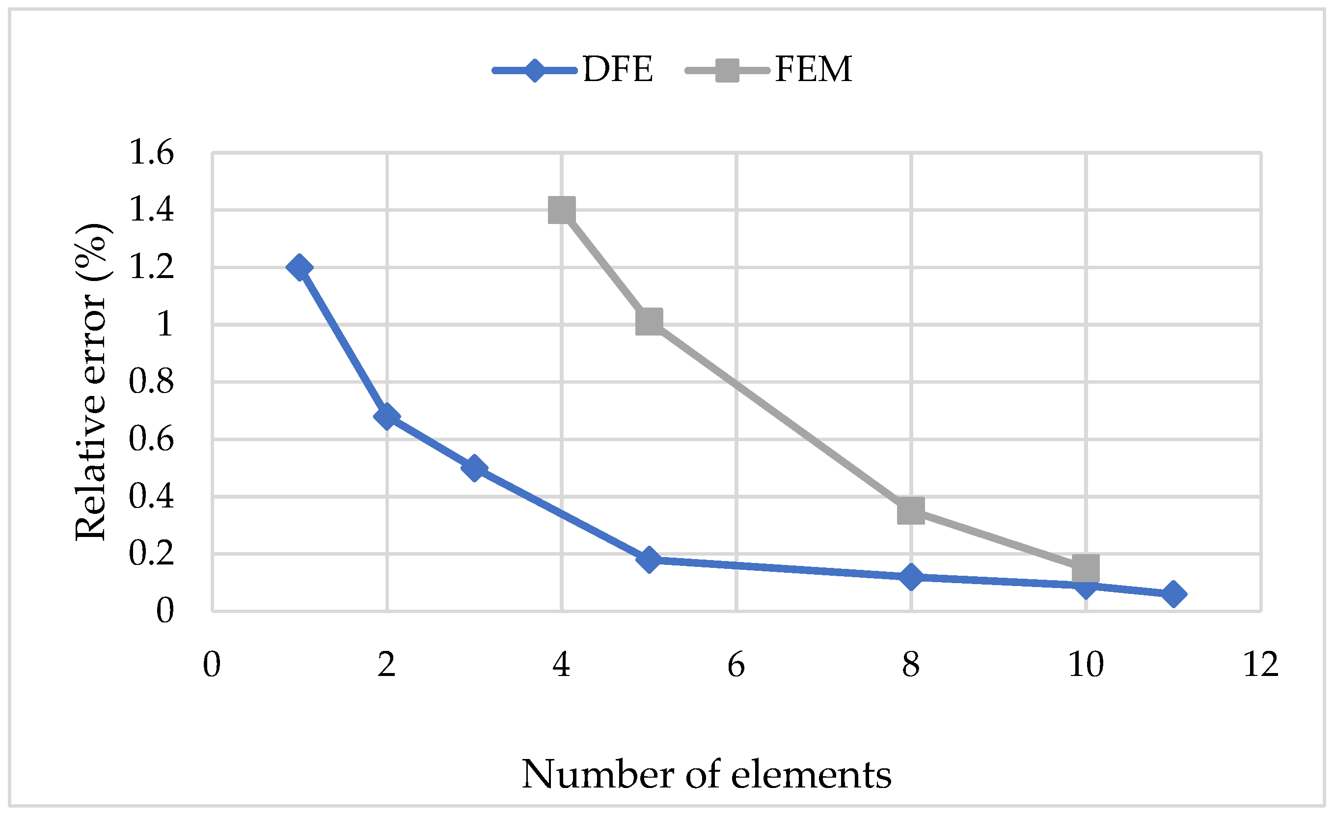
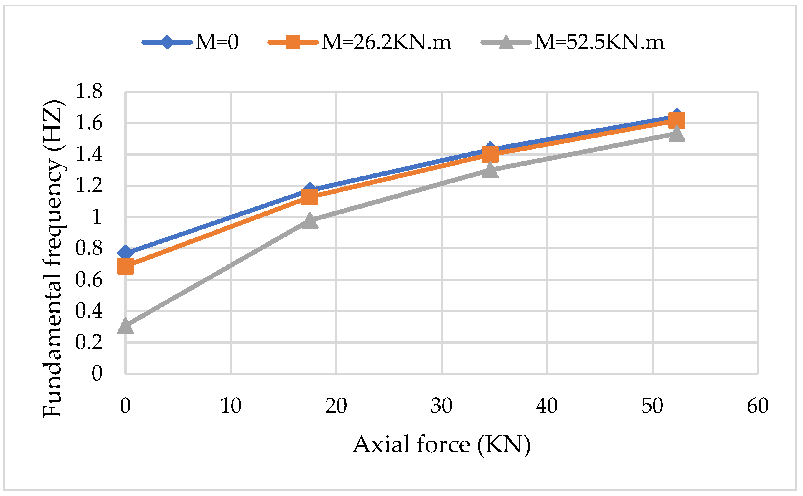
The convergence tests for the two proposed layered beam FEM and DFE formulations are shown in Figure 3, where the DFE rates of convergence surpass FEM by almost a factor of five. An analysis is also carried out to investigate the effects of both axial force and end moment (combined) on the fundamental frequencies of the beam. Figure 4 illustrates the variation of the first natural frequency with tensile axial force and end moment using the DFE method.

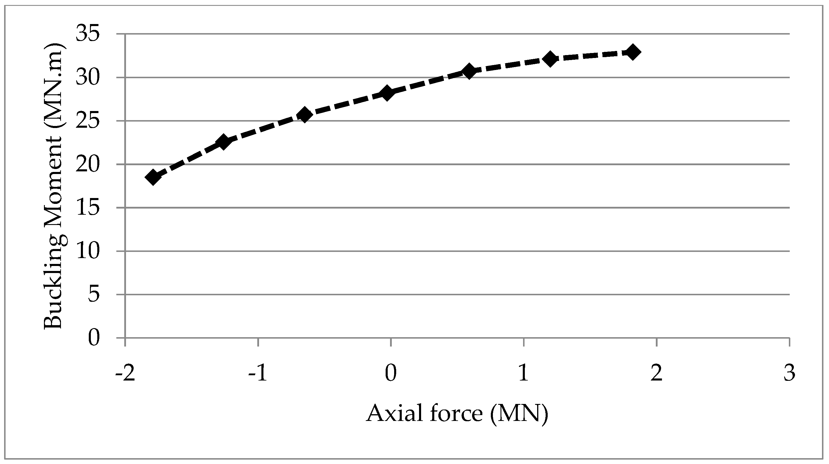
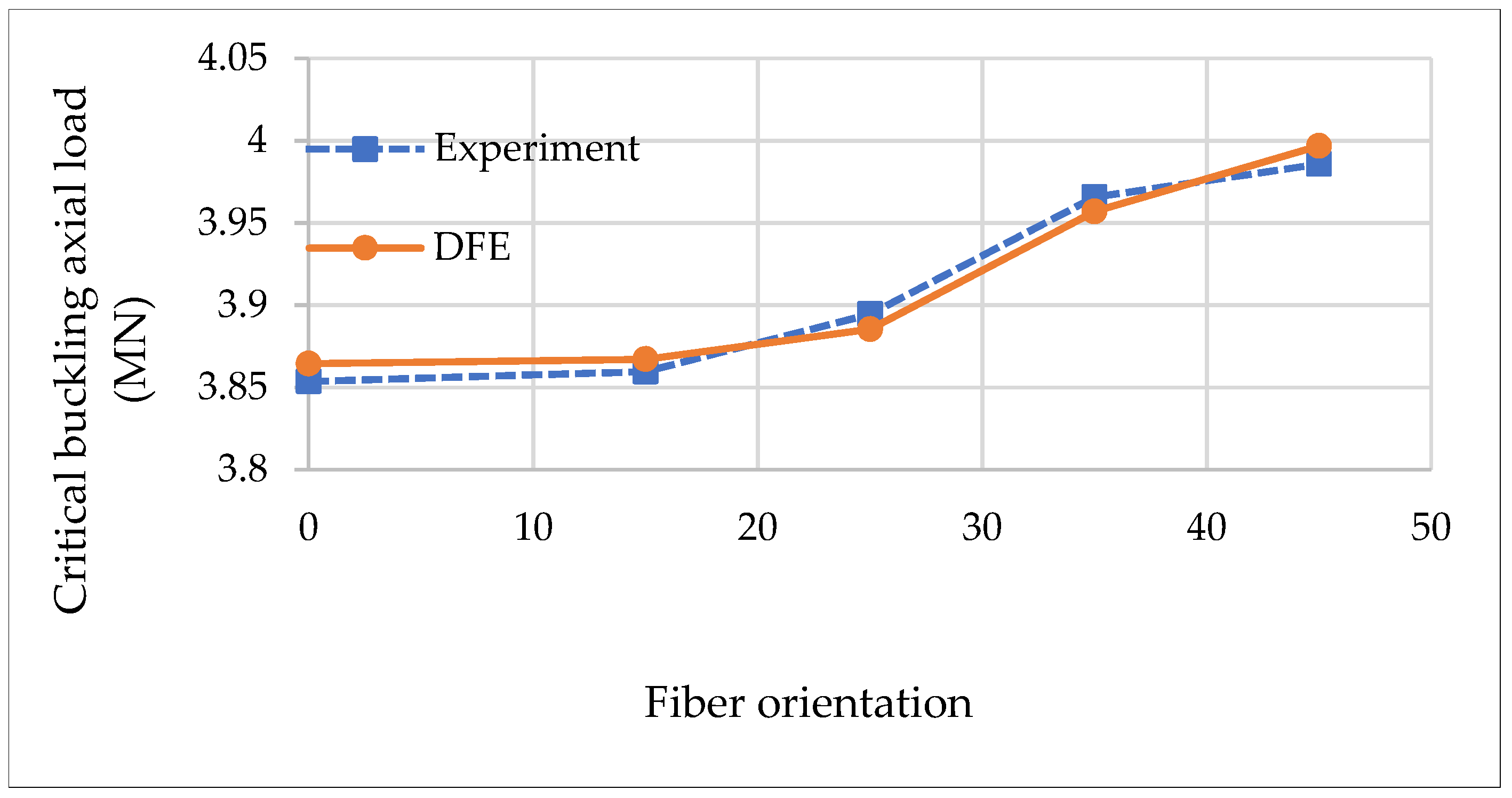
It is possible to use the modal analysis to find critical axial force or critical end moment causing buckling by keeping one of them constant and increasing the other one until the fundamental frequency vanishes, i.e., zero stiffness, or static (structural) instability, which means structural failure. The result of this analysis is presented in Figure 5. As the end moment increases, the structure becomes less rigid which requires a lower axial force to buckle. To validate the results of DFE buckling analysis, in Figure 6 a comparison is presented between experimental study [36] and DFE results for different fiber orientations with M_zz = 0.

3.3. Cantilever Three-Layered Laminated Composite Beam

In what follows, two cantilevered uniform three-layered composite beams made of unidirectional plies of glass/epoxy composite material, with fiber angles 0°/+90°/0° (layup 1) and +90°/0°/+90° (layup 2) are investigated. The beams have a length of L = 0.1905 m, a total thickness of 3.18 mm, a width of 12.7 mm, and the thickness of all three layers are equal. The fiber properties are as follows: E_f = 275.6 GPa, G_f = 114.8 GPa, ν_f = 0.2, ρ_f = 1900 kg/m³ and matrix properties are: E_m = 2.76 GPa, G_m = 1.036 GPa, ν_m = 0.33, ρ_m = 1600 kg/m³ and the volume fraction of both layers is 0.8. The free vibration analysis of the system is performed using both LBFEM and LBDFE methods as well as ANSYS. The first five natural frequencies of laminated composite beams are shown in

Table 4. First five natural frequencies of cantilevered, preloaded, three-layer, unidirectional composite beams (Layups 1 and 2) in Hertz, obtained from 5-element LBDFE and LBFEM, and 20-element ANSYS models, subjected to an axial load of 1.85 MN and end moment of 6.14 MN·m.

Nat. Freq. [Hz]	LBDFE (5 Elements)		LBFEM (5 Elements)		ANSYS (20 Elements)
	layup 1	layup 2	layup 1	layup 2	layup 1	layup 2
1st	79.84	72.35	79.90	72.42	79.84	72.35
2nd	328.05	299.75	342.62	312.04	326.91	298.73
3rd	765.28	736.82	790.48	754.44	757.86	729.74
4th	1274.45	1211.73	1329.06	1266.93	1262.36	1198.44
5th	1387.52	1324.13	1428.38	1377.54	1374.86	1310.99

.

Based on the frequency results presented in Table 3, the LBDFE frequency values for both layups are in excellent agreement with those obtained from ANSYS and LBFEM, with the DFE rates of convergence surpassing FEM. As can be observed from Table 3, for the fundamental frequency the LBDFE and ANSYS results match perfectly, whereas the LBFEM shows a minor difference of less than 0.1%. As expected, as the frequency number increases, the difference between the presented methods and benchmark data increases. Finally, the maximum difference between the LBDFE and ANSYS results (for the 5th frequency) is less than 1%, whereas, for the same number of elements, the LBFEM shows a larger difference of 3.3%.

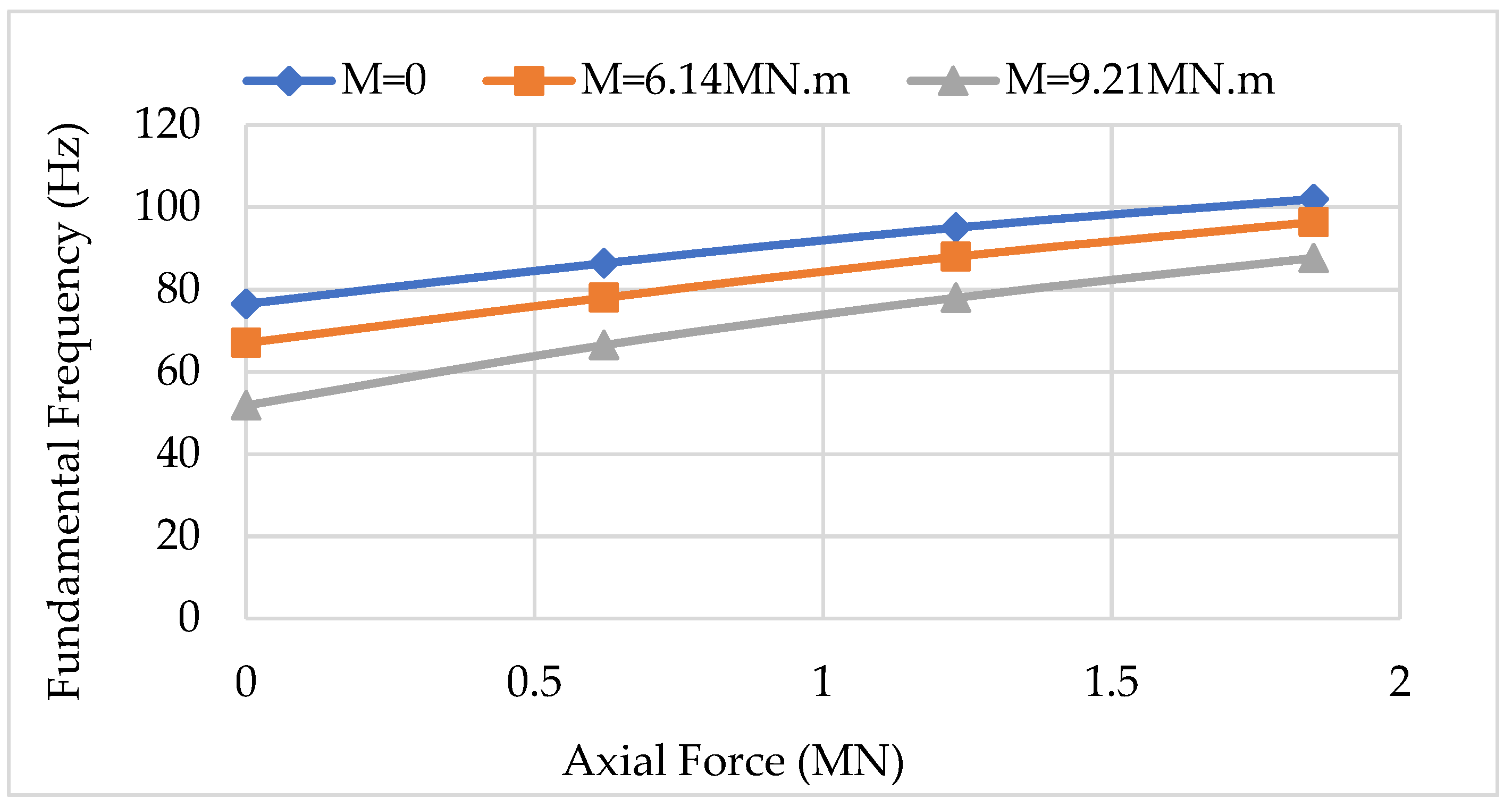
A parametric study is also carried out to examine the variation of the system’s natural frequencies with axial load and end moment. Change of the fundamental frequency of cantilevered, preloaded, three-layer, unidirectional composite beam (Layup 1) obtained from a 5-element LBDFE model, with axial load and end moment is presented in Figure 7. As can be observed, when the axial force is increased, the natural frequency decreases. However, as the end moment is increased, the system’s frequency decreases.

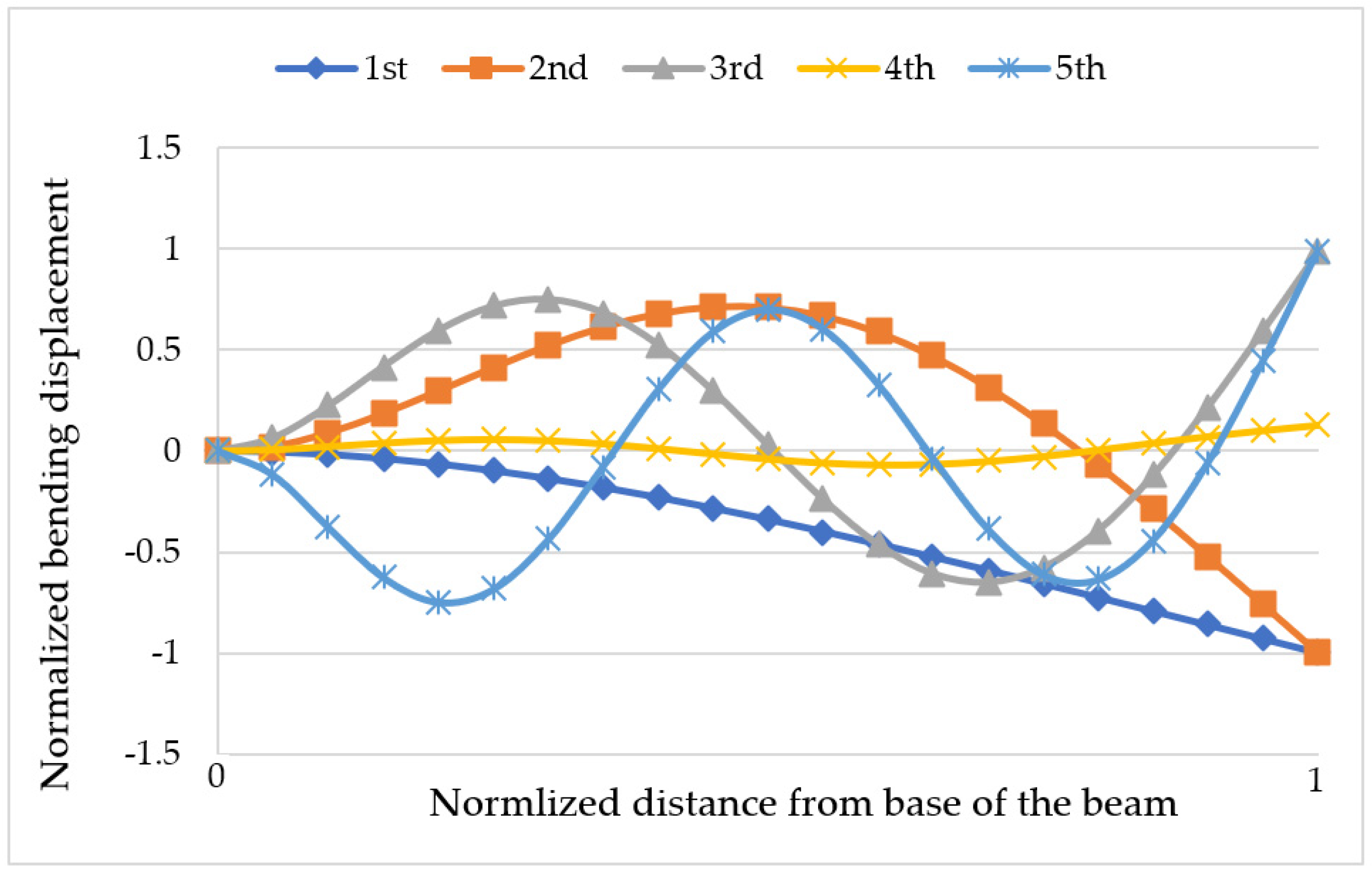
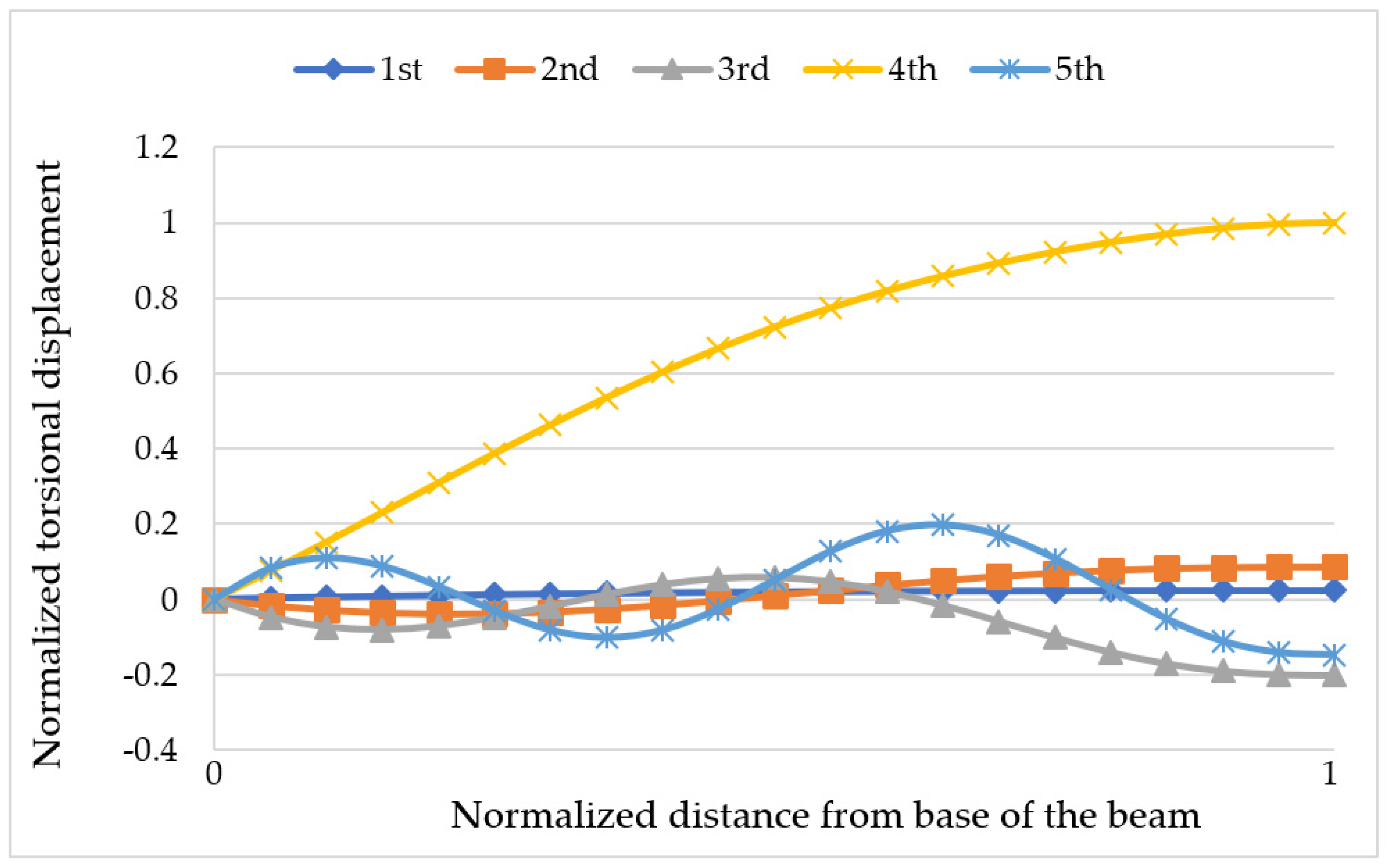
Figure 8 and Figure 9, respectively, show bending and torsional components of the first five mode shapes of the cantilevered, preloaded, three-layer, unidirectional composite beam (Layup 1) obtained using a 20-element LBDFE model, subjected to an axial load of 1.85 MN and end moment of 6.14 MN·m. The horizontal axis represents the normalized distance from the fixed end of the beam (x/L). As can be seen from the figures, the first three and fifth modes are predominantly bending with a slight influence of torsion, whereas the third mode has a predominant torsional character.

4. Discussion

The free vibration analysis of Fiber-Metal Laminated (FML) and unidirectional composite beams subjected to axial force and end moment is presented using layered Finite Element Method (FEM) and Dynamic Finite Element (DFE) models. The frequency results are compared with those obtained from the conventional FEM (ANSYS) as well as the homogenization technique. Based on the results shown in Table 1, the presented layered FEM method has higher a rate of convergence compared to the method of homogenization while DFE has a higher rate of convergence compared to the FEM method, which makes DFE the most efficient method. Considering the benchmark, the estimated error of the FML beam fundamental frequency for the DFE method using five elements along the beam length is almost zero. This error for the layered FEM method using five elements, is around 0.64% while for the method of homogenization using the same number of longitudinal elements it is 2.24%. As expected, and with reference to Figure 3 and Figure 6 (three-layer unidirectional glass/epoxy composite beam, layup 1), the tensile axial load increases the natural frequencies of the beam, indicating an increase in the stiffness of the beam. When the end moment is increased, the natural frequencies reduce, indicating a reduction in the stiffness of the beam. If the end moment is held constant and the tensile load is increased, the natural frequencies increase indicating an increase in the beam stiffness. Conversely, if the tensile load is held constant and the end moment is increased, the beam stiffness reduces. Considering Figure 7 and Figure 8, the coupled vibration of the beam is found to be predominantly flexural in the first few natural frequencies (the first three, for the case studied here) and torsion becomes predominant at a higher natural frequency starting from the fourth mode.

In summary, in all cases studied in this paper, the convergence rates obtained from frequency-dependent Dynamic Finite Element (DFE) formulation are found to surpass those found from the conventional FEM, which in turn surpass the method of homogenization. The higher convergence rate of DFE is mainly attributed to the usage of the solutions to the uncoupled part of equations as the basis functions of approximation space. In comparison with conventional FEM, which uses simple polynomial shape functions, the interpolation functions derived from these solutions provide much better approximations for element displacements expressed in terms of nodal displacements. This higher rate of convergence means that in order to reach a specific accuracy, DFE requires a much smaller number of elements than FEM. This might not look like a huge advantage in the analysis of simple structures like the ones studied here but in large–scale designs of complex systems using DFE would lead to much less computation time.

It is also worth mentioning that the developed conventional and dynamic FEMs here have advantages over FEM based software, ANSYS in modeling prestressed beams, since here the axial force and end moment are included in the equations of motion. Therefore, the developed FEMs give the natural frequency and mode shapes of vibration directly. To use the modal analysis in ANSYS for a prestressed structure, however, one needs to first solve the problem statically. Then, the results of static analysis are to be used to find the new stiffness of the prestressed structure, which will be used later in modal mode to find natural frequencies.

In this study, the effect of interlayer slip was not considered. So, as a proposed future work, the interlayer slip can be added to the DFE model of layered beams subjected to axial force and end moment.

References

- Neogy, J.; Murthy, M.K.S. Determination of fundamental natural frequencies of axially loaded columns and frames. J. Inst. Eng. 1969, 49, 203–212. [Google Scholar]
- Prasad, K.S.R.K.; Krishnamurthy, A.; Mahabaliraja, A.V. Iterative type Rayleigh-Ritz method for natural vibration. Am. Inst. Aeronaut. Astronaut. J. 1970, 8, 1884–1886. [Google Scholar] [CrossRef]
- Timoshenko, S. Vibration Problems in Engineering; Van Nostrand: Opelika, AL, USA, 1964. [Google Scholar]
- Williams, F.W.; Banerjee, J.R. Flexural vibration of axially loaded beams with linear or parabolic taper. J. Sound Vib. 1985, 99, 121–138. [Google Scholar] [CrossRef]
- SHashemi, M.; Richard, J.M. Free Vibration Analysis of Axially Loaded Bending-Torsion Coupled Beams—A Dynamic Finite Element (DFE). Comput. Struct. 2000, 77, 711–724. [Google Scholar] [CrossRef]
- Banerjee, J.R. Explicit modal analysis of axially loaded composite Timoshenko beams using symbolic computation. J. Aircr. 2002, 39, 909–912. [Google Scholar] [CrossRef]
- Hashemi, S.M.; Roach, A. Dynamic Finite Element Analysis of Extensional-Torsional Coupled Vibration in Nonuniform Composite Beams. Appl. Compos. Mater. 2011, 18, 521–538. [Google Scholar] [CrossRef]
- Gellert, M.; Gluck, J. The influence of axial load on eigenfrequencies of a vibrating lateral restraint cantilever. Int. J. Mech. Sci. 1972, 14, 723–728. [Google Scholar] [CrossRef]
- Tarnai, T. Variational methods for analysis of lateral buckling of beams hung at both ends. Int. J. Mech. Sci. 1979, 21, 329–335. [Google Scholar] [CrossRef]
- Banerjee, J.R.; Williams, F.W. Coupled bending—Torsional dynamic stiffness matrix of an axially loaded Timoshenko beam element. Int. J. Solids Struct. 1994, 31, 749–762. [Google Scholar] [CrossRef]
- Leung, A.Y.T. Natural shape functions of a compressed Vlasov element. Thin-Walled Struct. 1991, 11, 431–438. [Google Scholar] [CrossRef]
- Joshi, B.; Suryanarayan, S. Coupled flexural—Torsional vibration of beams in the presence of static axial loads and end moments. J. Sound Vib. 1984, 92, 583–589. [Google Scholar] [CrossRef]
- Joshi, A.; Suryanarayan, S. Unified Analytical Solution for Various Boundary Conditions for the Coupled Flexural-torsional Vibration of Beams Subjected to Axial Loads and End Moments. J. Sound Vib. 1989, 129, 313–326. [Google Scholar] [CrossRef]
- Joshi, A.; Suryanarayan, S. Iterative method for coupled flexural–torsional vibration of initially stressed beams. J. Sound Vib. 1991, 146, 81–92. [Google Scholar] [CrossRef]
- Williams, F.W.; Kennedy, D. Exact dynamic member stiffnesses for a beam on an elastic foundation. Earthq. Eng. Struct. Dyn. 1987, 15, 133–136. [Google Scholar] [CrossRef]
- Issa, M.S. Natural frequencies of continuous curved beams on Winkler-type foundation. J. Sound Vib. 1988, 127, 291–301. [Google Scholar] [CrossRef]
- Mei, C. Coupled vibrations of thin-walled beams of open section using the finite element method. Int. J. Mech. Sci. 1970, 12, 883–891. [Google Scholar] [CrossRef]
- Banerjee, J.R.; Fisher, S.A. Coupled bending-torsional dynamic stiffness matrix for axially loaded beam elements. Int. J. Numer. Methods Eng. 1992, 33, 739–751. [Google Scholar] [CrossRef]
- Hashemi, S.M. Free-Vibrational Analysis of Rotating Beam-Like Structures: A Dynamic Finite Element Approach. Ph.D. Thesis, Department of Mechanical Engineering, Laval University, Quebec, QC, Canada, 1998. [Google Scholar]
- Hasim, K.A. Isogeometric static analysis of laminated composite plane beams by using refined zigzag theory. Compos. Struct. 2018, 186, 365–374. [Google Scholar] [CrossRef]
- Kefal, A.; Hasim, K.A.; Yildiz, M. A novel isogeometric beam element based on mixed form of refined zigzag theory for thick sandwich and multilayered composite beams. Compos. Part B Eng. 2019, 167, 100–121. [Google Scholar] [CrossRef]
- Foraboschi, P. Analytical Solution of Two-Layer Beam Taking into Account Nonlinear Interlayer Slip. J. Eng. Mech. 2009, 135, 124–139. [Google Scholar] [CrossRef]
- Čas, B.; Planinc, I.; Schnabl, S. Analytical solution of three-dimensional two-layer composite beam with interlayer slips. Eng. Struct. 2018, 173, 269–282. [Google Scholar] [CrossRef]
- Cortés, F.; Sarría, I. Dynamic Analysis of Three-Layer Sandwich Beams with Thick Viscoelastic Damping Core for Finite Element Applications. Shock Vib. 2015, 2015, 736256. [Google Scholar] [CrossRef] [Green Version]
- Ross, D.; Kerwin, E.M.; Ungar, E.E. Damping of plate flexural vibration by means of viscoelastic laminae. In Structural Damping, Section II; ASME: New York, NY, USA, 1959. [Google Scholar]
- Mohri, F.; Azrar, L.; Potier-Ferry, M. Vibration analysis of buckled thin-walled beams with open sections. J. Sound Vib. 2004, 275, 434–446. [Google Scholar] [CrossRef]
- Franzoni, F.; de Almeida, S.F.M.; Ferreira, C.A.E. Numerical and Experimental Dynamic Analyses of a Postbuckled Box Beam. AIAA J. 2016, 54, 1987–2003. [Google Scholar] [CrossRef]
- Augello, R.; Daneshkhah, E.; Xu, X.; Carrera, E. Efficient CUF-based method for the vibrations of thin-walled open cross-section beams under compression. J. Sound Vib. 2021, 510, 116232. [Google Scholar] [CrossRef]
- Kashani, M.T.T.; Jayasinghe, S.; Hashemi, S.M. On the flexural-torsional vibration and stability of beams subjected to axial load and end moment. Shock Vib. 2014, 2014, 153532. [Google Scholar] [CrossRef]
- Kashani, M.T.; Jayasinghe, S.; Hashemi, S.M. Dynamic Finite Element Analysis of Bending-Torsion Coupled Beams Subjected to Combined Axial Load and End Moment. Shock Vib. 2015, 2015, 471270. [Google Scholar] [CrossRef] [Green Version]
- Kashani, M.T.; Hashemi, S.M. On the Free Vibration Analysis of Prestressed Fiber-Metal Laminated Beam Elements. In Proceedings of the 15th International Conference on Civil, Structural and Environmental Engineering Computing, Prague, Czech Republic, 1–4 September 2015; Kruis, J., Tsompanakis, Y., Topping, B.H.V., Eds.; Civil-Comp Press: Stirlingshire, UK, 2015; p. 107. [Google Scholar] [CrossRef]
- ANSYS, Inc. ANSYS® Academic Research, Release 13.0, Help System, Coupled Field Analysis Guide; ANSYS Inc.: Canonsburg, PA, USA, 2010. [Google Scholar]
- Bathe, K.-J. Finite Element Procedures in Engineering Analysis; Prentice Hall: Hoboken, NJ, USA, 1982. [Google Scholar]
- Wittrick, W.H.; Williams, F.W. A General Algorithm for Computing Natural Frequencies of Elastic Structures. Q. J. Mech. Appl. Math. 1971, 24, 263–284. [Google Scholar] [CrossRef]
- Banerjee, J.R.; Cheung, C.W.; Morishima, R.; Perera, M.; Njuguna, J. Free vibration of a three-layered sandwich beam using the dynamic stiffness method and experiment. Int. J. Solids Struct. 2007, 44, 7543–7563. [Google Scholar] [CrossRef] [Green Version]
- Plantema, F. Sandwich Construction: The Bending and Buckling of Sandwich Beams, Plates, and Shells; Wiley: New York, NY, USA, 1966. [Google Scholar]
Figure 1.
3-Layered Beam, with axial load and end-moment applied at x = 0 and x = L; Sf represents transverse shearing force. (a) The loads on an element of beam of length δx, and (b) The coordinate system and loadings.
Figure 2.
Discretized domain along the beam span using N elements and 3 DOF per node. The dotted line is used to show that there are more elements than shown in the figure, before and after the element at the middle.
Figure 3.
The convergence study for the two proposed LBFEM and LBDFE formulations; relative error of fundamental frequency for cantilevered FML three-layer beam subjected to an axial load of 17.5 MN and end moment of 52.5 KN·m.
Figure 4.
Fundamental frequency vs. tensile force and end moment for the cantilevered three-layer FML beam.
Figure 5.
Buckling analysis for three-layer FML cantilevered beam using 5-element DFE.
Figure 6.
Critical buckling load vs. fiber orientation for FML using DFE with Mzz = 0, in comparison with experimental results [36].
Figure 7.
Fundamental frequency of cantilevered, preloaded, three-layer, unidirectional composite beam (Layup 1) obtained from a 5-element LBDFE model, subjected to various axial loads and end moments.
Figure 8.
Bending component of the first five mode shapes of the cantilevered, preloaded, three-layer, unidirectional composite beam (Layup 1) obtained using a 20-element LBDFE model, subjected to an axial load of 1.85 MN and end moment of 6.14 MN·m.
Figure 9.
Torsion component of the first five mode shapes of the cantilevered, preloaded, three-layer, unidirectional composite beam (Layup 1) obtained using a 20-element LBDFE model, subjected to an axial load of 1.85 MN and end moment of 6.14 MN·m.