
An Integrated Approach for Failure Analysis of Natural Gas Transmission Pipeline


Industrial Systems Engineering, University of Regina, Regina, SK S4S 0A2, Canada
*
Author to whom correspondence should be addressed.
CivilEng 2021, 2(1), 87-119; https://0-doi-org.brum.beds.ac.uk/10.3390/civileng2010006
Submission received: 4 December 2020
/
Revised: 15 January 2021
/
Accepted: 18 January 2021
/
Published: 1 February 2021
(This article belongs to the Special Issue Addressing Risk in Engineering Asset Management)
Abstract
:The main aim of this study is to identify the most important natural gas pipeline failure causes and interrelation analysis. In this research, the rough analytic hierarchy process (Rough-AHP) is used to identify the natural gas pipeline failure causes rank order. Then a combination of rough decision-making trial and evaluation laboratory (DEMATEL) and interpretive structural modeling (ISM) method is applied to generate the level of importance. The comparison of traditional DEMATEL and Rough-DEMATEL are also performed to establish the cause-effect interrelation diagram. Finally, the Bayesian Belief Network (BBN) is combined with Rough DEMATEL and ISM to identify the interrelation analysis among the most crucial failure causes. As a result, the energy supply company and government policymaker can take necessary safety plan and improve the operation. The main outcome of this study is to improve the security management and reduce the potential failure risks.
1. Introduction
In 2017, Statistics Canada illustrates that the natural gas consumption rates are 14% for commercial, 18% for domestic, and the remaining 68% for industrial sectors. Now, natural gas demand has been growing exponentially in Canada. Natural gas is predicted to increase 43% worldwide by 2040 [1].
The recent statistical analysis indicates that Canada has huge natural gas resources. As per the current consumption rate approximately the next three hundred (300) years Canada has enough reserved [1]. According to the Canadian Energy Regulator (CER) (2020), the length of Canada’s pipelines transporting hydrocarbons like oil and natural gas is 760,000 km (km) and almost 10% (73,000 km) high transmission natural gas pipelines are regulated by CER [2]. The CER regulated the high transmission natural gas pipelines in cross provincial borders, whereas distribution natural gas pipelines are operated by local distribution companies. Millions of Canadian rely on natural gas for cooking, space heating, water heating, etc. As per the Canadian Association of Petroleum Producers (CAPP) analysis, 10 billion cubic feet per day (Bcf/d) of natural gas was consumed in 2018.
Mostly, natural gas is in high demand for residential and industrial users. According to the financial analysis, which was conducted by the Canadian Energy Research Institute (CERI) in 2019, the total Canadian Gross Domestic Product (GDP) of $249.2 billion will be contributed from 2019 to 2029 by the natural gas industry [1].
The complex pipeline structures are used to supply natural gas from the production point to the consumer. It is stated that the high transmission pipeline, whose diameter is large can produce maximum operating pressure (MOP) from 3450 to 6160 KPa. Then the distribution pipeline is operated to deliver natural gas for household and industrial activities [3].
Generally, high transmission long-distance pipeline feeds the distribution pipeline for delivering natural gas in household and industrial activities. In this system, the transmission pipeline is connected with many regulator stations. Any types of breakdown through the system may interrupt the operation. To overcome any types of hazards, regulators can isolate a specific section from the supply line.
Recently, Canadian federal agencies are emphasized to predict future pipeline accidents based on historical data as well as to improve the precise and reliable failure data collection procedure [4]. To determine the risk analysis, both probability of natural gas pipeline failure causes and consequence of natural gas pipeline failure are needed to be considered. In the previous studies, overall natural gas pipeline failure causes analysis are not given emphasis jointly. Most of the previous articles deal with oil and gas pipelines together but not specifically for natural gas pipeline failure causes analysis. Most of the failure causes analysis based on the traditional method such as failure probability, fault tree, and statistical historical data [3,5,6] The multi-criteria decision analysis (MCDA) method is essential for comprehensive safety analysis for natural gas pipeline systems engineering. This new decision-making method is necessary for averting gas pipeline accidents [7]. The further simulation technique is essential to verify the key factors of gas pipeline failure [8].
The principal research objective of this study is to develop failure analysis frameworks to improve the management of the natural gas pipeline. The specific objectives of this research are:
- To develop natural gas transmission pipeline failure risk analysis models with limited failure data.
- To establish a methodology for identifying the contextual relationship among the natural gas transmission failure causes with the help of academic and industrial experts’ opinions.
- To integrate rough set theory with existing MCDA methods and Bayesian belief network (BBN) for considering model uncertainties due to limited failure information and the vagueness in the experts’ judgments.
After the introduction section, this research work consists of several sections as follows. In literature review, the current literature is reviewed, which deals with natural gas pipeline failure causes analysis. Next, the overall methodology for this paper is described in Section 3. Thereafter, the overall frameworks are labeled in Section 4. Then the framework implementation in Section 5 and results and discussion are demonstrated, and the overall analysis are explained in Section 6. Lastly, the conclusion, recommendation, and limitations, and future research scope are given in Section 7.
2. Literature Review
This chapter represents the natural gas failure causes related to the research and limitations. The literature review consists mainly of two parts as such failure causes and present methodology. In this literature review (first part), failure causes are analyzed by two subsequent parts such as failure causes and the methodology.
2.1. Natural Gas Pipeline Failure
Generally, natural gas contains methane along with a small portion of propane, ethane, and sulfur gases. If natural gas concentration reaches 5%, in that case, a fire explosion will occur [9]. Natural gas pipeline failure events data can determine the weak point of the gas pipeline. The natural gas pipeline leak may result in air quality decoration, fire explosion, human casualties, and economic penalties. To identify the causes, sensitive point analysis of gas pipeline failure can reduce the potential risk and enhance safety integrity for preventing the accident.
As per EGIG (European Gas Pipeline Incident Data Group) analysis, the three major gas pipeline failures causes are pipe/weld material failure, excavation damage, and corrosion. If the gas pipeline diameter is large with high pressure, in that case, the explosion is more catastrophic compared to a small diameter pipeline [10].
In natural gas pipeline failure events, one of the causes is weld/pipe material failure under the category of manufacturing and construction defects. Because of the advanced technology and improvement of management quality, the pipeline structural defects can be eliminated. Though sometimes it is not possible to give assurance to the construction quality because of several external and internal constraints [10].
Despite all the technological advancement, still, in many cases, a certain number of defects are present, such as weld, gouges, and dents. The economically active areas around the globe are mostly affected by third-party damage (TPD). In 2016, a report indicates that five Canadian provinces, such as Saskatchewan, Ontario, British Columbia, Alberta, and Quebec indicated 91,539 incident reports on the distribution of natural gas pipelines for TPD [11].
In one of the provinces in Canada, Ontario, approximately 80% of distribution gas pipeline operates under MOP at 420 kPa. Those pipes’ material compositions are polyethylene plastic (PE). Mostly, NPS2 small diameter category pipes are used for gas distribution. As per PHMSA gas pipeline failure analysis since 1984 states that the TPD is responsible for above 50% of gas pipeline incidents [11].
As per PNGPC (PetroChina Natural Gas & Pipeline Company, China), statistical analysis is almost the same as other overseas organizations. Still, lots of improvements are required for instance construction and manufacturing quality and monitoring technique of third-party activities [10].
During gas transmission through the long-distance gas pipeline, energy and pressure are comparatively high. In most cases rupture and crack happen because of the operation faults, corrosion, and material defects [9].
Natural gas transmission aging pipeline wall thinning (deterioration) is caused by corrosion. It is one of the severe operational hazards and pipeline degradation rates may vary expressively. In accordance with classes, inline inspection (non-destructive test) results are required for probabilistic pipeline failure estimations analysis [11].
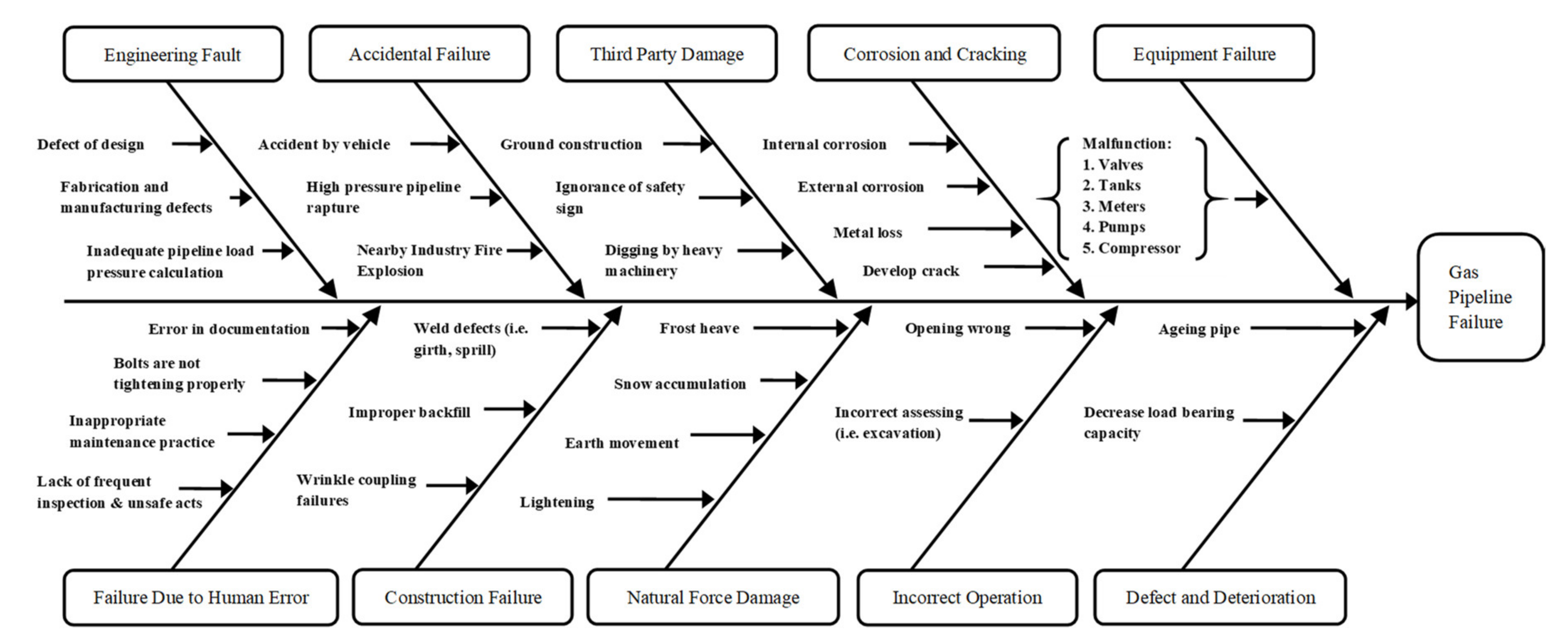
The “natural gas pipeline failure” causes summary (Figure 1) fishbone diagram is generated based on literature review and open data sources and experts’ opinion. This figure represents the overall failure causes as described earlier of natural gas pipeline failure along with the root causes. Generally, this diagram gives an overview further of natural gas pipeline failure causes analysis. Table 1 also summarizes the gas pipeline failure causes.
2.2. Present Methodology
One of the main limitations of gas pipeline failure risk analysis is the lack of data. For this reason, the experts’ opinion is required to assess the failure causes probability. To analyze the failure events, linguistic terms are used such as “very low”, “low”, “medium”, “high”, “and very high” [9].
A systematic scientific approach can eliminate and prevent the accident rate. In recent years, several quantitative and qualitative methods are implemented for risk assessment of natural gas pipeline failure, such as analytic hierarchy method, probability and statistics method, Bayesian Belief Network (BBN), fault tree analysis (FTA), etc. [9].
The most common method analytic hierarchy process (AHP) is used for rank-order analysis. In cases of ambiguity for the decision-making process, the rough set theory is incorporated with AHP [20]. In pairwise comparison, rough set theory can be implemented based on lower and upper approximations [21].
Recently, BBN is used to develop the probabilistic risk model to exceed the traditional (FTA) method [22]. BBN is proposed for conditional reliance analysis for natural gas pipeline failure accidents [5].
The safety analysis in different respective fields, as well as urban gas pipeline failure factors, are well-established with the help of BBN [23,24]. These networks BBN can be developed from domain experts’ opinions or real incident data analyses [25].
Presently, plotting FTA to BBN is the common approach for risk model analysis, but this integration does not systematically show results on how various causing factors interact with each other [26].
Therefore, this mentioned study has been applied to a hierarchical network model for constructing the decision-making trial and evaluation laboratory (DEMATEL) and interpretive structural modeling (ISM) method to describe the BBN model for gas pipeline accident probability study [8].
The DEMATEL method can identify critical factors and able to develop their causal relationships. This DEMATEL method was established by the “Science and Human Affairs Program of the Battelle Memorial Institute of Geneva”. The causal relationship among the elements in a particular system of the DEMATEL model is represented by a digraph. This digraph mainly determines the strengths and influence of the factors. To understand the cause–effect relationships between causal dimensions, factors are analyzed by using digraphs in DEMATEL methodology [27].
The main influential indicators were evaluated and identified based on the expert’s valuable opinion. Thereafter a pairwise comparison matrix was used in the DEMATEL method. Basically, DEMATEL was used in several selection processes in complex problems [28]. The DEMATEL method can analyze the interrelationship as well as define the strength of contextual relations in the system [29]. The cause and effect model was used to recognize the indirect relations in the DEMATEL method [27]. In addition, the DEMATEL method can determine the relationships between direct and indirect dependencies in complex problems [30].
The DEMATEL method can investigate complex group decision-making problems. To improve performance, the DEMATEL methodology can find the main criteria based on decision-making data [31].
In another field of study, DEMATEL and rough set theory methods are combined to analyze the interactions for evaluation of (product-service system) PSS requirement. This combination method can deal with the vagueness of subjective decision for PSS requirements. As a result, this new approach maybe improve the group DEMATEL interaction relationships with a combination of rough set theory for PSS subjective decision. Consequently, the new rough group DEMATEL is more accurate to develop the interaction without enough information compared to the traditional DEMATEL [32].
The rough group DEMATEL method can be implemented in another field of study for critical influences analysis [32]. Also, group decision-makers can decide a vague environment for complex factors analysis. One of the main limitations of the rough group DEMATEL method is that this method does not distinguish between positive and negative influential requirements of PSS [32].
Basically, rough sets are measured based on vagueness data [33]. If the statistical method is not applicable to analyze the system in that case rough set is applicable [34].
In the year 1973, for the first time Warfield proposed the (ISM)-based model. The main objective of this model is to construct a multiple level structural models with the support of industrial experts’ work experience opinion and technical knowledge to analyze several elements in complex system performance [35].
Based on the driving and dependence power, the performance is measured by clustering using the ISM method. Furthermore, MICMAC analysis has been developed using the driving and dependence power. The performance was divided into four clusters such as autonomous, linkage, dependent, and independent [36].
The ISM method is considered as a management decision-support tool for performance measurement analysis. Hence, this ISM model can be used for any decision-making process and analysis. Besides, ISM is able to identify the specific relationship (i.e., problem and issue) among the variables [37,38].
An ISM methodology is used in the automobile service center to identify the different variables and further develop the interrelationship in-between the variables [39]. Also, the ISM model is set up to analyze the causal relationship among the evaluation of vendor performance [27]. A combined qualitative and quantitative data are implemented in the ISM model for the development of a balanced scorecard [40].
The ISM methodology is used in the automobile industry for complex relationship measures of supply chain management with the help of a decision-maker’s value. ISM technique tool can predict an effective action plan for management in complex situations [41].
Another study states that the urban buried gas pipeline network accident-triggering factors orderly approaches with the grouping of three altered methods. Those methods included DEMATEL, ISM, and BBN.
In this study, the DEMATEL method is applied to compute the numerous influences for gas pipeline failure and classify the most critical influential factors. Additionally, the ISM method is integrated with DEMATEL to identify the hierarchical structure of the complex gas pipeline accident-causing factors [8].
Furthermore, the BBN network is implemented to determine the key routes of the conditional probability of occurrence in pipeline system failure. BNB is a theoretical intellectual model, which deals with uncertain knowledge [8].
After reviewing, the different types of existing methodology for natural gas pipeline failure analysis (Table 2) and other recent MCDA methods from different journals are considered in this research to develop the new idea for natural gas pipeline failure causes and interrelation analysis.
3. Methodology
In this study, the ISM method is utilized to structure the natural gas transmission pipeline failure causes at different levels while MICMAC analysis helps classify the failures based on the driving and the dependence power. Rough-analytic hierarchy process (Rough-AHP) method is used to rank the failure causes and Rough-DEMATEL is used to determine the causal relationship between the failure causes under an ambiguous situation. Finally, Rough DEMATEL- ISM methods are integrated with BBN to analyze the various interactions for gas pipeline failure causes. The following sections briefly discuss the methods utilized in this paper.
3.1. ISM Method
ISM technique deals with expert’s opinions to develop a complex system based on a qualitative approach. The entire complex system is developed by a relationship digraph [44]. The following steps are described as calculation procedure:
- Step 1. Establish overall influence matrix H
The overall influence matrix (H) represented as is calculated by adding the unit matrix (I) with the total relation matrix (T). The overall influence matrix is generated as follows:
- Step 2. Develop reachability matrix K and determine the cause-effect relations among the factors
In this stage, each component of matrix (H) signifies exactly how the factor affects factor (here, ). The threshold value can be determined from the reachability matrix. The reachability, matrix ; here means factor straightly affects the factor () can be calculated by using the following equations:
- Step 3. Determine the level of each factor and develop the initial diagram
By using the reachability set and antecedent set , all the factors are divided into different levels. The following equations determined the reachability set and antecedent set:
The antecedent set is the group of all factors that affect the other factors and the factor itself. Oppositely, an intersection set is collected for all the factors that are common in both sets.
- Step 4. Develop the hierarchical network model
A diagraph is generated to demonstrate the relationships among the causes in the expression of edges and nodes. On completion of incongruities check, indirect links are removed and the network nodes are replaced with cause’s descriptions.
MICMAC Analysis
The main objective of the MICMAC analysis is to classify the failure causes based on driving and dependence power though a graphical representation [41]. The graph is divided into four quadrants such as autonomous variables, dependent variables, linkage variables, and independent variables.
- Autonomous variables: This quadrant represents the autonomous variables. In this quadrant, both variables (driving and dependence) have low power.
- Dependent variables: This quadrant contains dependent variables, whereas it holds lower driving and higher dependence power.
- Linkage variables: The linkage variables are expressed in this quadrant. This quadrant has strong driving and strong dependence power. Their action affects others and also possesses a back effect on themselves. The factors affect other factors as well as themselves.
- Independent variables: This quadrant included independent variables considered by higher driving and weak dependency power.
3.2. DEMATEL Method
The DEMATEL method is required to identify the influences among the criteria. In addition, the DEMATEL method is also required to develop a casual relationship diagraph [45]. The following steps are required to calculate the DEMATEL method.
- Step 1. Initial average matrix
In this stage, the pairwise comparison is developed based on linguistic scale value from 1 (No influence) to 4 (Very high influence). In this study, four industrial and academic experts are invited to develop the pair-wise comparison. Here, the notation of indicates the expert’s opinion where affects with the help of integer scores. Now, the average matrix A is represented as follows:
- Step 2. Direct relation (D) matrix
After normalized initial direct relation matrix is acquired by normalizing average matrix (A).
- Step 3. Calculate the total relation matrix (T)
The total relation matrix formula is as following:
Here I = identity matrix, and vectors are demonstrating the sum of rows and columns accordingly of the total relation matrix (T).
- Step 4. Identify the threshold value
In this step, a threshold value is required to get the diagraph. This value indicates how one factor affects another factor. Basically, the threshold value is set up by calculating the average from the elements of (T) matrix. Finally, the casual relationship diagram can be generated with the help of mapping from the dataset of and .
3.3. Rough Set Theory
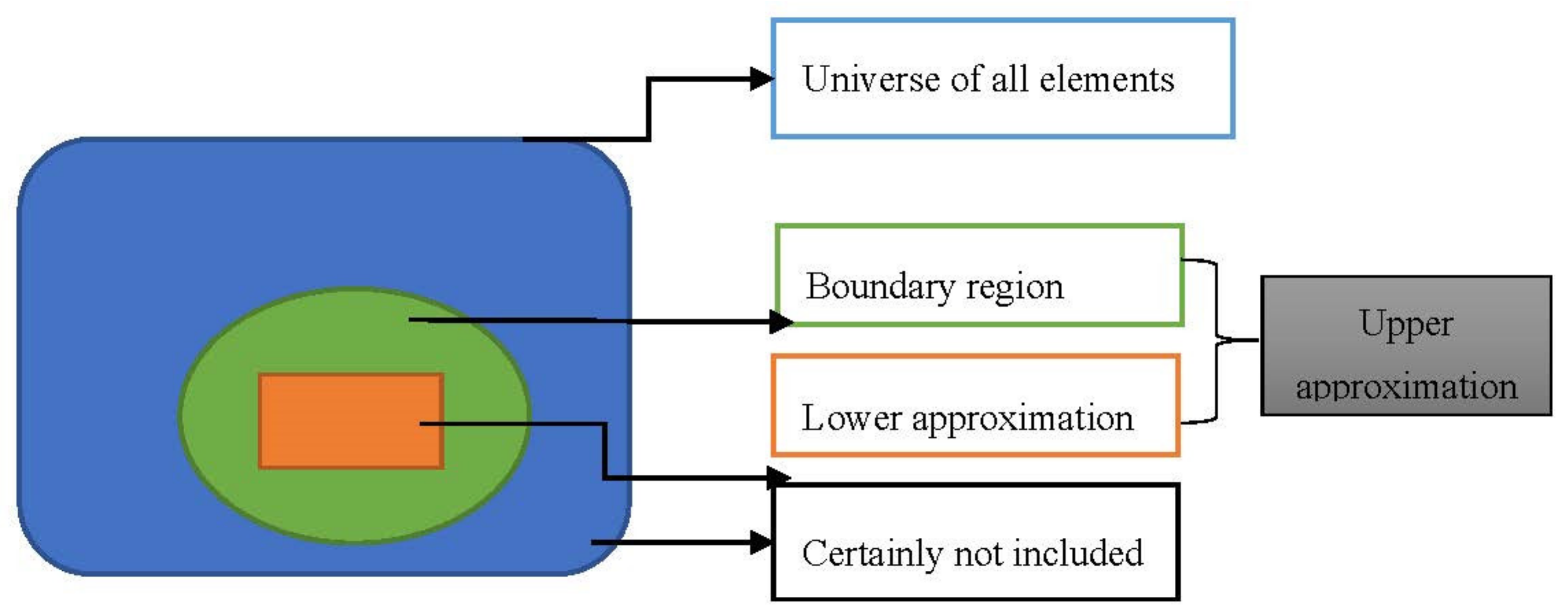
The rough set theory is used to represent any vague idea as a pair of precise perception on the basis of upper and lower approximations (Figure 2). One of the main advantages of rough set theory is that it is able to find the important hidden patterns data [46]. Let, can be represented by a rough number. This rough number can be determined by its corresponding lower limit and upper limit . Let us consider, as the universe, which contains all the objects, is an arbitrary object of . Here, classes set is and cover all the arbitrary objects in . At this point, class order is considered as, .
Thereafter, the lower approximation , upper approximation , and boundary region of class [46] are defined as follows:
The object can be obtained with rough number , which is calculated by its corresponding lower limit and upper limit , respectively:
where, and represent the sum of the objects contained in the lower and upper object approximation of , respectively.
Rough boundary interval :
Application of two rough numbers and as per [47] are:
The rough numbers arithmetic is calculated by the help of the following formula:
Addition of two rough numbers and
Subtraction of the two rough numbers and
Multiplication of the two rough numbers and
Division of the two rough numbers and
Scalar multiplication of rough number , where is a nonzero constant
3.3.1. Rough AHP Method
The AHP is integrated with a rough number to compute the weight of each failure criteria. The Rough-AHP calculation procedures are described as the following [48]:
- Step 1. Classify the criteria, thereafter develop a hierarchical structure with the evaluation objective.
- Step 2. First, conduct a survey from experts’ opinions and develop a group of pair-wise comparison matrix. Here, the pairwise comparison matrix of the expert (eth) is described as follows:
- Step 3. In this step, calculate the maximum Eigenvalue of the (decision matrix). Thereafter, calculate consistency index CI by using the following equation.
Then, calculate the consistency ratio from the decision matrix Now, considering the value of random integer from (Table 3) and consistency ratio test by using the following formula:
Inconsistency test, if value is consistent then it should come less than . Otherwise, the pairwise comparison matrix is inconsistent. Then further revision is required from decision-makers. The integrated comparison matrix is constructed as follows:
where, , is the order of relative significance of criterion on criterion .
- Step 4: Develop the rough comparison matrix.
The element will translate into the Then, rough number by using the following equations:
Accordingly, is the lower limit and is the upper limit of .
Then, the rough set numbers sequence is implemented based on the expert’s opinion as follows:
Furthermore, it is translated into an average with the help of rough arithmetic equations,
where consists of is the lower limit and is the upper limit.
Afterward, the rough comparison matrix N is generated as:
- Step 5. Compute the rough weight (Wg) of each criterion:where is the normalized weight of the criterion from the rough set. Then, the criteria weights are obtained.
3.3.2. Rough DEMATEL Method
The DEMATEL method is integrated with rough set theory under vagueness decision-making process without enough information [32]. The calculation steps are described as follows:
- Step-1 Direct relation matrix
In this methodology, the pairwise comparison matrices of four industrial and academic experts are used. Here, and are the lower and upper limits of rough number . Then the final rough group direct-relation matrix is formulated by using Equations (8)–(14) as follows:
- Step-2 Development of Rough total-relation matrix
The linear transformation scale method is applied as a normalization formula. Whereas it compared the decision-making scale to a comparable scale.
- Step-3 Development of the Rough total-relation matrix
= Normalized rough group direct-relation matrix, I is the identity matrix. Then, the rough total-relation matrix T can be obtained as follows:
- Step-4 Development of the ‘‘Prominence” and ‘‘Relation”
In this third step, the sum of rows and columns are individually expressed by and from the rough total relation matrix T as follows:
whereas, is considered as the lower limit and is considered as the upper limit of the rough interval . Then rough interval is considered as the lower and upper limit such as and , accordingly. To efficiently find the prominence and relation, it is necessary to convert and into crisp values. Finally, the de-roughness of is calculated as follows:
Here, and are the normalized equation from and , accordingly.
Total normalized crisp value,
- Step-5: Calculation of final crisp values
In the same way, we can find the final crisp values for for .
Then, add and to find out the prominence vector , next determine the relation vector by subtracting to
If the value is positive then it goes to the cause group and if the value is negative then it goes to the effect group or vice versa. Then the next step, the casual diagram can be developed with the help of a dataset from and . As a result, it provides the decision of the system.
3.4. Integrated Rough DEMATEL-ISM Method
Rough DEMATEL is further proceeded with ISM to identify the level of importance among the relationships. Equations (31)–(44) are applied to compute the Rough DEMATEL. Thereafter, the total relation matrix from Rough DEMATEL is implemented in Equation (1) to identify the overall influence matrix (H) from the ISM method.
3.5. Bayesian Belief Network
The BBN is an effective theoretic model, which is used for complex structure analysis in an uncertain environment [8]. The gas pipeline failure causes hierarchical network model analysis is developed with an integrated Rough DEMATEL-ISM method. Then this hierarchical network is combined with BBN, using Netica software with the help of expert’s advice. Further, the conditional probability table (CPT) is developed with the help of the domain expert’s opinion. The various causing factors interrelation are developed by BBN nodes with the help of CPT values. Based on conditional dependencies and chain rule the joint probability distribution is whereas is calculated as follows:
Here, is the parent set and is the variable. On the basis of Bayes’ theorem, the following relationship evidence is developed,
4. Failure Analysis Framework
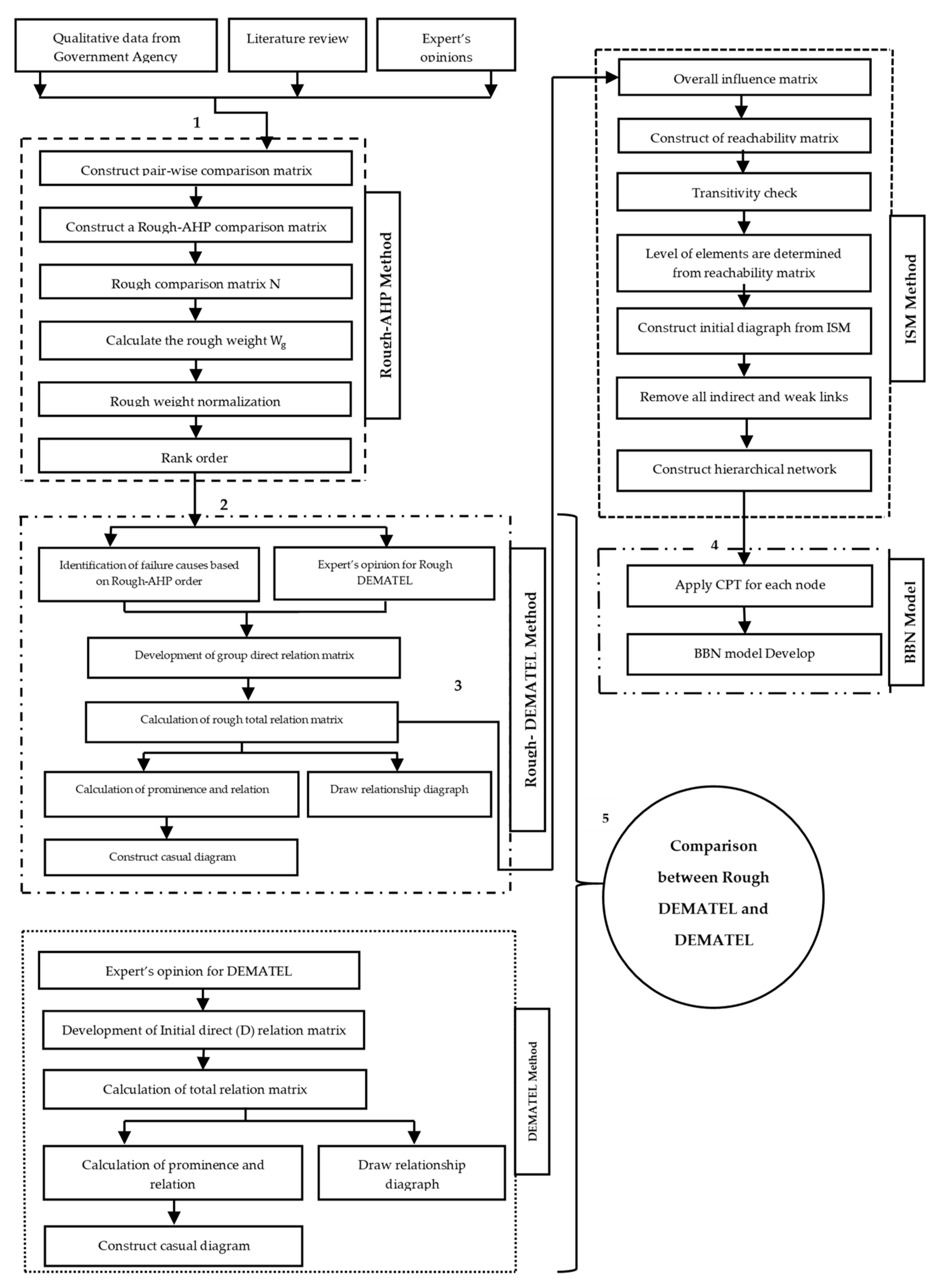
The academic and industrial experts (decision-makers) are interviewed with the help of the questioner and matrix to identify the failure causes and interrelations analysis. In this study, Rough AHP, Rough DEMATEL, DEMATEL, and ISM along with BBN are used to develop the general framework for natural gas pipeline failure cause and interrelation analysis (Figure 3).
5. Framework Implementation
In this section, the proposed natural gas pipeline failure analysis and consequence analysis frameworks are implemented. All the equations mentioned in Section 3 are implemented in this section, to calculate and develop the different types of hierarchical models and graph for failure causes influence analysis.
5.1. Rough-AHP Calculation
The pairwise comparison matrix is formulated by using Equation (20). The decision-maker’s opinions are considered here, such as Extreme Importance-5, Vital Importance-4, Essential Importance-3, Moderate Importance-2, and Equal Importance-1 are considered along with the reciprocal value of this mentioned scale (Appendix A). In Rough-AHP, the pairwise comparison matrix consistency check is required until the value is a pass (<0.10) by using Equation (21) [50]. Thereafter a component for example, (corrosion and cracking) are constructed with the help of four decision-maker’s judgments matrix as follows (1.00, 0.50, 0.50, and 1.00). By using the Equations (8) and (9) the following rough number lower and upper approximation are calculated for :
By using the Equations (11)–(13) the rough number is as following:
After implementing the Equations (8)–(13), the final rough number with the upper and lower limit is as such [0.63, 0.88]. Then the Rough comparison matrix N was constructed by using Equations (20)–(28). The Rough comparison matrix N matrix results are given in Appendix B. In the last step are computed the Rough-AHP Normalized weight (Table 4) with the help of Equations (29) and (30).
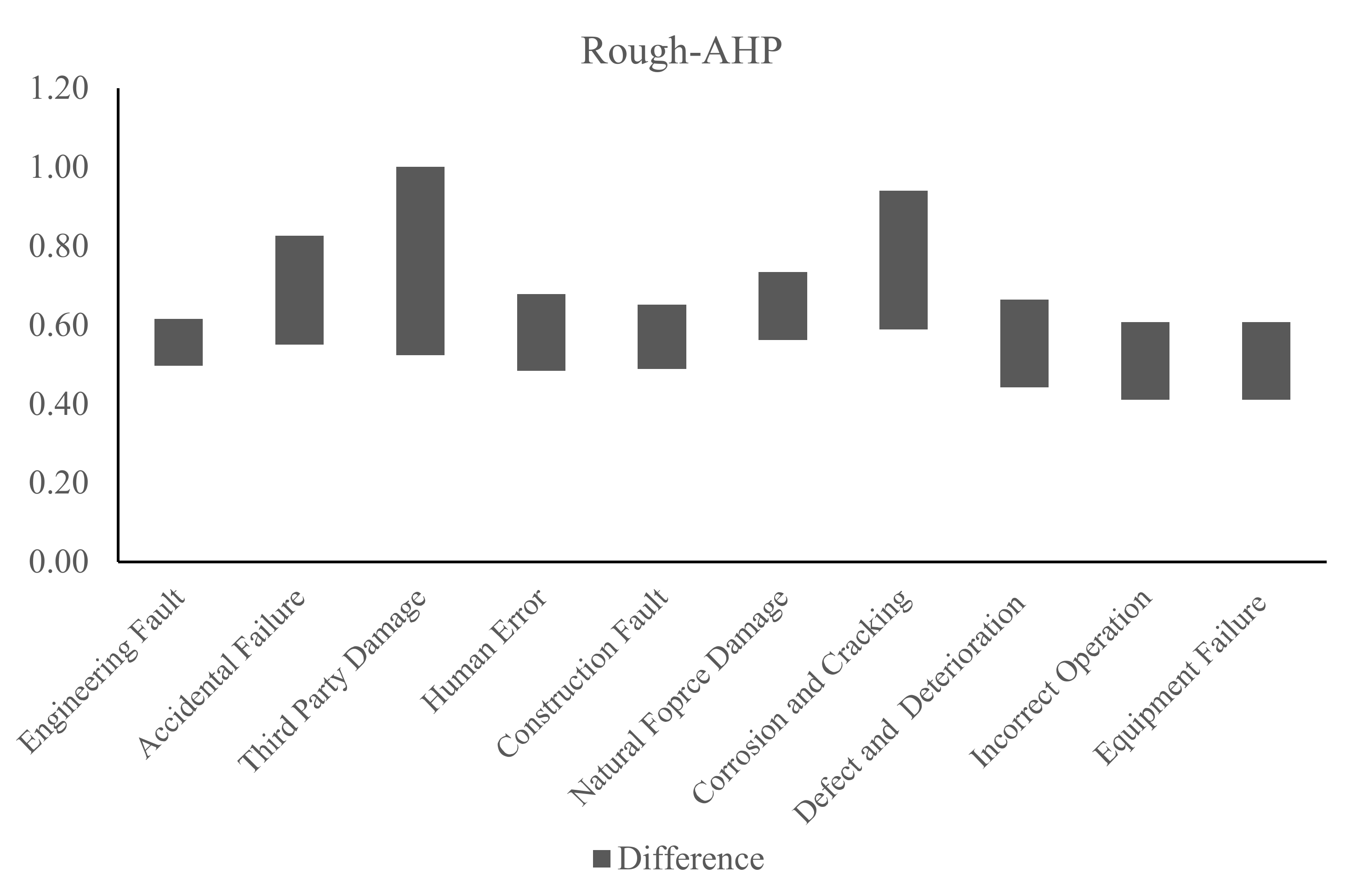
Further, the failure causes rank order is constructed based on the upper and lower limit differences (Table 4 and Figure 4). As per rank order and experts’ opinion, 6 consecutive failures causes are considered for the next level of analysis. Those are according to the rank order as such, Third-party Damage (R1), Corrosion and Cracking (R2), Accidental Failure (R3), Defect and Deterioration (R4), Incorrect Operation (R5), and Equipment Failure (R6).
5.2. Rough-DEMATEL Calculation
In Rough-DEMATEL four experts’ opinions are considered and constructed pairwise comparison based on a scale, such as Very high influence 4, High influence 3, Low influence 2, Very low influence 1, and No Influence 0. The individual decision-maker opinion pairwise comparison matrix is given in Appendix D.
For an instance, for a component (Corrosion and Cracking) the decision-maker judgments are as follows (3, 2, 3, 3). Now, implementing the Equations (8)–(14), the final rough number has the upper and lower limit as such (2.94, 2.56). Then the final rough group direct-relation matrix G is formulated by using Equation (31).
In the next step, the rough-direct relation matrix (Table 5) is the normalized using Equations (31) and (32) and the normalized matrix is shown in Table 6. Then the rough total relation matrix value (Table 7) is obtained by using Equation (31). By using Equations (36) and (37) the development of the “Prominence” and ‘‘Relation” values are computed in (Table 8). Here, indicates the prominence and indicates the relation.
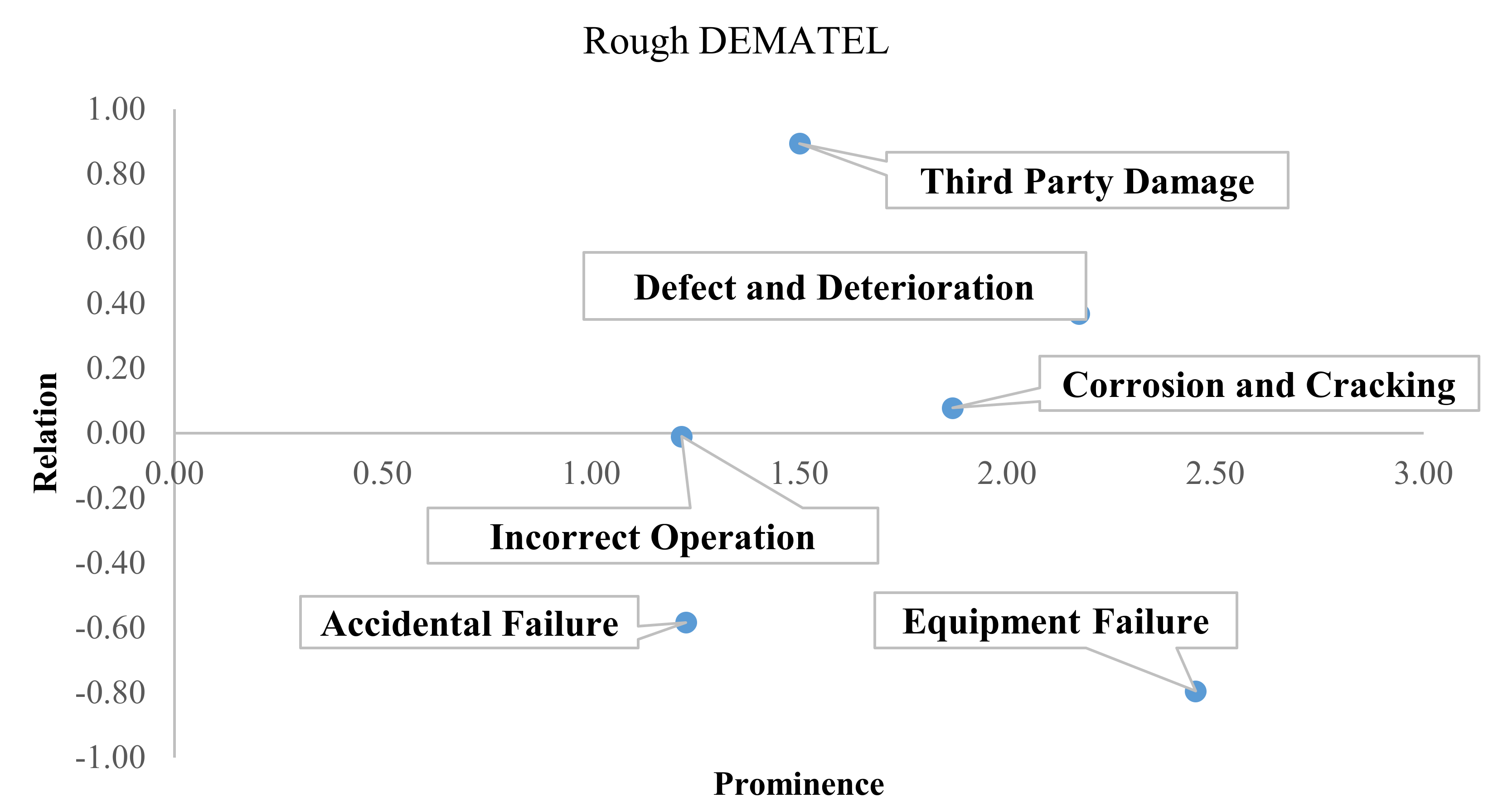
In Figure 5, above the horizontal axis points are considered as a cause group and below the horizontal axis points are measured as an effect group. Finally, the casual relationship graphical representation is drawn as follows:
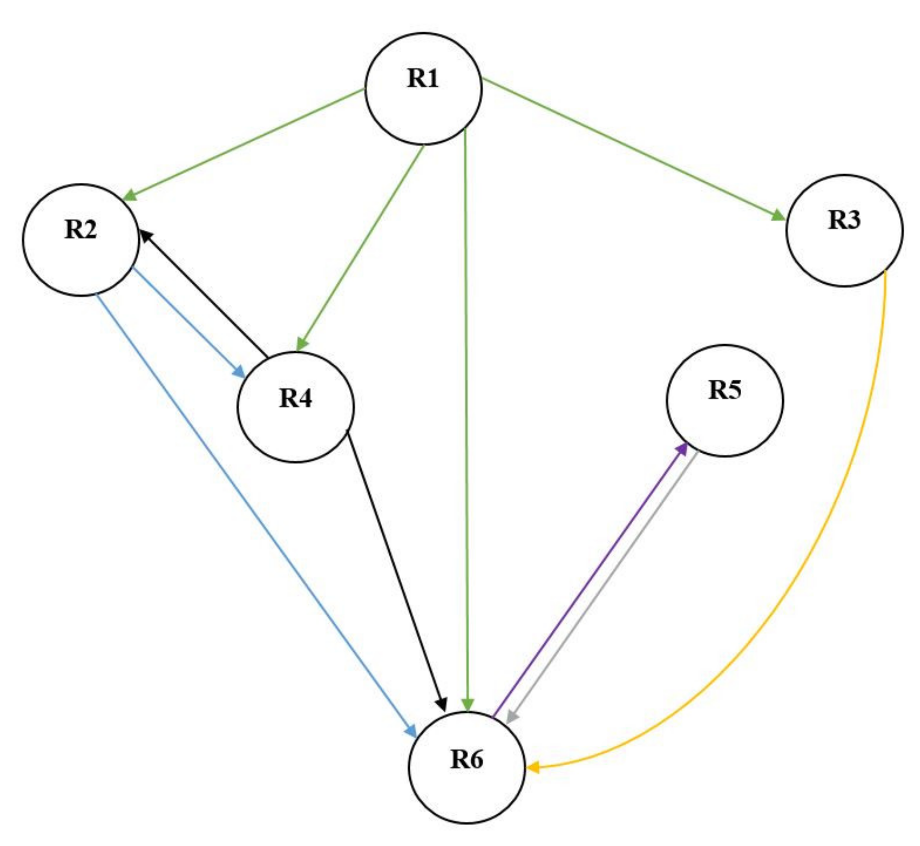
The threshold value is required to develop a Rough DEMATEL relationship diagram in (Figure 6). This value is determined by calculating the average from the average matrix (Table 9). The initial value is found (0.11) from the average matrix. After completion of a number of tests and experts’ opinions, finally, value is selected 0.14 with the help of half stand deviation calculation to reduce the weak links.
In the below (Table 9) average matrix few numerical values are bolded. For example, value compared to (R1) in column and (R2) in row, the value is 0.18 which is bigger than value 0.14. Thereafter, an arrow line goes from (R1) to (R2) likewise the following relationship diagram is being produced (Figure 6) to understand the influence between the causes.
5.3. DEMATEL Calculation
DEMATEL calculation also required the expert’s opinion to construct the initial pairwise average matrix (Appendix D) by using Equation (6). The decision-makers’ opinions are followed by the same scale value as Rough -DEMATEL such as Very high influence 4, High influence 3, Low influence 2, Very low influence 1, and No Influence 0. After normalizing the average matrix value (Table 10). After normalizing the average matrix, the normalized direct relation matrix is obtained from (Table 11). The total direct relation matrix (Table 12) is computed with the help of Equation (7). Step 4 (Section 3) from the DEMATEL method, the “Prominence” and “Relation” values are computed (Table 13).
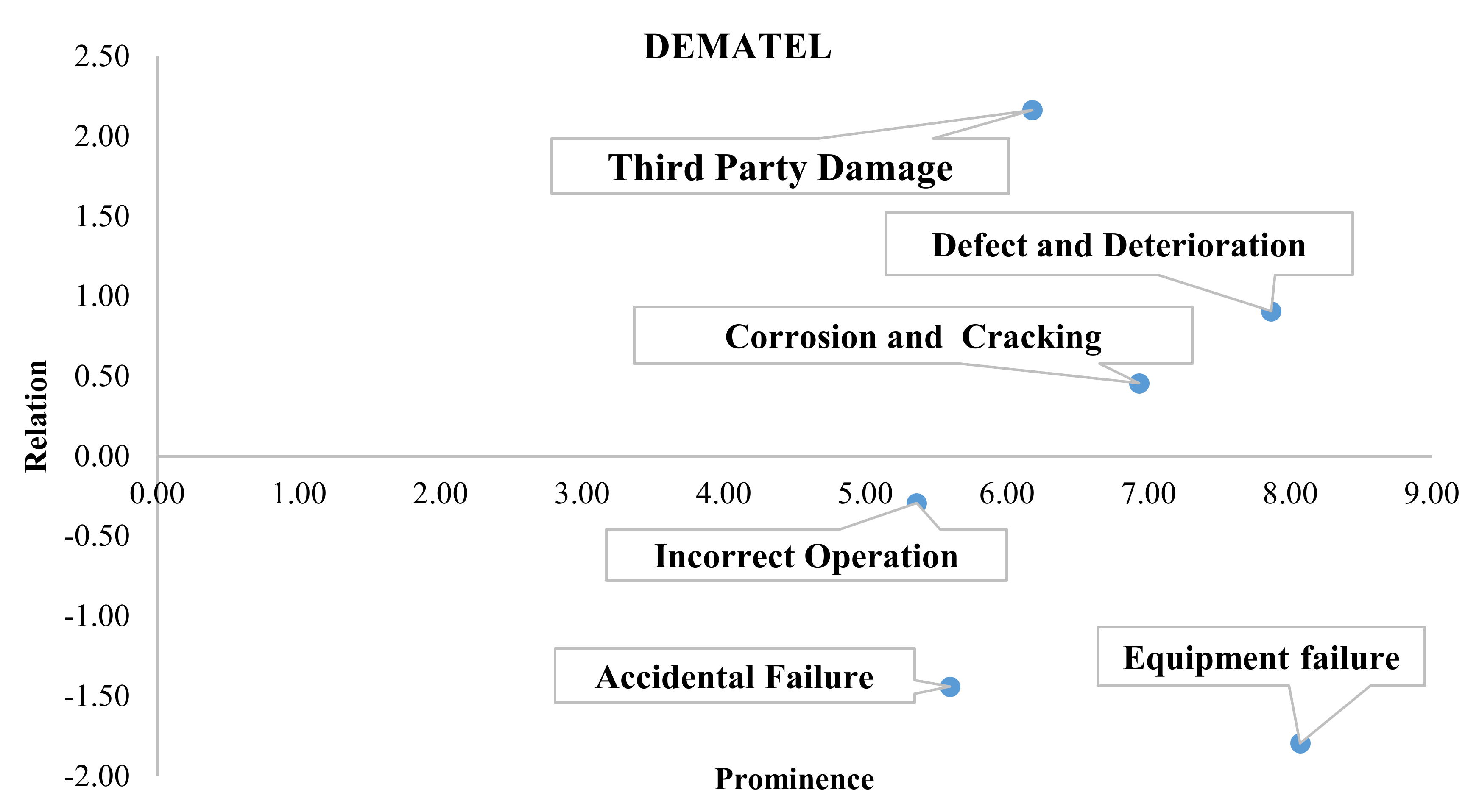
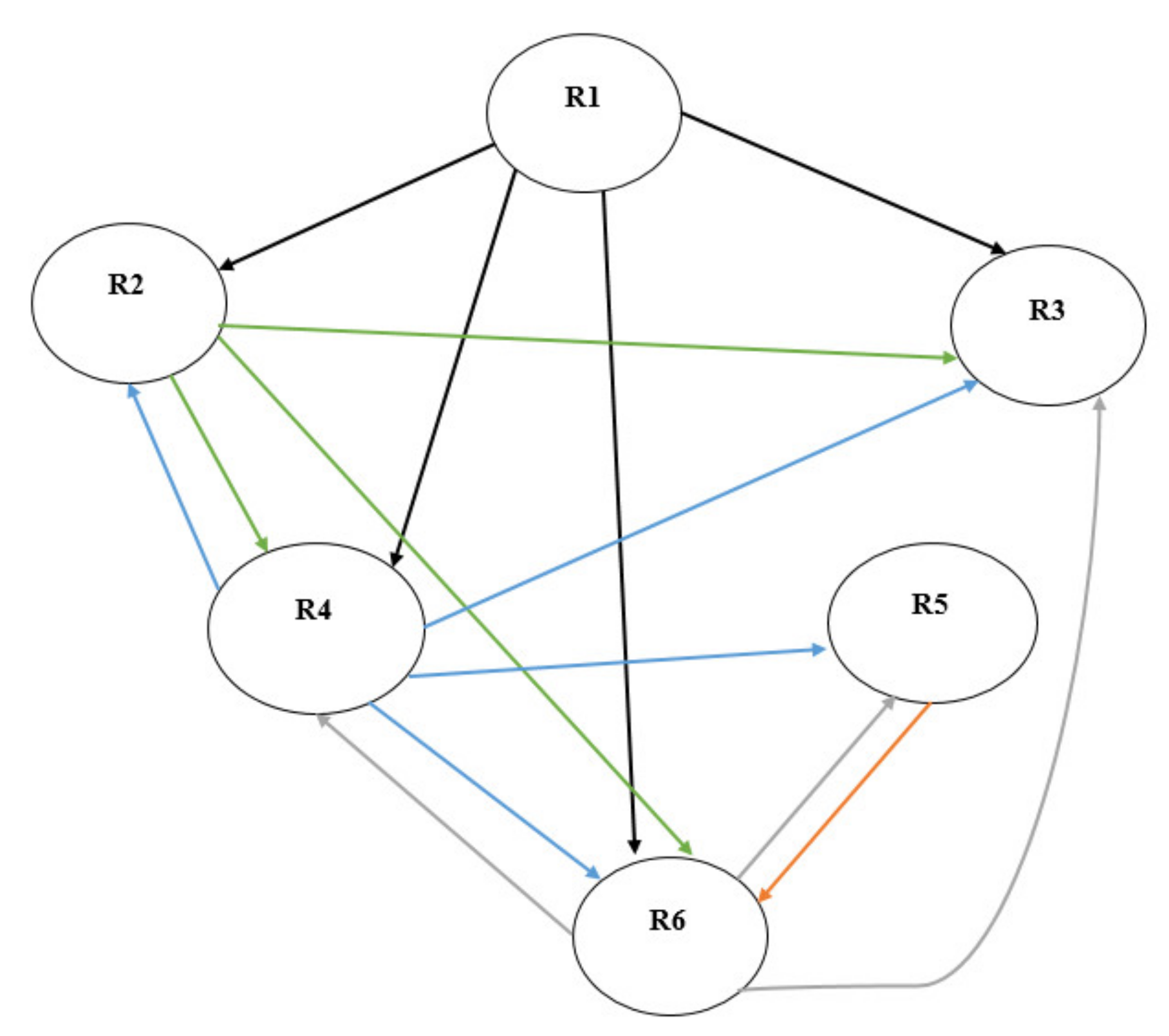
In the DEMATEL, to draw the relationship diagram is followed by the same concept as Rough-DEMATEL. Here also the threshold value is required to develop a causal relationship diagram in (Figure 7). This value is determined by the average matrix (Table 10). In this calculation, the value here is 0.56. In the below (Table 14) average matrix few numerical values are bolded. For example, value compared to (R1) in column and (R2) in row, the value is 0.76 which is bigger than value 0.56. Thereafter, an arrow line will go from (R1) to (R2) likewise the following relationship diagram is being produced (Figure 8) to understand the influence between the causes.
5.4. ISM Calculation
The unit matrix (I) and total relation matrix (T) are added together by using Equation (1) to find out the overall influence matrix (H) (Table 15) in the ISM method.
The basic principle of the reachability set is that it contains its own specific variable, as well as it can help achieve other variables. Then the antecedent set also contains variable of its own and helps other variables for accomplishing. Afterward, the intersection of those mentioned sets is finally computed by all the variables. As a result, the upper-level intersection sets are a similar level in the ISM hierarchy. Thereafter, it will eliminate the rest of the variables [41]. Here Equations (1)–(5) are used to calculate the iterations of the level partitions (Table 16).
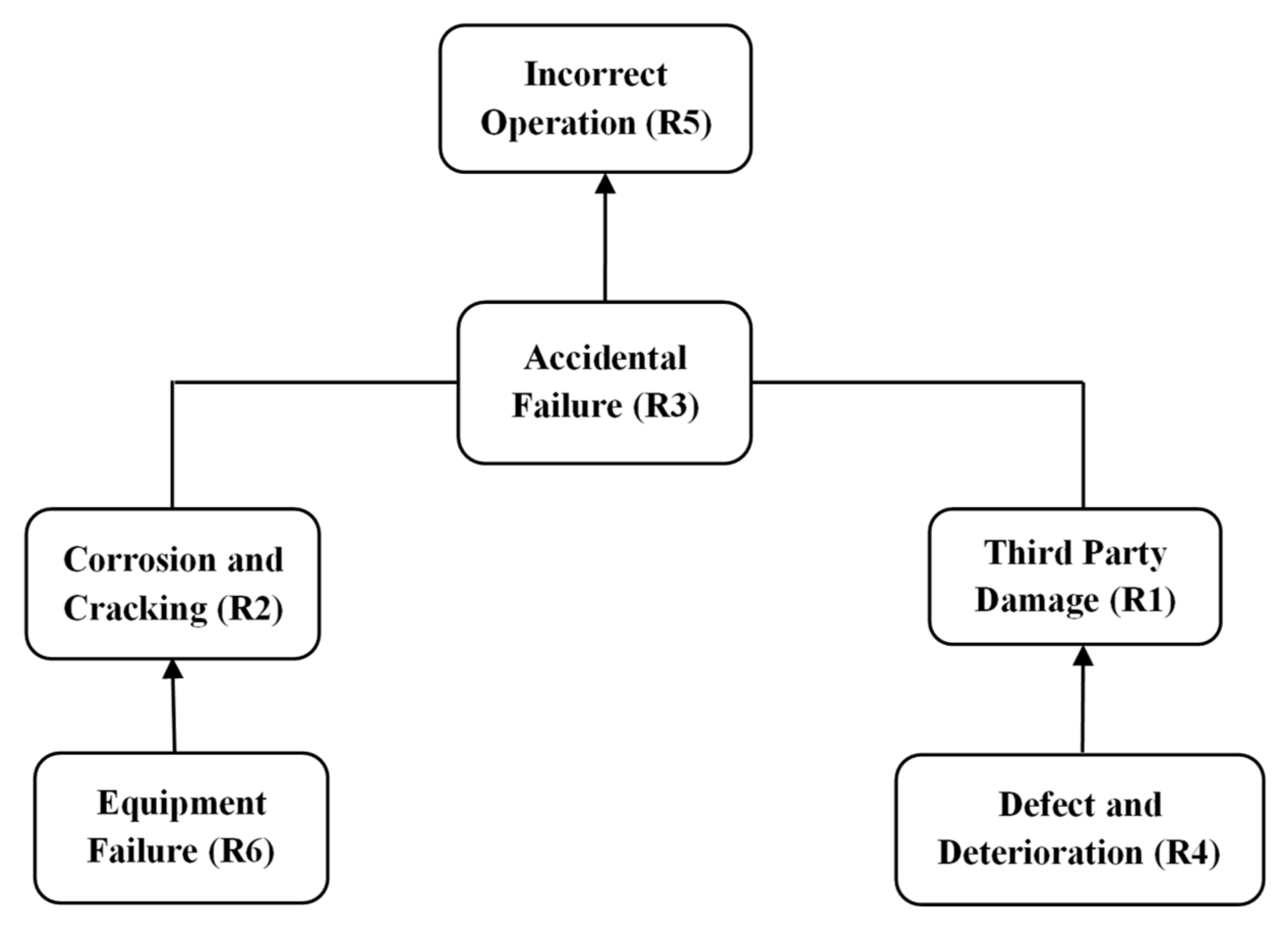
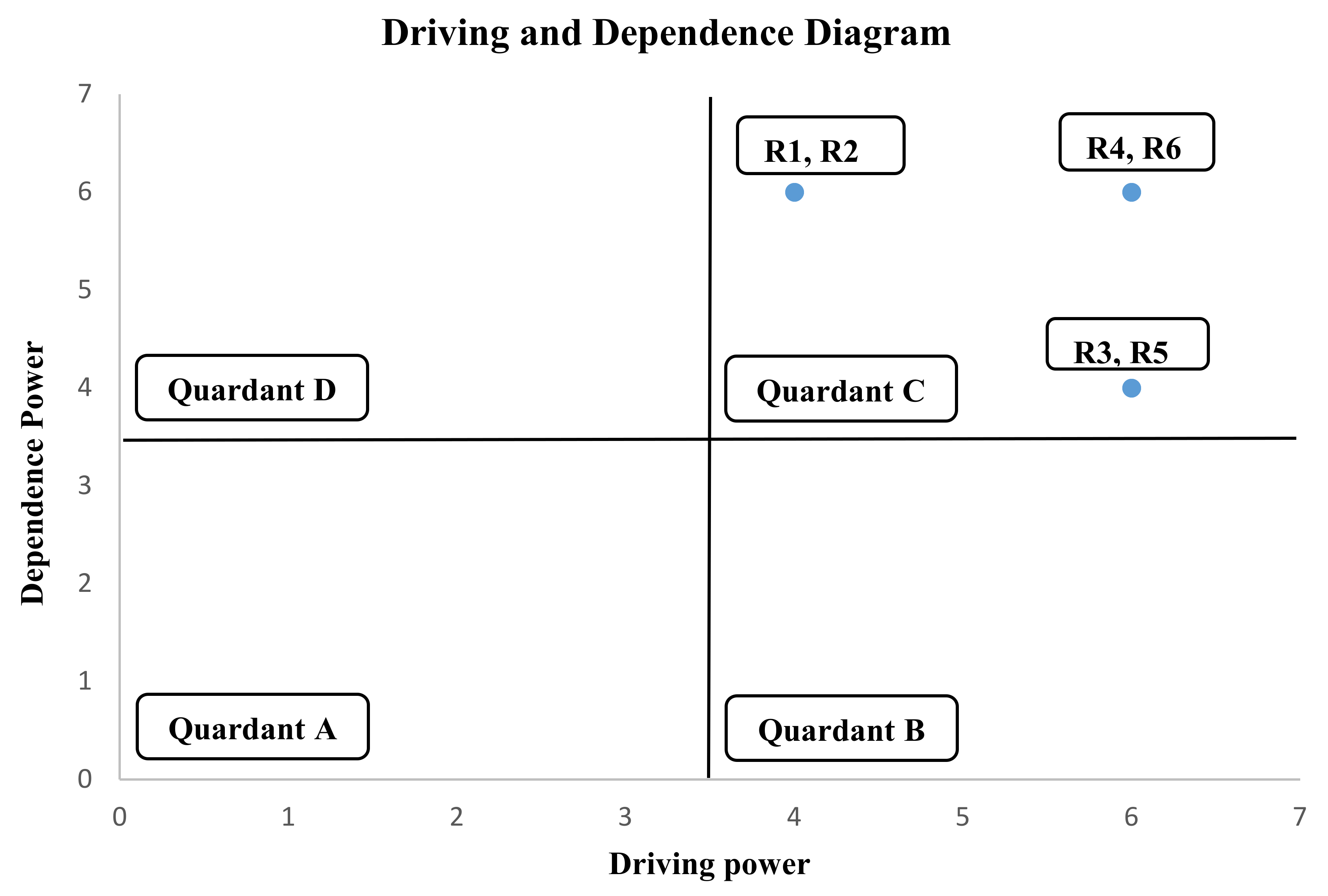
On the completion of the iterations process, the different levels are found such as R5-level I, R3-level II, (R1 and R2) in level III, and (R4 and R6) level IV. Based on this iteration level the final diagraph is drawn (Figure 9). The MICMAC (Figure 10) analysis is calculated based on the driving and dependence power of the transitivity matrix. The MICMAC analysis description is given in the Result and Discussion Section 6.
5.5. Bayesian Belief Network
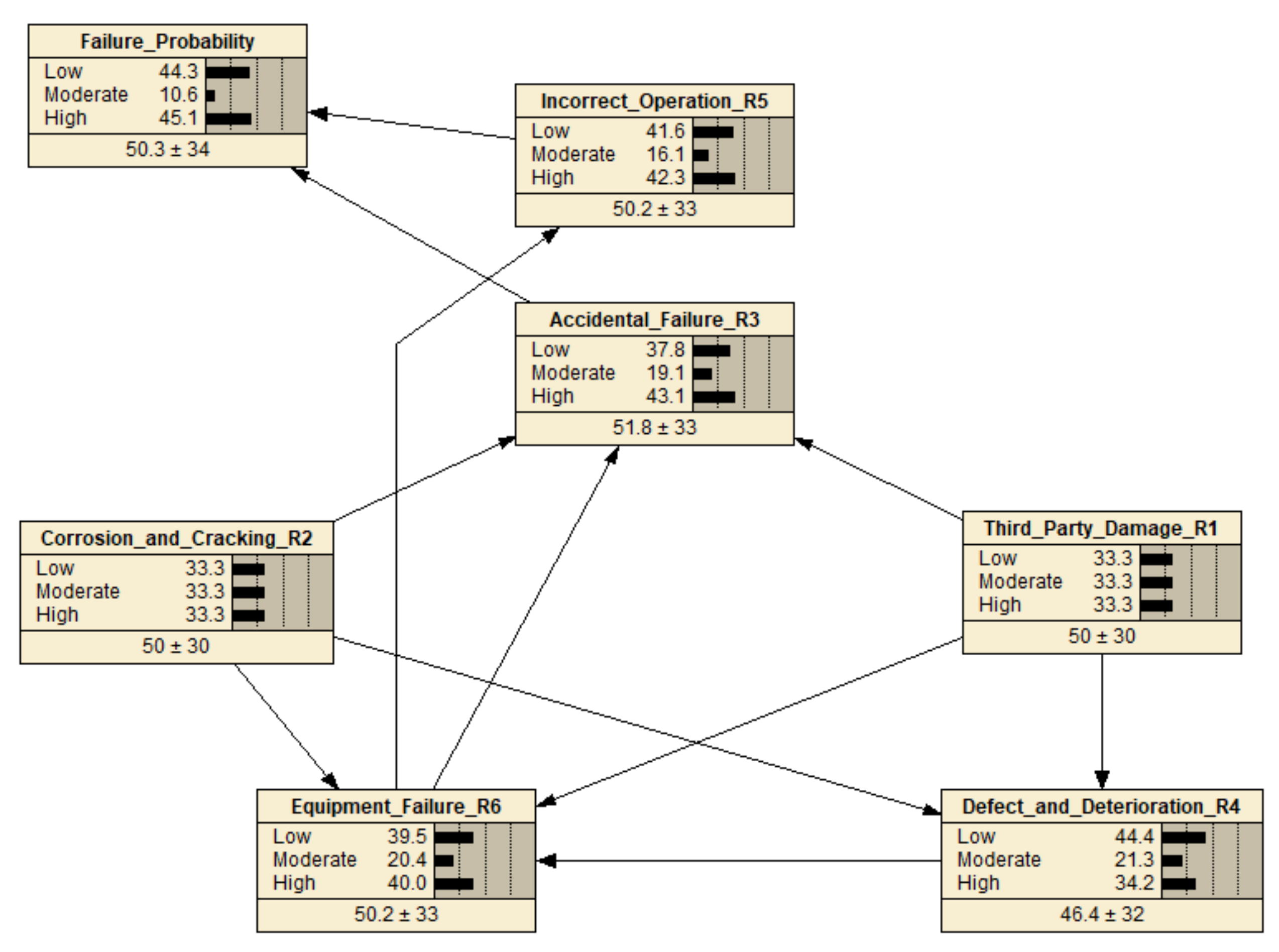
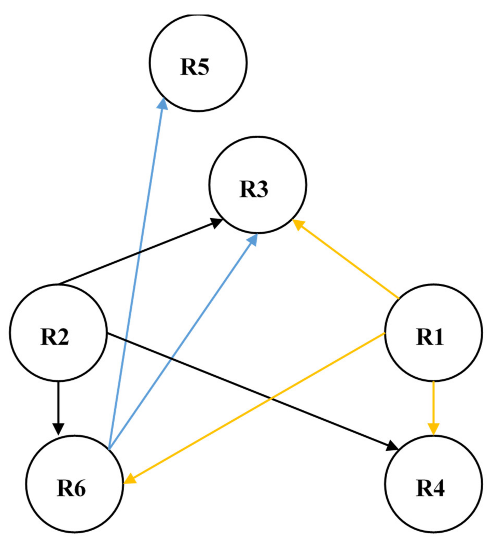
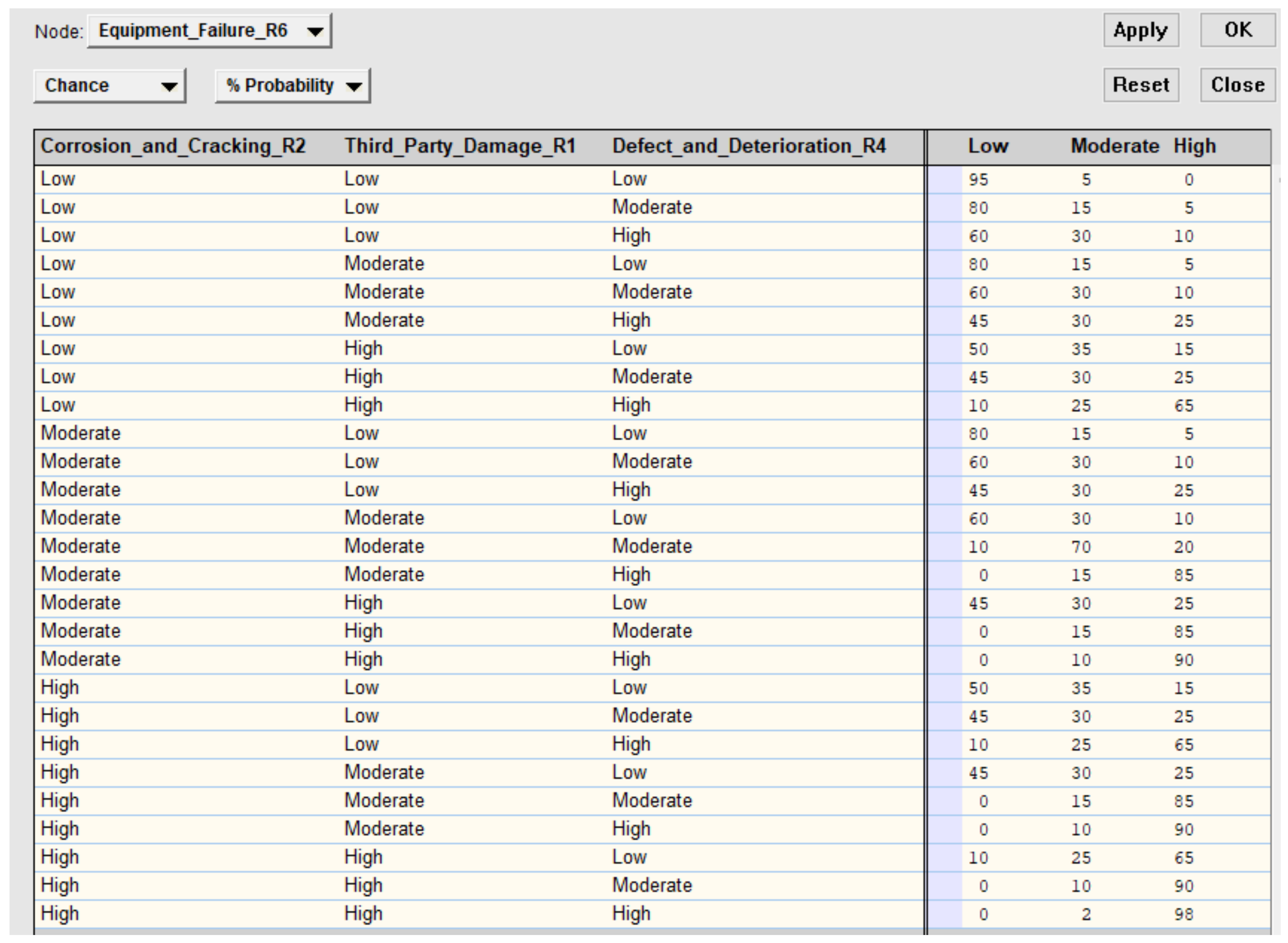
To develop a BBN network, all the loop problems and indirect links need to be withdrawn from the Rough DEMATEL relationship diagram. The compatible revised relationship diagram for the BN model is mentioned in Appendix C, (Figure A1). After elimination of the weaker and circular link from the Rough DEMATEL diagram, the natural gas pipeline failure causes influences among each criterion which are further classified in BBN with the help of such as low medium and high linguistic variable. The experts’ opinions are taken in this entire process. The natural gas failure causes probabilities to influence among all the nodes that are further combined in the Netica software (Figure 11). Table 17 shows two child nodes such as incorrect and accidental failure operation in conditional probabilities Table CPT and the rest of the other causes (CPT) are given in Appendix E.
5.6. Model Validation
In this analysis, the expert’s opinion plays a significant role to develop and validate the BBN model. Besides, extreme condition tests, scenario analysis, and sensitivity analysis also help to validate this model.
5.6.1. Extreme Condition Test
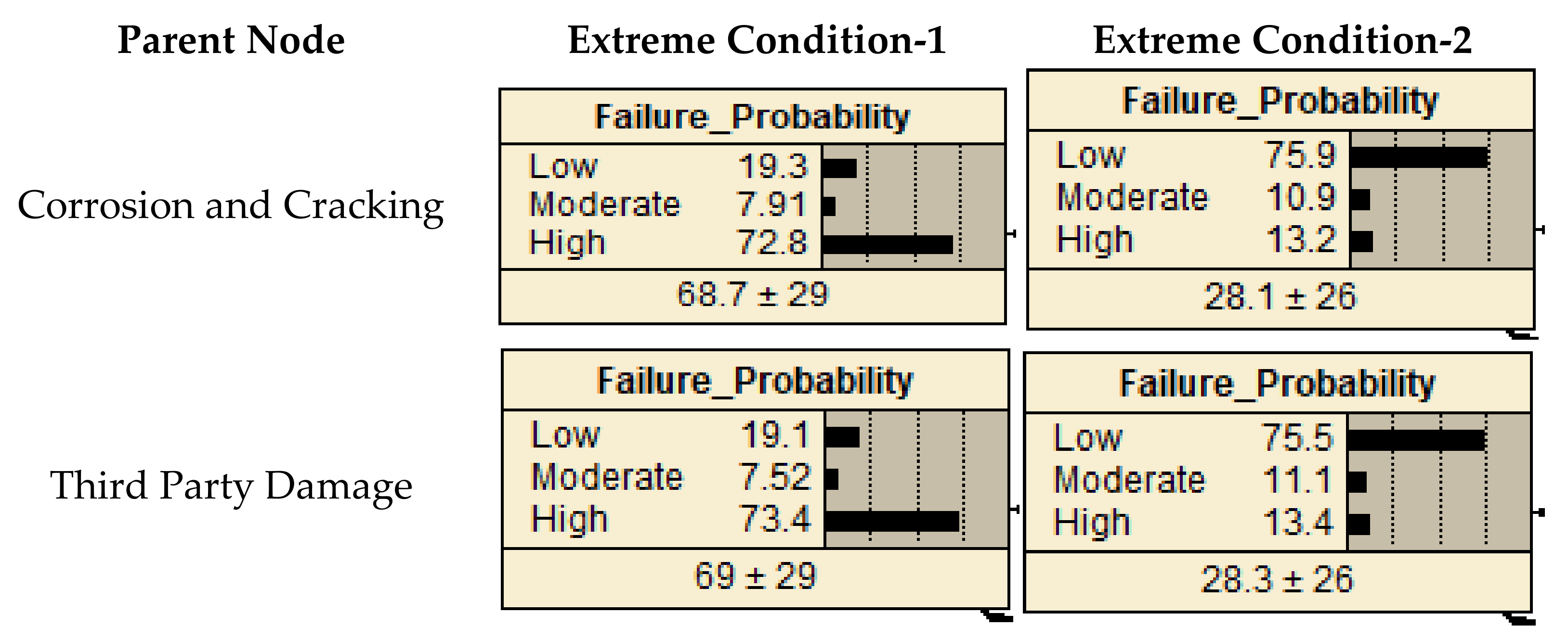
In extreme condition test analysis, two extreme conditions are measured. For instance, the extreme condition case 1 represents that the parent’s node is high, which means the failure probability is high. Oppositely, the extreme condition case 2 signifies that the parent’s node condition is low, which means the failure probability is low. The extreme condition results are shown in Figure 12. In this analysis, three conditions are considered in each node, such as low (0–30), medium (30–70), and high (70–100). Here, Figure 12 shows that while the parent node is corrosion and cracking, then the failure probability is high in extreme condition (1) and low in extreme condition (2) and accordingly 72.8% and 13.2%. Another extreme condition test (failure probability) analysis is conducted because of the parent node third party damage. In this test, the failure probability is high in condition 1 which is 73.4%, whereas low at 13.4% in condition 2.
5.6.2. Scenario Analysis
In this analysis, different scenarios are measured except for the two extreme conditions. The entire analysis is considered based on experts’ opinions. For instance, if parent node corrosion cracking is in moderate states in that case, the failure probability is decreased from high 72.8% to 49.3%. Therefore, if corrosion cracking decreases further from moderate to low then the failure probability decreased further from 49.3% to 13.2%. Here (Figure 12) condition 1 and 2 shows the changes in the three consecutive state.
Another parent node third party damage, whereas the scenario, is almost the same as corrosion and cracking. While the third party is in a moderate state in that case the failure probability is 48.5%. Then the third party decreases more from moderate to low in that case the failure probability is 13.5%. In the same way, the other combination of the child node is also used for model validation.
5.6.3. Sensitivity Analysis
Basically, the most critical parameters in the BBN model are validated with help of sensitivity analysis [51]. Figure 12 shows the fluctuation of failure probability (two extreme conditions test) value in percentage for (Conditions 1 and 2), while the parent node changes between maximum and minimum value. The input parameters value range is accordingly (0–30), (30–70), and (70–100). Here, the variance percentage and reduction are conducted by the support of the parent node to child node such as failure probability. In this analysis the failure causes a probability factor followed by Incorrect Operation 69.8%, Equipment Failure 68.3%, Accidental Failure 63.7%, Defect and Deterioration 48.5%, Corrosion and Cracking 24.1%, and Third-Party Damage 24%. This sensitivity analysis actual reflection of experts’ judgment. As a result, any changes in parent node variance percentage will directly impact the overall failure probability.
6. Results and Discussions
Insufficient amount of data, hidden data patterns, and different professional fields of decision-makers’ opinions are controlled by rough set theory in the decision-making process (Previously discussed in Section 3 under rough set theory). Basically, AHP is integrated with a rough set theory to analyze the rank order. In Rough AHP (Figure 4) distinguish the lower and upper limit values. Finally, the rank order is generated based on differences. In this study, on the basis of all four experts’ combined opinions, the highest three rank orders are accordingly, third party damage, corrosion cracking, and accidental failure. Then defect and deterioration rank order is 4. Thereafter, incorrect operation and equipment failure are holding in the same rank position number 5. Based on Rough AHP, results are finally decided important rank order in total six among ten significant natural gas failure causes criteria.
All those six failures cause criteria are selected (Canadian territory point of view) for the further calculation to analyze the interrelationships and influences. Subsequently, the rest of the six failure criteria are not taken into consideration for the next level of study in this research. Though, those are also important criteria based on an individual country’s perspective.
The Rough DEMATEL method is also integrated with a renowned rough set theory. The key significance between the Rough DEMATEL and normal DEMATEL is the calculation procedure. The main advantage of the Rough DEMATEL method is that it is able to consider the individual judgment for gas pipeline failure, as well as it can do group judgment analysis from all four decision-makers. For an instance, four experts give individual opinion for corrosion and cracking (3,2,3,3), the rough interval upper and lower limit = {(3.00,2.75), (2.75,2.00) (3.00, 2.75), (3.00,2.75)}, then the final average Rough DEMATEL is (2.94, 2.56). Oppositely, the DEMATEL aggregated value is (2.75) only. As a result, Rough DEMATEL is more compatible than normal DEMATEL. This Casual Relationship diagram of Rough DEMATEL (Figure 6) indicates that the above horizontal axis is considered as causes group and below the axis is considered as effects group. The bottom level causes such as incorrect operation, accidental failure, and equipment failure can influence toward the other factors without affecting themselves.
In this Rough DEMATEL study, third party damage is one of the highest important factors as well as defect and deterioration and corrosion cracking. Furthermore, this graphical representation provides the contextual cause-effect relationships, so that the decision-makers can analyze all the critical factors. In summary, of the Rough DEMATEL and DEMATEL, the Rough DEMATEL calculation provides a more precise result than the normal DEMATEL. Consequently, the decision-makers can understand and identify the critical relation and influence the gas pipeline failure criteria. Accordingly, they can take the necessary step to mitigate the pipeline failure of influential causes.
On the basis of driving and dependence power, all the failure causes parameters have been categorized into four significant quadrants, which have already been discussed in Section 3, (3.1.1-MICMAC analysis). To further the failure causes performance analysis, the driving and dependence graphical representation (MICMAC analysis) has been mentioned in (Figure 10). This graphical illustration indicates that the Third-party damage (R1) corrosion cracking (R2), accidental failure (R3), defect and deterioration (R4), incorrect operation (R5), and equipment failure (R6) in quadrant C. Quadrant C means, all the failure causes are linkage variables, which affects the other causes as well as themselves. In this current research no failure criteria are found in quadrant A, quadrant B, and quadrant D.
Thus, it indicates that among the six natural gas pipeline failure causes criteria none of them have both driving and dependence power, low or lower driving and higher dependence power, or higher driving and weak dependency power. The reachability matrix in ISM helps construct the initial diagraph for failure causes analysis (Figure 9). In the next phase, the initial ISM diagraph for variable relationship measures are considered for further modification. Hence, the ISM diagraph for variable relationship is modified further based on three categories as such (i) If the link is weaker between the two causes, it should be withdrawn; (ii) the circular complex link can also be removed; and (iii) if the failure causes are at the same level, it should be withdrawn [52]. Then the modified hierarchical network is combined with BBN.
7. Conclusions
In this study, the “Natural Gas High Transmission Pipeline” failure model development is combined with failure causes analysis. The ultimate aim of this study is to reduce the potential failure risks and prepare for probable hazards. This paper represents different types of hierarchical structures such as Rough AHP, Rough DEMATEL, DEMATEL, ISM, and BBN along with hazardous simulation by using ALOHA software.
Basically, the Rough AHP is a combined method with a well-known rough set theory. The Rough AHP methodology can deal with multiple decision-makers in a vague environment for the decision-making process and recognize the relative importance of each criterion rank order. The Rough DEMATEL method is more compatible with DEMATEL (discussed in the results and discussion section). Then, the modified ISM hierarchical network failure causes a relationship diagram which is combined with BBN to identify the probable influences among the failure criteria. The projected BBN model deals with the influence factors between each failure causes. The integrated method of Rough DEMATEL and ISM analyze the different level of failure dependencies. With the help of Iterations, the failure classification level is analyzed.
The summarization of research contributions are as follows:
- Selecting failure causes from the literature review, open data sources from Canada energy regulatory organization, and industrial/academic experts’ opinions.
- The rough-analytic hierarchy process (Rough-AHP) method is applied for rank order (based on priority) analysis to avoid vagueness of the decision-making process of natural gas pipeline failure causes.
- The casual relationship diagram was developed using both rough-decision making trial and evaluation laboratory (Rough-DEMATEL) and DEMATEL methods. Thereafter, the comparison of these two methods is done to analyze the differences of the results.
- Integrated Rough DEMATEL- ISM methods with BBN to implement and analyze the various interactions for gas pipeline failure causes in accordance with developing the gas pipeline safety and security.
- The MICMAC analysis was developed to analyze the driving and the dependence power of the natural gas transmission pipeline failure causes for the development of gas pipeline system integrity toward the industrial implementation.
Despite these significant studies of failure analysis for natural gas high transmission pipeline, still, present studies have some limitations. First, the failure causes criteria are not fully comprehensive for gas pipeline failure causes analysis. Second, the failure causes criteria may be included or excluded based on countries perspective. Third, the Rough AHP weight calculation results can be compared to other Rough methods such as Rough TOPSIS to evaluate the rank order value. Fourth, the Rough DEMATEL method is unable to distinguish between positive and negative influences. In a future phase of research work, various experts from different fields (related to gas energy) can be added to get a better scenario. These research methodologies can also be implemented in other relevant energy industries to classify the analysis of the potential risks.
Author Contributions
Conceptualization, S.K.A., G.K.; methodology, S.K.A., G.K.; software, S.K.A., G.K.; validation S.K.A., G.K.; formal analysis, S.K.A., G.K.; investigation, S.K.A.; resources, S.K.A., G.K.; data curation, S.K.A.; writing—original draft preparation, S.K.A.; writing—review and editing, S.K.A., G.K.; visualization, S.K.A.; supervision, G.K.; project administration, G.K. All authors have read and agreed to the published version of the manuscript.
Funding
The authors acknowledge the financial support through Natural Science Engineering Research Council, Canada Discovery Grant Program (RGPIN-2019-04704).
Institutional Review Board Statement
Not applicable.
Informed Consent Statement
Informed consent was obtained from all subjects involved in the study.
Data Availability Statement
The sample data collection sheet and the data used for analysis can be available on request to the corresponding author.
Acknowledgments
The authors acknowledge the industry personnel for providing the valuable information and cooperation.
Conflicts of Interest
The authors declare no conflict of interest.
Appendix A. Decision-Maker’s Opinion—Rough AHP

Table A1.
Decision-maker 1.
| Criteria | Engineering Fault | Accidental Failure | Third Party Damage | Human Error | Construction Fault | Natural Force Damage | Corrosion and Cracking | Defect and Deterioration | Incorrect Operation | Equipment Failure |
|---|---|---|---|---|---|---|---|---|---|---|
| Engineering Fault | 1 | 1.00 | 0.50 | 1.00 | 1.00 | 1.00 | 1.00 | 1.00 | 1.00 | 1.00 |
| Accidental Failure | 1.00 | 1 | 0.50 | 1.00 | 1.00 | 1.00 | 0.50 | 0.50 | 1.00 | 1.00 |
| Third Party damage | 2.00 | 2.00 | 1 | 3.00 | 2.00 | 2.00 | 1.00 | 2.00 | 3.00 | 3.00 |
| Human Error | 1.00 | 1.00 | 0.33 | 1 | 1.00 | 1.00 | 0.50 | 0.50 | 1.00 | 1.00 |
| Construction Fault | 1.00 | 1.00 | 0.50 | 1.00 | 1 | 1.00 | 1.00 | 1.00 | 2.00 | 2.00 |
| Natural Force Damage | 1.00 | 1.00 | 0.50 | 1.00 | 1.00 | 1 | 1.00 | 1.00 | 2.00 | 2.00 |
| Corrosion and Cracking | 1.00 | 2.00 | 1.00 | 2.00 | 1.00 | 1.00 | 1 | 2.00 | 3.00 | 3.00 |
| Defect and Destrioraction | 1.00 | 2.00 | 0.50 | 2.00 | 1.00 | 1.00 | 0.50 | 1 | 2.00 | 2.00 |
| Incorrect Operation | 1.00 | 1.00 | 0.33 | 1.00 | 0.50 | 0.50 | 0.33 | 0.50 | 1 | 1.00 |
| Equipment Failure | 1.00 | 1.00 | 0.33 | 1.00 | 0.50 | 0.50 | 0.33 | 0.50 | 1.00 | 1 |
Table A2.
Decision-maker 2.
| Criteria | Engineering Fault | Accidental Failure | Third Party Damage | Human Error | Construction Fault | Natural Force Damage | Corrosion and Cracking | Defect and Deterioration | Incorrect Operation | Equipment Failure |
|---|---|---|---|---|---|---|---|---|---|---|
| Engineering Fault | 1 | 0.50 | 2.00 | 0.50 | 1.00 | 1.00 | 1.00 | 1.00 | 1.00 | 1.00 |
| Accidental Failure | 2.00 | 1 | 4.00 | 1.0 | 2.00 | 1.00 | 2.00 | 2.00 | 1.00 | 1.00 |
| Third Party damage | 0.50 | 0.3 | 1 | 0.25 | 0.50 | 0.25 | 0.50 | 0.50 | 0.25 | 0.25 |
| Human Error | 2.00 | 1.00 | 4.00 | 1 | 2.00 | 1.00 | 2.00 | 2.00 | 1.00 | 1.00 |
| Construction Fault | 1.00 | 0.50 | 2.00 | 0.50 | 1 | 1.00 | 2.00 | 2.00 | 1.00 | 1.00 |
| Natural Force Damage | 1.00 | 1.00 | 4.00 | 1.00 | 1.00 | 1 | 2.00 | 2.00 | 1.00 | 1.00 |
| Corrosion and Cracking | 1.00 | 0.50 | 2.00 | 0.50 | 0.50 | 0.50 | 1 | 1.00 | 0.50 | 0.50 |
| Defect and Destrioraction | 1.00 | 0.50 | 2.00 | 0.50 | 0.50 | 0.50 | 1.00 | 1 | 0.50 | 0.50 |
| Incorrect Operation | 1.00 | 1.00 | 4.00 | 1.00 | 1.00 | 1.00 | 2.00 | 2.00 | 1 | 1.00 |
| Equipment Failure | 1.00 | 1.00 | 4.00 | 1.00 | 1.00 | 1.00 | 2.00 | 2.00 | 1.00 | 1 |
Table A3.
Decision-maker 3.
| Criteria | Engineering Fault | Accidental Failure | Third Party Damage | Human Error | Construction Fault | Natural Force Damage | Corrosion and Cracking | Defect and Deterioration | Incorrect Operation | Equipment Failure |
|---|---|---|---|---|---|---|---|---|---|---|
| Engineering Fault | 1 | 1.0 | 1.0 | 1.0 | 2.0 | 1.0 | 1.0 | 1.0 | 2.0 | 2.0 |
| Accidental Failure | 1.00 | 1 | 2.0 | 2.0 | 2.0 | 2.0 | 2.0 | 1.0 | 2.0 | 2.0 |
| Third Party damage | 1.00 | 0.50 | 1 | 1.0 | 1.0 | 1.0 | 1.0 | 1.0 | 1.0 | 1.0 |
| Human Error | 1.00 | 0.50 | 1.00 | 1 | 1.0 | 1.0 | 1.0 | 1.0 | 1.0 | 1.0 |
| Construction Fault | 0.50 | 0.50 | 1.00 | 1.00 | 1 | 1.0 | 1.0 | 1.0 | 1.0 | 1.0 |
| Natural Force Damage | 1.00 | 0.50 | 1.00 | 1.00 | 1.00 | 1 | 1.0 | 1.0 | 2.0 | 2.0 |
| Corrosion and Cracking | 1.00 | 0.50 | 1.00 | 1.00 | 1.00 | 1.00 | 1 | 1.0 | 2.0 | 2.0 |
| Defect and Destrioraction | 1.00 | 1.00 | 1.00 | 1.00 | 1.00 | 1.00 | 1.0 | 1 | 2.0 | 2.0 |
| Incorrect Operation | 0.50 | 0.50 | 1.00 | 1.00 | 1.00 | 0.50 | 0.5 | 0.50 | 1 | 1.0 |
| Equipment Failure | 0.50 | 0.50 | 1.00 | 1.00 | 1.00 | 0.50 | 0.5 | 0.50 | 1.00 | 1 |
Table A4.
Decision-maker 4.
| Criteria | Engineering Fault | Accidental Failure | Third Party Damage | Human Error | Construction Fault | Natural Force Damage | Corrosion and Cracking | Defect and Deterioration | Incorrect Operation | Equipment Failure |
|---|---|---|---|---|---|---|---|---|---|---|
| Engineering Fault | 1 | 1.00 | 1.00 | 1.00 | 1.00 | 1.00 | 0.50 | 1.00 | 1.00 | 1.00 |
| Accidental Failure | 1.00 | 1 | 0.50 | 1.00 | 1.00 | 1.00 | 0.50 | 1.00 | 1.00 | 1.00 |
| Third Party damage | 1.00 | 2.00 | 1 | 3.00 | 3.00 | 3.00 | 1.0 | 3.00 | 3.00 | 3.00 |
| Human Error | 1.00 | 1.00 | 0.33 | 1 | 1.00 | 1.00 | 0.50 | 1.00 | 1.00 | 1.00 |
| Construction Fault | 1.00 | 1.00 | 0.33 | 1.00 | 1 | 1.00 | 0.50 | 1.00 | 1.00 | 1.00 |
| Natural Force Damage | 1.00 | 1.00 | 0.33 | 1.00 | 1.00 | 1 | 0.50 | 1.00 | 1.00 | 1.00 |
| Corrosion and Cracking | 2.00 | 2.00 | 1.00 | 2.00 | 2.00 | 2.00 | 1 | 3.00 | 3.00 | 3.00 |
| Defect and Destrioraction | 1.00 | 1.00 | 0.33 | 1.00 | 1.00 | 1.00 | 0.33 | 1 | 1.00 | 1.00 |
| Incorrect Operation | 1.00 | 1.00 | 0.33 | 1.00 | 1.00 | 1.00 | 0.33 | 1.00 | 1 | 1.00 |
| Equipment Failure | 1.00 | 1.00 | 0.33 | 1.00 | 1.00 | 1.00 | 0.33 | 1.00 | 1.00 | 1 |
Appendix B. Rough AHP
Appendix C. Relationship Diagram
Figure A1.
Modified hierarchical network.

Appendix D. Decision-Makers Opinion—Rough DEMATEL
Table A5.
Decision-maker 1.
| Criteria | Third Party Damage | Corrosion and Cracking | Accidental Failure | Defects and Deterioration | Incorrect Operation | Equipment Failure |
|---|---|---|---|---|---|---|
| Third Party Damage | 0 | 3 | 1 | 4 | 1 | 3 |
| Corrosion and Cracking | 4 | 0 | 3 | 4 | 0 | 3 |
| Accidental Failure | 0 | 0 | 0 | 0 | 0 | 4 |
| Defects and Deterioration | 4 | 4 | 3 | 0 | 0 | 3 |
| Incorrect Operation | 0 | 2 | 3 | 2 | 0 | 3 |
| Equipment Failure | 0 | 1 | 3 | 3 | 4 | 0 |
Table A6.
Decision-maker 2.
| Criteria | Third Party Damage | Corrosion and Cracking | Accidental Failure | Defects and Deterioration | Incorrect Operation | Equipment Failure |
|---|---|---|---|---|---|---|
| Third Party Damage | 0 | 2 | 0 | 0 | 0 | 1 |
| Corrosion and Cracking | 0 | 0 | 0 | 1 | 2 | |
| Accidental Failure | 0 | 0 | 0 | 0 | 0 | 0 |
| Defects and Deterioration | 0 | 2 | 1 | 0 | 4 | 3 |
| Incorrect Operation | 0 | 0 | 0 | 0 | 0 | 3 |
| Equipment Failure | 0 | 0 | 0 | 1 | 2 | 0 |
Table A7.
Decision-maker 3.
| Criteria | Third Party Damage | Corrosion and Cracking | Accidental Failure | Defects and Deterioration | Incorrect Operation | Equipment Failure |
|---|---|---|---|---|---|---|
| Third Party Damage | 0 | 3 | 4 | 4 | 1 | 1 |
| Corrosion and Cracking | 0 | 0 | 2 | 3 | 1 | 3 |
| Accidental Failure | 2 | 2 | 0 | 0 | 1 | 3 |
| Defects and Deterioration | 3 | 3 | 0 | 0 | 0 | 3 |
| Incorrect Operation | 0 | 1 | 2 | 0 | 0 | 3 |
| Equipment Failure | 0 | 1 | 3 | 3 | 3 | 0 |
Table A8.
Decision-maker 4.
| Criteria | Third Party Damage | Corrosion and Cracking | Accidental Failure | Defects and Deterioration | Incorrect Operation | Equipment Failure |
|---|---|---|---|---|---|---|
| Third Party Damage | 0 | 3 | 4 | 4 | 1 | 2 |
| Corrosion and Cracking | 2 | 0 | 2 | 3 | 1 | 3 |
| Accidental Failure | 2 | 2 | 0 | 0 | 2 | 3 |
| Defects and Deterioration | 3 | 4 | 0 | 0 | 0 | 4 |
| Incorrect Operation | 0 | 1 | 2 | 2 | 0 | 3 |
| Equipment Failure | 0 | 1 | 3 | 3 | 3 | 0 |
Appendix E. CPT Figures of Failure
Figure A2.
Conditional probabilities table (CPT) for equipment failure.

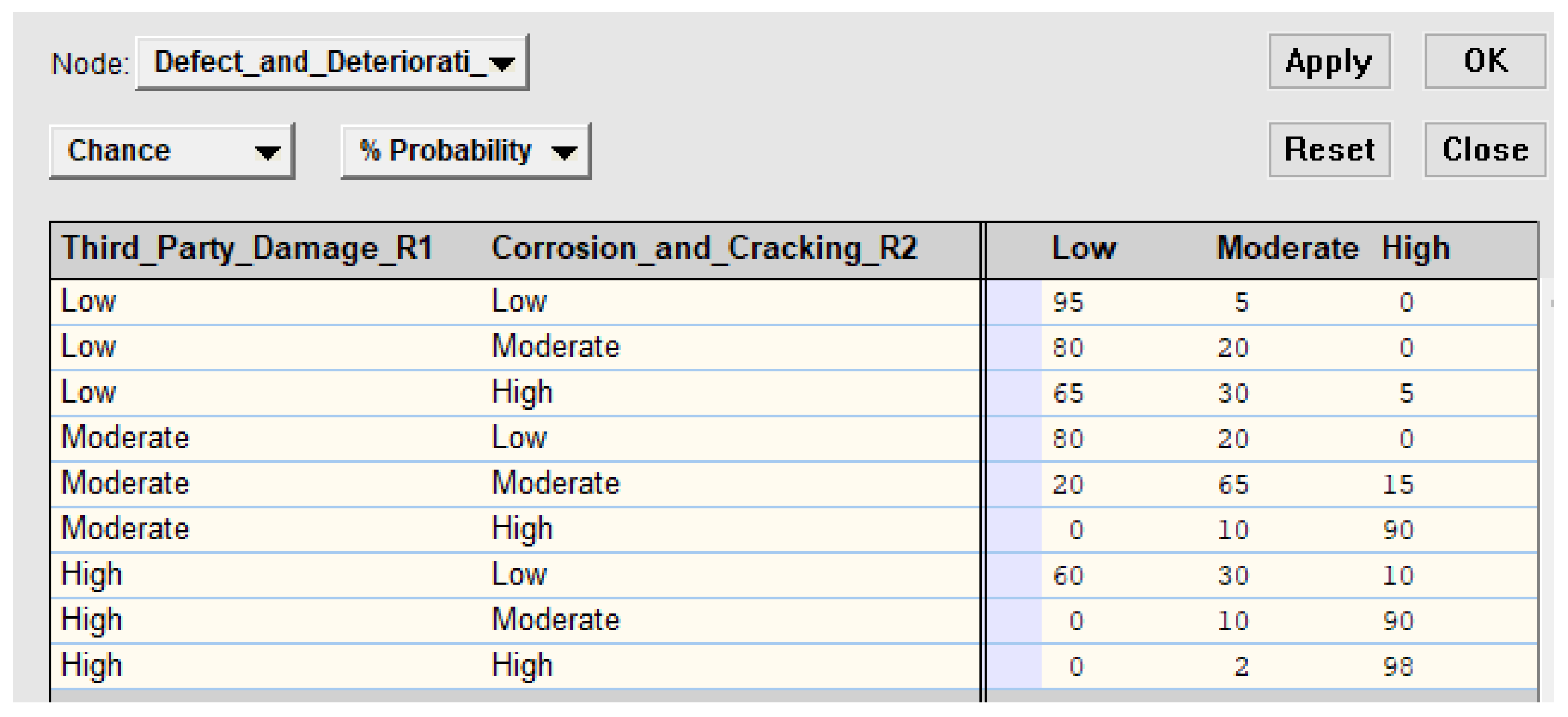
Figure A3.
Conditional probabilities table (CPT) for defect and deterioration.

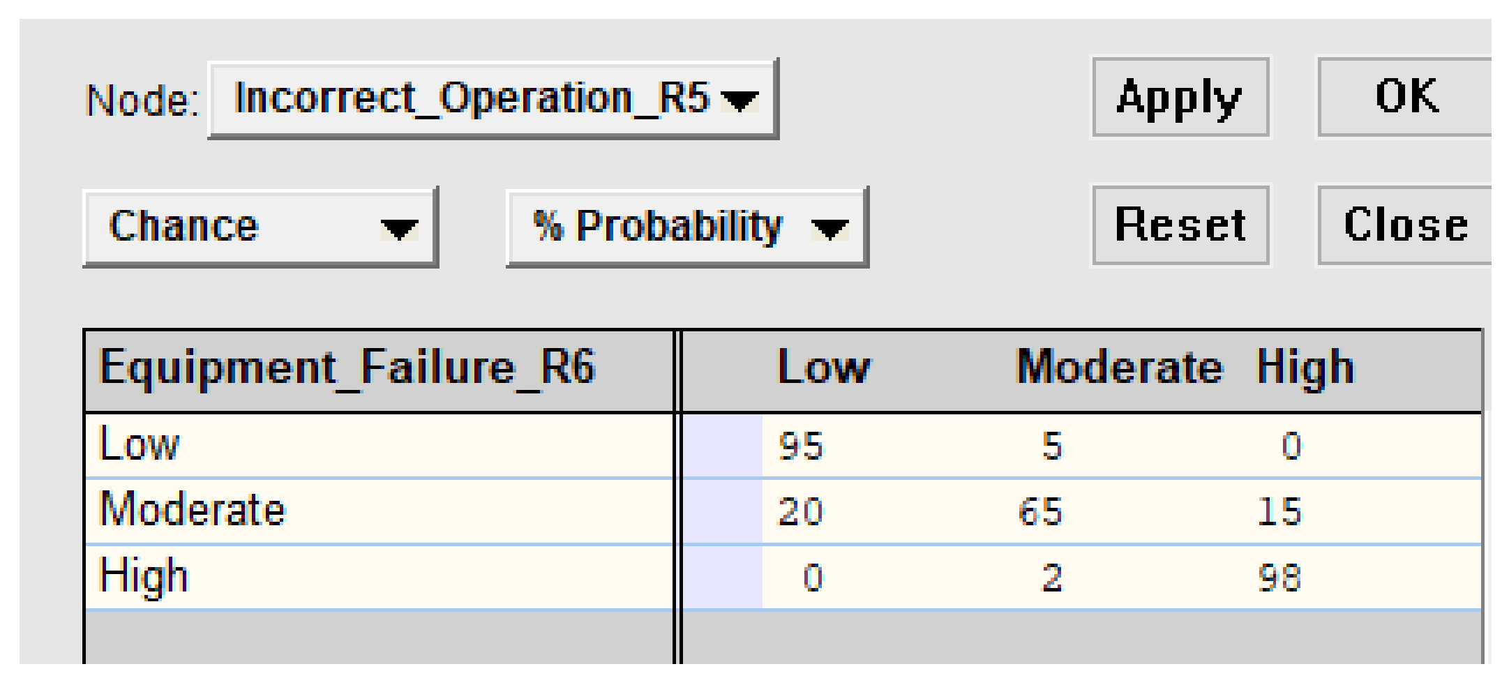
Figure A4.
Conditional probabilities table (CPT) for incorrect operation.

References
- The Canadian Association of Petroleum Producers. Canada’s Natural Gas; CAPP: Calgary, AB, Canada, 2019; pp. 1–56. [Google Scholar]
- Canada Energy Regulator. Pipeline Regulation in Canada. Available online: https://www.cer-rec.gc.ca/en/about/who-we-are-what-we-do/pipeline-regulation-in-canada.html (accessed on 5 October 2020).
- Santarelli, J.S. Risk Analysis of Natural Gas Distribution Pipelines with Respect to Third Party Damage. Master’s Thesis, The University of Western Ontario, London, ON, Canada, 25 April 2019. [Google Scholar]
- Belvederesi, C.; Thompson, M.S.; Komers, P.E. Canada’s federal database is inadequate for the assessment of environmental consequences of oil and gas pipeline failures. Environ. Rev. 2017, 25, 415–422. [Google Scholar] [CrossRef] [Green Version]
- Chen, X.; Wu, Z.; Chen, W.; Kang, R.; He, X.; Miao, Y. Selection of key indicators for reputation loss in oil and gas pipeline failure event. Eng. Fail. Anal. 2019, 99, 69–84. [Google Scholar] [CrossRef]
- Hao, Y.; Yang, W.; Xing, Z.; Yang, K.; Sheng, L.; Yang, J. Calculation of accident probability of gas pipeline based on evolutionary tree and moment multiplication. Int. J. Press. Vessel. Pip. 2019, 176, 103955. [Google Scholar] [CrossRef]
- Wang, X.; Duan, Q. Improved AHP–TOPSIS model for the comprehensive risk evaluation of oil and gas pipelines. Pet. Sci. 2019, 16, 1479–1492. [Google Scholar] [CrossRef] [Green Version]
- Li, F.; Wang, W.; Dubljevic, S.; Khan, F.; Xu, J.; Yi, J. Analysis on accident-causing factors of urban buried gas pipeline network by combining DEMATEL, ISM and BN methods. J. Loss Prev. Process Ind. 2019, 61, 49–57. [Google Scholar] [CrossRef]
- Shan, X.; Liu, K.; Sun, P.-L. Risk analysis on leakage failure of natural gas pipelines by fuzzy bayesian network with a bow-tie model. Sci. Program. 2017, 2017, 1–11. [Google Scholar] [CrossRef] [Green Version]
- Dai, L.; Wang, D.-P.; Wang, T.; Feng, Q.; Yang, X. Analysis and comparison of long-distance pipeline failures. J. Pet. Eng. 2017, 2017, 1–7. [Google Scholar] [CrossRef] [Green Version]
- Witek, M. Gas transmission pipeline failure probability estimation and defect repairs activities based on in-line inspection data. Eng. Fail. Anal. 2016, 70, 255–272. [Google Scholar] [CrossRef]
- Li, J.; Zhang, H.; Han, Y.; Wang, B. Study on failure of third-party damage for urban gas pipeline based on fuzzy comprehensive evaluation. PLoS ONE 2016, 11, e0166472. [Google Scholar] [CrossRef]
- EGIG. 10th Report of the European Gas Pipeline Incident Data Group. Available online: https://www.egig.eu/reports (accessed on 5 October 2020).
- Global News. Woman Charged with Impaired Driving after Car Crashes into London, Ont. House Causing Large Explosion. Available online: https://globalnews.ca/news/5768211/gas-house-explosion-london-ontario/ (accessed on 2 October 2020).
- Metwally, K.G.; Hussein, M.M.; Akl, A.Y. Structural deterioration of pipelines and its impact on ground surface. J. Eng. Appl. Sci. 2009, 56, 361–380. [Google Scholar]
- U.S. Department of Transportation—Pipeline and Hazardous Materials Safety Administration. Evaluating the Stability of Manufacturing and Construction Defects in Natural Gas Pipelines. Available online: https://www.phmsa.dot.gov/pipeline/gas-transmission-integrity-management/evaluating-stability-manufacturing-and-construction-defects-in-natural-gas-pipelines (accessed on 4 October 2020).
- Selvik, J.T.; Bellamy, L.J. Addressing human error when collecting failure cause information in the oil and gas industry: A review of ISO 14224:2016. Reliab. Eng. Syst. Saf. 2020, 194, 106418. [Google Scholar] [CrossRef]
- Šarkoćević, Ž.; Lazarević, D.; Čamagić, I.; Radojković, M.; Stojčetović, B. The pipeline defect assessment manual—Short review. In Proceedings of the XXI YUCORR International Conference, Tara Mountain, Serbia, 17–20 September 2009; pp. 161–166. [Google Scholar]
- Černý, I.; Mikulová, D.; Sís, J. Examples of actual defects in high pressure pipelines and probabilistic assessment of residual life for different types of pipeline steels. Procedia Struct. Integr. 2017, 7, 431–437. [Google Scholar] [CrossRef]
- Stević, Ž.; Tanackov, I.; Vasiljević, M.; Rikalović, A. Supplier evaluation criteria: AHP rough approach. In Proceedings of the XVII International Scientific Conference on Industrial Systems (IS’17), Novi Sad, Serbia, 4–6 October 2017; pp. 298–303. [Google Scholar]
- Fazlollahtabar, H.; Vasiljević, M.; Stević, Ž.; Vesković, S. Evaluation of supplier criteria in automotive industry using rough AHP. In Proceedings of the 1st International Conference on Management, Engineering and Environment ICMNEE, Belgrade, Serbia, 3–4 October 2019; pp. 186–197. [Google Scholar]
- Fakhravar, D.; Khakzad, N.; Reniers, G.; Cozzani, V. Security vulnerability assessment of gas pipelines using Discrete-time Bayesian network. Process Saf. Environ. Prot. 2017, 111, 714–725. [Google Scholar] [CrossRef]
- Sajid, Z.; Khan, F.; Zhang, Y. Integration of interpretive structural modelling with Bayesian network for biodiesel performance analysis. Renew. Energy 2017, 107, 194–203. [Google Scholar] [CrossRef]
- Francis, R.A.; Guikema, S.D.; Henneman, L. Bayesian Belief Networks for predicting drinking water distribution system pipe breaks. Reliab. Eng. Syst. Saf. 2014, 130, 1–11. [Google Scholar] [CrossRef]
- Beaudequin, D.; Harden, F.; Roiko, A.; Mengersen, K. Utility of Bayesian networks in QMRA-based evaluation of risk reduction options for recycled water. Sci. Total Environ. 2016, 541, 1393–1409. [Google Scholar] [CrossRef]
- Duan, R.-X.; Zhou, H.-L. A new fault diagnosis method based on fault tree and Bayesian Networks. Energy Procedia 2012, 17, 1376–1382. [Google Scholar] [CrossRef] [Green Version]
- Lin, Y.T.; Lin, C.L.; Yu, H.C.; Tzeng, G.H. Utilisation of interpretive structural modelling method in the analysis of interrelationship of vendor performance factors. Int. J. Bus. Perform. Manag. 2011, 12, 260. [Google Scholar] [CrossRef]
- Altuntas, S.; Dereli, T. A novel approach based on DEMATEL method and patent citation analysis for prioritizing a portfolio of investment projects. Expert Syst. Appl. 2015, 42, 1003–1012. [Google Scholar] [CrossRef]
- Gandhi, S.; Mangla, S.K.; Kumar, P.; Kumar, D. Evaluating factors in implementation of successful green supply chain management using DEMATEL: A case study. Int. Strat. Manag. Rev. 2015, 3, 96–109. [Google Scholar] [CrossRef] [Green Version]
- Ilieva, G. Group decision analysis with interval type-2 fuzzy numbers. Cybern. Inf. Technol. 2017, 17, 31–44. [Google Scholar] [CrossRef] [Green Version]
- Chang, B.; Chang, C.-W.; Wu, C.-H. Fuzzy DEMATEL method for developing supplier selection criteria. Expert Syst. Appl. 2011, 38, 1850–1858. [Google Scholar] [CrossRef]
- Song, W.; Cao, J. A rough DEMATEL-based approach for evaluating interaction between requirements of product-service system. Comput. Ind. Eng. 2017, 110, 353–363. [Google Scholar] [CrossRef]
- Khoo, L.-P.; Zhai, L.-Y. A prototype genetic algorithm-enhanced rough set-based rule induction system. Comput. Ind. 2001, 46, 95–106. [Google Scholar] [CrossRef]
- Song, W.; Ming, X.; Wu, Z. An integrated rough number-based approach to design concept evaluation under subjective environments. J. Eng. Des. 2013, 24, 320–341. [Google Scholar] [CrossRef]
- Warfield, J.N. Implication structures for system interconnection matrices. IEEE Trans. Syst. Man Cybern. 1976, 6, 18–24. [Google Scholar] [CrossRef]
- Vinodh, S.; Ramesh, K.; Arun, C.S. Application of interpretive structural modelling for analysing the factors influencing integrated lean sustainable system. Clean Technol. Environ. Policy 2016, 18, 413–428. [Google Scholar] [CrossRef]
- Warfield, J.N. Developing interconnection matrices in structural modeling. IEEE Trans. Syst. Man Cybern. 1974, 4, 81–87. [Google Scholar] [CrossRef] [Green Version]
- Sage, A.P. Methodology for Large-Scale Systems; McGraw-Hill: New York, NY, USA, 1977; p. 458. [Google Scholar]
- Sharma, R.; Garg, S. Interpretive structural modelling of enablers for improving the performance of automobile service centre. Int. J. Serv. Oper. Inform. 2010, 5, 351. [Google Scholar] [CrossRef]
- Thakkar, J.; Deshmukh, S.; Gupta, A.D.; Shankar, R. Development of a balanced scorecard. Int. J. Prod. Perform. Manag. 2006, 56, 25–59. [Google Scholar] [CrossRef]
- Azevedo, S.G.; Carvalho, H.; Machado, V.C. Using interpretive structural modelling to identify and rank performance measures. Balt. J. Manag. 2013, 8, 208–230. [Google Scholar] [CrossRef]
- Yu, W.; Song, S.; Li, Y.; Min, Y.; Huang, W.; Wen, K.; Gong, J. Gas supply reliability assessment of natural gas transmission pipeline systems. Energy 2018, 162, 853–870. [Google Scholar] [CrossRef]
- Dundulis, G.; Žutautaitė, I.; Janulionis, R.; Ušpuras, E.; Rimkevičius, S.; Eid, M. Integrated failure probability estimation based on structural integrity analysis and failure data: Natural gas pipeline case. Reliab. Eng. Syst. Saf. 2016, 156, 195–202. [Google Scholar] [CrossRef]
- Sushil. Incorporating polarity of relationships in ISM and TISM for theory building in information and organization management. Int. J. Inf. Manag. 2018, 43, 38–51. [Google Scholar] [CrossRef]
- Wu, H.-H.; Chang, S.-Y. A case study of using DEMATEL method to identify critical factors in green supply chain management. Appl. Math. Comput. 2015, 256, 394–403. [Google Scholar] [CrossRef]
- Song, W.; Ming, X.; Wu, Z.; Zhu, B. A rough TOPSIS approach for failure mode and effects analysis in uncertain environments. Qual. Reliab. Eng. Int. 2013, 30, 473–486. [Google Scholar] [CrossRef]
- Zhai, L.-Y.; Khoo, L.P.; Zhong, Z.-W. A rough set enhanced fuzzy approach to quality function deployment. Int. J. Adv. Manuf. Technol. 2008, 37, 613–624. [Google Scholar] [CrossRef]
- Zhu, G.-N.; Hu, J.; Qi, J.; Gu, C.-C.; Peng, Y.-H. An integrated AHP and VIKOR for design concept evaluation based on rough number. Adv. Eng. Inform. 2015, 29, 408–418. [Google Scholar] [CrossRef]
- Saaty, T.L.; Vargas, L.G. Models, Methods, Concepts & Applications of the Analytic Hierarchy Process, 2nd ed.; Springer Science & Business Media: New York, NY, USA, 2012; p. XIV-346. [Google Scholar]
- Vasiljević, M.; Fazlollahtabar, H.; Stević, Ž.; Vesković, S. A rough multicriteria approach for evaluation of the supplier criteria in automotive industry. Decis. Mak. Appl. Manag. Eng. 2018, 1, 82–96. [Google Scholar] [CrossRef]
- Kabir, G.; Balek, N.B.C.; Tesfamariam, S. Consequence-based framework for buried infrastructure systems: A Bayesian belief network model. Reliab. Eng. Syst. Saf. 2018, 180, 290–301. [Google Scholar] [CrossRef]
- Nadkarni, S.; Shenoy, P.P. A causal mapping approach to constructing Bayesian networks. Decis. Support Syst. 2004, 38, 259–281. [Google Scholar] [CrossRef] [Green Version]
Figure 1.
Natural gas pipeline failure root cause analysis.

Figure 2.
The rough set theory basic notions (Reproduced after Stević et al., 2017a) [20].
Figure 2.
The rough set theory basic notions (Reproduced after Stević et al., 2017a) [20].

Figure 3.
Integrated multi-criteria decision analysis (MCDA) method with Bayesian Belief Network (BBN) for failure analysis framework.
Figure 3.
Integrated multi-criteria decision analysis (MCDA) method with Bayesian Belief Network (BBN) for failure analysis framework.

Figure 4.
Weights of Rough analytic hierarchy process (AHP) for natural gas pipeline failure causes.
Figure 4.
Weights of Rough analytic hierarchy process (AHP) for natural gas pipeline failure causes.

Figure 5.
Causal relationship diagram of Rough-DEMATEL.

Figure 6.
Rough-DEMATEL relationship diagram.

Figure 7.
Casual relationship diagram of DEMATEL.

Figure 8.
DEMATEL relationship diagram.

Figure 9.
The final ISM diagraph for variable relationship measures.

Figure 10.
MICMAC analysis of natural gas pipeline failure causes.

Figure 11.
The failure causes influences probabilities are combined in BBN.

Figure 12.
Failure probability extreme condition test for BBN model.

Table 1.
Summary of the gas pipeline failure causes.
| References | Criteria | Key Points |
|---|---|---|
| (Chen et al., 2019), (J. Li, Zhang, Han, & Wang, 2016), (Santarelli, 2019) [3,5,12] | The Third-Party Damage | Unauthorized third party constructions and Dig by heavy machinery without informing the natural gas provider authority. |
| (Chen et al., 2019), (European Gas Pipeline Incident Data Group (EGIG), 2018) [5,13] | Corrosion and Cracking | Metal loss, reduce the thickness, develop the crack, and external and internal corrosion. |
| (Rodrigues et al., 2019), (Shan, Liu, & Sun, 2017), (Canada Energy Regulator, 2019) [2,9,14] | Accidental Failure (Proposed) | Fire explosion, ignition with substantial casualties, and nearby industry fire explosion. |
| (Metwally et al., 2009), (Barrett, 2007) [15,16] | Defect and Deterioration | Structural deterioration in the aging pipe and decreases the load-bearing capacity (i.e., pressure flow, internal and external load). |
| (Dai et al., 2017) (Hao et al., 2019) [6,10] | Incorrect Operation | Opening a wrong valve, over pressuring on particular equipment, mechanical pressure relief system, and incorrectly assessing a condition during excavation work. |
| (European Gas Pipeline Incident Data Group (EGIG), 2018) (Dai et al., 2017) [10,13] | Equipment Failure | Malfunction of natural gas pipeline valves, tanks, meters, pumps, compressors, and other components and devices. |
| (European Gas Pipeline Incident Data Group (EGIG), 2018), (Selvik & Bellamy, 2020) [13,17] | Human Error | Inappropriate maintenance practice, bolts are not tightening properly, lack of frequent inspections, inappropriate operation practices, unsafe acts, operators’ mistakes in action planning, improper use of equipment, and error in documentation, etc. |
| (Dai et al., 2017), (Hao et al., 2019), (European Gas Pipeline Incident Data Group (EGIG), 2018) [6,10,13] | Natural Force Damage | Earth movement, earthquake, heavy rain/flood, lightning, frost heave. |
| (Camagic & Stojcetovic, 2019) (Černý, Mikulová, & Sís, 2017) [18,19] | Engineering Fault (Proposed) | Defects of design, fabrication and manufacturing, inadequate pipeline load pressure calculation. |
| (Barrett, 2007), (Chen et al., 2019), (Dai et al., 2017), (European Gas Pipeline Incident Data Group (EGIG), 2018) [5,10,13,16] | Construction Fault | Girth weld defects, spiral weld defects, gouges and dents, improper backfill, wrinkle coupling failures, inappropriate construction practices, and incorrect markers. |
Table 2.
Summary of the gas pipeline failure causes analysis methods.
| References | Key Methodology | Application Area |
|---|---|---|
| (Li et al., 2019) [8] | DEMATEL, ISM, Bayesian network (BN) | Urban buried gas pipeline failure analysis |
| (Wang & Duan, 2019) [7] | Improved AHP, Improved TOPSIS | Oil and Gas pipeline failure analysis |
| (Hao et al., 2019) [6] | Accident probability, Evaluation tree, Moment multiplication method | Gas pipeline failure fault analysis |
| (Santarelli, 2019) [3] | Fault Tree Analysis, Quantitative method | Distribution gas pipeline damage analysis |
| (Yu et al., 2018) [42] | Load duration curve, Monte Carlo trials | Transmission pipeline reliability assessment. |
| (Shan et al., 2017) [9] | Bow-tie model, Quantitative analysis of Bayesian network, fuzzy logic method | Leakage failure of natural gas pipelines analysis |
| (Dai et al., 2017) [10] | Statistical Analysis | Long-distance pipeline failures |
| (J. Li, Zhang, Han, & Wang, 2016) [12] | Fuzzy AHP, Fault Tree | Urban gas pipeline damage analysis |
| (Witek, 2016) [11] | Monte Carlo method | Natural Gas transmission pipeline failure analysis |
| (Dundulis et al., 2016) [43] | Bayesian method, Finite element method, Probabilistic structural integrity analysis. | Structural integrity analysis of natural gas pipeline failure |
Table 3.
RI on the basis of matrix rank order [49].
Table 3.
RI on the basis of matrix rank order [49].
| n | 1 | 2 | 3 | 4 | 5 | 6 | 7 | 8 | 9 | 10 |
| RI | 0 | 0 | 0.52 | 0.89 | 1.11 | 1.25 | 1.35 | 1.40 | 1.45 | 1.49 |
Table 4.
The normalized weighted values (lower and upper limit) comparison.
| Criteria | W’ (L) | W’ (U) | Differences | Rank Order |
|---|---|---|---|---|
| Engineering Fault | 0.50 | 0.62 | 0.12 | 10 |
| Accidental Failure | 0.55 | 0.83 | 0.28 | 3 |
| Third Party Damage | 0.52 | 1.00 | 0.48 | 1 |
| Human Error | 0.48 | 0.68 | 0.19 | 7 |
| Construction Fault | 0.49 | 0.65 | 0.16 | 9 |
| Natural Force Damage | 0.56 | 0.73 | 0.17 | 8 |
| Corrosion and Cracking | 0.59 | 0.94 | 0.35 | 2 |
| Defect and Deterioration | 0.44 | 0.66 | 0.22 | 4 |
| Incorrect Operation | 0.41 | 0.61 | 0.20 | 5 |
| Equipment Failure | 0.41 | 0.61 | 0.20 | 5 |
Table 5.
Rough direct relation matrix.
| R1 | R2 | R3 | R4 | R5 | R6 | |
|---|---|---|---|---|---|---|
| R1 | (0.00,0.00) | (0.64,0.73) | (0.31,0.83) | (0.56,0.94) | (0.14,0.23) | (0.32,0.56) |
| R2 | (0.14,0.63) | (0.00,0.00) | (0.28,0.59) | (0.41,0.82) | (0.14,0.23) | (0.64,0.73) |
| R3 | (0.13,0.31) | (0.13,0.38) | (0.00,0.00) | (0.00,0.00) | (0.07,0.31) | (0.41,0.82) |
| R4 | (0.41,0.82) | (0.69,0.93) | (0.08,0.44) | (0.00,0.00) | (0.06,0.44) | (0.77,0.86) |
| R5 | (0.00,0.00) | (0.15,0.35) | (0.28,0.59) | (0.13,0.38) | (0.00,0.00) | (0.75,0.75) |
| R6 | (0.00,0.00) | (0.14,0.23) | (0.42,0.70) | (0.48,0.66) | (0.65,0.85) | (0.00,0.00) |
Table 6.
Normalized Rough group direct relation matrix.
| . | R1 | R2 | R3 | R4 | R5 | R6 |
|---|---|---|---|---|---|---|
| R1 | (0.00,0.00) | (0.12,0.13) | (0.06,0.15) | (0.10,0.17) | (0.03,0.04) | (0.06,0.10) |
| R2 | (0.02,0.11) | (0.00,0.00) | (0.05,0.11) | (0.07,0.15) | (0.03,0.04) | (0.12,0.13) |
| R3 | (0.02,0.06) | (0.02,0.07) | (0.00,0.00) | (0.00,0.00) | (0.01,0.06) | (0.07,0.15) |
| R4 | (0.07,0.15) | (0.13,0.17) | (0.02,0.08) | (0.00,0.00) | (0.01,0.08) | (0.14,0.16) |
| R5 | (0.00,0.00) | (0.03,0.06) | (0.05,0.11) | (0.02,0.07) | (0.00,0.00) | (0.14,0.14) |
| R6 | (0.00,0.00) | (0.03,0.04) | (0.08,0.13) | (0.09,0.12) | (0.12,0.16) | (0.00,0.00) |
Table 7.
Rough total relation matrix.
| R1 | R2 | R3 | R4 | R5 | R6 | |
|---|---|---|---|---|---|---|
| R1 | (0.01,0.08) | (0.14,0.22) | (0.08,0.25) | (0.12,0.25) | (0.04,0.13) | (0.10,0.23) |
| R2 | (0.03,0.17) | (0.02,0.09) | (0.07,0.21) | (0.09,0.23) | (0.05,0.12) | (0.15,0.25) |
| R3 | (0.02,0.08) | (0.03,0.11) | (0.01,0.07) | (0.01,0.06) | (0.02,0.11) | (0.08,0.21) |
| R4 | (0.08,0.21) | (0.15,0.25) | (0.04,0.20) | (0.04,0.12) | (0.04,0.16) | (0.17,0.28) |
| R5 | (0.01,0.04) | (0.04,0.11) | (0.07,0.17) | (0.04,0.12) | (0.02,0.06) | (0.15,0.21) |
| R6 | (0.01,0.05) | (0.05,0.11) | (0.09,0.20) | (0.10,0.17) | (0.13,0.20) | (0.04,0.10) |
Table 8.
Development of the “Prominence” and ‘‘Relation” for Rough decision-making trial and evaluation laboratory (DEMATEL).
Table 8.
Development of the “Prominence” and ‘‘Relation” for Rough decision-making trial and evaluation laboratory (DEMATEL).
| Criteria | ||||
|---|---|---|---|---|
| R1 | 1.20 | 0.30 | 1.50 | 0.89 |
| R2 | 0.97 | 0.89 | 1.87 | 0.08 |
| R3 | 0.32 | 0.91 | 1.23 | −0.58 |
| R4 | 1.27 | 0.90 | 2.17 | 0.37 |
| R5 | 0.60 | 0.61 | 1.22 | −0.01 |
| R6 | 0.83 | 1.62 | 2.45 | −0.79 |
Table 9.
Average matrix (Rough-DEMATEL).
| R1 | R2 | R3 | R4 | R5 | R6 | |
|---|---|---|---|---|---|---|
| R1 | 0.05 | 0.18 | 0.16 | 0.19 | 0.09 | 0.17 |
| R2 | 0.10 | 0.06 | 0.14 | 0.16 | 0.08 | 0.20 |
| R3 | 0.05 | 0.07 | 0.04 | 0.04 | 0.07 | 0.15 |
| R4 | 0.14 | 0.20 | 0.12 | 0.08 | 0.10 | 0.23 |
| R5 | 0.02 | 0.08 | 0.12 | 0.08 | 0.04 | 0.18 |
| R6 | 0.03 | 0.08 | 0.14 | 0.13 | 0.16 | 0.07 |
Table 10.
Average direct relation matrix.
| Criteria | R1 | R2 | R3 | R4 | R5 | R6 |
|---|---|---|---|---|---|---|
| R1 | 0 | 2.75 | 2.25 | 3.00 | 0.75 | 1.75 |
| R2 | 1.50 | 0 | 1.75 | 2.50 | 0.75 | 2.75 |
| R3 | 1.00 | 1 | 0 | 0 | 0.75 | 2.5 |
| R4 | 2.50 | 3.25 | 1.00 | 0 | 1.00 | 3.25 |
| R5 | 0.00 | 1.00 | 1.75 | 1.00 | 0 | 3.00 |
| R6 | 0.00 | 0.75 | 2.25 | 2.50 | 3.00 | 0.00 |
Table 11.
Normalized direct relation matrix.
| Criteria | R1 | R2 | R3 | R4 | R5 | R6 |
|---|---|---|---|---|---|---|
| R1 | 0.00 | 0.25 | 0.20 | 0.27 | 0.07 | 0.16 |
| R2 | 0.14 | 0.00 | 0.16 | 0.23 | 0.07 | 0.25 |
| R3 | 0.09 | 0.09 | 0.00 | 0.00 | 0.07 | 0.23 |
| R4 | 0.23 | 0.30 | 0.09 | 0.00 | 0.09 | 0.30 |
| R5 | 0.00 | 0.09 | 0.16 | 0.09 | 0.00 | 0.27 |
| R6 | 0.00 | 0.07 | 0.20 | 0.23 | 0.27 | 0.00 |
Table 12.
Total direct relation matrix.
| Criteria | R1 | R2 | R3 | R4 | R5 | R6 |
|---|---|---|---|---|---|---|
| R1 | 0.36 | 0.76 | 0.75 | 0.81 | 0.53 | 0.96 |
| R2 | 0.42 | 0.48 | 0.66 | 0.71 | 0.49 | 0.93 |
| R3 | 0.23 | 0.33 | 0.30 | 0.30 | 0.32 | 0.59 |
| R4 | 0.55 | 0.81 | 0.71 | 0.64 | 0.59 | 1.09 |
| R5 | 0.19 | 0.39 | 0.50 | 0.42 | 0.31 | 0.72 |
| R6 | 0.25 | 0.46 | 0.61 | 0.60 | 0.59 | 0.63 |
Table 13.
Development of the “Prominence” and ‘‘Relation” for DEMATEL.
| Criteria | ||||
|---|---|---|---|---|
| R1 | 4.17 | 2.01 | 6.18 | 2.16 |
| R2 | 3.69 | 3.24 | 6.93 | 0.46 |
| R3 | 2.08 | 3.52 | 5.60 | −1.44 |
| R4 | 4.39 | 3.48 | 7.87 | 0.91 |
| R5 | 2.53 | 2.83 | 5.36 | −0.29 |
| R6 | 3.14 | 4.93 | 8.07 | −1.79 |
Table 14.
Average matrix (DEMATEL).
| Criteria | R1 | R2 | R3 | R4 | R5 | R6 |
|---|---|---|---|---|---|---|
| R1 | 0.36 | 0.76 | 0.75 | 0.81 | 0.53 | 0.96 |
| R2 | 0.42 | 0.48 | 0.66 | 0.71 | 0.49 | 0.93 |
| R3 | 0.23 | 0.33 | 0.30 | 0.30 | 0.32 | 0.59 |
| R4 | 0.55 | 0.81 | 0.71 | 0.64 | 0.59 | 1.09 |
| R5 | 0.19 | 0.39 | 0.50 | 0.42 | 0.31 | 0.72 |
| R6 | 0.25 | 0.46 | 0.61 | 0.60 | 0.59 | 0.63 |
Table 15.
Overall influence matrix (H).
| Criteria | R1 | R2 | R3 | R4 | R5 | R6 |
|---|---|---|---|---|---|---|
| R1 | 1.05 | 0.18 | 0.16 | 0.19 | 0.09 | 0.17 |
| R2 | 0.10 | 1.06 | 0.14 | 0.16 | 0.08 | 0.20 |
| R3 | 0.05 | 0.07 | 1.04 | 0.04 | 0.07 | 0.15 |
| R4 | 0.14 | 0.20 | 0.12 | 1.08 | 0.10 | 0.23 |
| R5 | 0.02 | 0.08 | 0.12 | 0.08 | 1.04 | 0.18 |
| R6 | 0.03 | 0.08 | 0.14 | 0.13 | 0.16 | 1.07 |
Table 16.
Iterations of level partitions in interpretive structural modeling (ISM).
| Iterations of Level Partitions in ISM | ||||
|---|---|---|---|---|
| Iteration 1 | ||||
| Variables | Reachability Set | Antecedent Set | Intersection Set | Level |
| R1 | 1,2,3,4,5,6 | 1,2,4,6 | 1,2,4,6 | |
| R2 | 1,2,3,4,5,6 | 1,2,4,6 | 1,2,4,6 | |
| R3 | 3,4,5,6 | 1,2,3,4,5,6 | 3,4,5,6 | |
| R4 | 1,2,3,4,5,6 | 1,2,3,4,5,6 | 1,2,3,4,5,6 | |
| R5 | 3,5,6 | 5,6 | 5,6 | I |
| R6 | 1,2,3,4,5,6 | 1,2,3,4,5,6 | 1,2,3,4,5,6 | |
| Iteration 2 | ||||
| Variables | Reachability Set | Antecedent Set | Intersection Set | Level |
| R1 | 1,2,3,4,5,6 | 1,2,4,6 | 1,2,4,6 | |
| R2 | 1,2,3,4,5,6 | 1,2,4,6 | 1,2,4,6 | |
| R3 | 3,4,5,6 | 1,2,3,4,5,6 | 3,4,5,6 | II |
| R4 | 1,2,3,4,5,6 | 1,2,3,4,5,6 | 1,2,3,4,5,6 | |
| R6 | 1,2,3,4,5,6 | 1,2,3,4,5,6 | 1,2,3,4,5,6 | |
| Iteration 3 | ||||
| Variables | Reachability Set | Antecedent Set | Intersection Set | Level |
| R1 | 1,2,3,4,5,6 | 1,2,4,6 | 1,2,4,6 | III |
| R2 | 1,2,3,4,5,6 | 1,2,4,6 | 1,2,4,6 | III |
| R4 | 1,2,3,4,5,6 | 1,2,3,4,5,6 | 1,2,3,4,5,6 | |
| R6 | 1,2,3,4,5,6 | 1,2,3,4,5,6 | 1,2,3,4,5,6 | |
| Iteration 4 | ||||
| Variables | Reachability Set | Antecedent Set | Intersection Set | Level |
| R4 | 1,2,3,4,5,6 | 1,2,3,4,5,6 | 1,2,3,4,5,6 | IV |
| R6 | 1,2,3,4,5,6 | 1,2,3,4,5,6 | 1,2,3,4,5,6 | IV |
Table 17.
Conditional probability table (failure).
| Incorrect_Operation_R5 | Accidental_Failure_R3 | Failure_Probablity | ||
|---|---|---|---|---|
| Low | Moderate | High | ||
| Low | Low | 95 | 3 | 2 |
| Low | Moderate | 80 | 20 | 0 |
| Low | High | 65 | 30 | 5 |
| Moderate | Low | 80 | 20 | 0 |
| Moderate | Moderate | 20 | 65 | 15 |
| Moderate | High | 0 | 10 | 90 |
| High | Low | 60 | 30 | 10 |
| High | Moderate | 0 | 10 | 90 |
| High | High | 0 | 2 | 98 |
Publisher’s Note: MDPI stays neutral with regard to jurisdictional claims in published maps and institutional affiliations. |
© 2021 by the authors. Licensee MDPI, Basel, Switzerland. This article is an open access article distributed under the terms and conditions of the Creative Commons Attribution (CC BY) license (http://creativecommons.org/licenses/by/4.0/).
Share and Cite
MDPI and ACS Style
Ahmed, S.K.; Kabir, G. An Integrated Approach for Failure Analysis of Natural Gas Transmission Pipeline. CivilEng 2021, 2, 87-119. https://0-doi-org.brum.beds.ac.uk/10.3390/civileng2010006
AMA Style
Ahmed SK, Kabir G. An Integrated Approach for Failure Analysis of Natural Gas Transmission Pipeline. CivilEng. 2021; 2(1):87-119. https://0-doi-org.brum.beds.ac.uk/10.3390/civileng2010006
Chicago/Turabian StyleAhmed, Sk Kafi, and Golam Kabir. 2021. "An Integrated Approach for Failure Analysis of Natural Gas Transmission Pipeline" CivilEng 2, no. 1: 87-119. https://0-doi-org.brum.beds.ac.uk/10.3390/civileng2010006