
Kinetic Modelling of Biodegradability Data of Commercial Polymers Obtained under Aerobic Composting Conditions


1
Chemical Plants and Industrial Chemistry Group, Dip. Chimica, Università degli Studi di Milano, CNR-SCITEC and INSTM Unit Milano-Università, Via C. Golgi 19, 20133 Milan, Italy
2
Dip. Ing. Chimica, Civile ed Ambientale, Università degli Studi di Genova and INSTM Unit Genova, P.le Kennedy 1, 16129 Genoa, Italy
*
Author to whom correspondence should be addressed.
Eng 2021, 2(1), 54-68; https://0-doi-org.brum.beds.ac.uk/10.3390/eng2010005
Submission received: 2 February 2021
/
Revised: 17 February 2021
/
Accepted: 18 February 2021
/
Published: 20 February 2021
(This article belongs to the Special Issue Valorization of Material Wastes for Environmental, Energetic and Biomedical Applications)
Abstract
:Methods to treat kinetic data for the biodegradation of different plastic materials are comparatively discussed. Different samples of commercial formulates were tested for aerobic biodegradation in compost, following the standard ISO14855. Starting from the raw data, the conversion vs. time entries were elaborated using relatively simple kinetic models, such as integrated kinetic equations of zero, first and second order, through the Wilkinson model, or using a Michaelis Menten approach, which was previously reported in the literature. The results were validated against the experimental data and allowed for computation of the time for half degradation of the substrate and, by extrapolation, estimation of the final biodegradation time for all the materials tested. In particular, the Michaelis Menten approach fails in describing all the reported kinetics as well the zeroth- and second-order kinetics. The biodegradation pattern of one sample was described in detail through a simple first-order kinetics. By contrast, other substrates followed a more complex pathway, with rapid partial degradation, subsequently slowing. Therefore, a more conservative kinetic interpolation was needed. The different possible patterns are discussed, with a guide to the application of the most suitable kinetic model.
1. Introduction
Polymers are the most widely used materials in everyday life due to their wide availability, low cost, easy production and appreciable properties. In particular, they are widely used as packaging materials, especially polyolefins, because of their good mechanical properties, thermal stability, good barriers to carbon dioxide, oxygen and aromatic compounds [1]. The recycling cost of plastic packaging is often higher than that of producing virgin plastics, so several thousand tons of goods are dissipated into the environment every day, increasing the amount of waste products. This is a well-known problem, but public attention has grown due to accumulation in the water environment in the form of microplastics, interfering with biodiversity [2,3,4].
In recent years, several publications have appeared on the biodegradation process of polyolefins and there are many publications addressing the mechanism of their degradation, which is a strongly controversial issue. On the global scenario, the environmental impact of plastic residua is huge, with polyethylene (PE) and polypropylene (PP) predominating in waste disposal, since they are vastly used in food packaging. To a lower extent, polystyrene (PS) is less used but similarly recalcitrant to degradation compared to the other mentioned polyolefins. Overall, these materials are typically considered non-biodegradable, and various strategies are in place to improve their degradability [5].
Various biotic and abiotic routes were considered important, and investigations considered pure microorganisms and complex communities (marine environment, compost, etc.) [5,6]. Multi-microorganisms-based degradation, waxworms and fungi in general [7] were demonstrated to be more active in degradation than single bacterial colonies. The results were strongly affected by the size, shape, crystallinity (with amorphous polymeric isles being more degradable than highly crystalline ones), surface functionalisation, hydrophilicity, etc. Furthermore, pretreatment (e.g., UV) or additives may enhance the biodegradation rate, especially in cases of the addition of oxidizing catalysts (e.g., metal complexes) [8,9,10] and enzymes [5,11]. A very interesting summary of aerobic biodegradation tests on various polymeric substrates is reported in [12], evidencing very scattered results, likely due to their widely different formulations. Depending on the testing methods, some loss of material may also be due to erosion, but with the typically used standard procedures to evaluate biodegradability, the physical loss of the material is not admitted. More likely, the use of hybrid materials, such as degradable ones (starch) mixed with properly pretreated or promoted polyolefins, is an effective strategy to form (at least partially) a biodegradable material from what originally was a substantially non-biodegradable one. The need for a more standardized elaboration of the data derives from the very wide literature that addresses specific tests and approaches biodegradability over specific materials and looking to specific properties (tensile properties, surface functional groups, surface morphology, etc.).
Of all these works, summarized in very comprehensive reviews [5,9,10,11,12,13,14,15], only few propose testing according to standard conditions, and in each case the comparison between materials and conditions is hard, since absolute data are reported, e.g., y% degradation after x days. These are punctual data that help to semi-quantitatively assess the degradation behavior but do not suggest trends and do not allow any long-term prediction. As an example, a linear low-density polyethylene was formed as film with a high content of thermoplastic starch (TPS), leading to ca. 10 wt% loss after 5 months burial in soil [16]; the biodegradation of polystyrene in agricultural and desert soil was studied for a formulate with starch, possibly irradiated with gamma rays, evidencing maximum 10 wt% loss after 6 months burial [17]. This is important information for studying the behavior of the material in those conditions, but does not allow for understanding if a plateau is reached or if prolonging the burial will end in total biodegradation.
In summary, trends and mathematical predictive modelling are not provided. According to the latest literature data, a detailed kinetic study on the aerobic biodegradation of polymeric composites is not available and, in any case, kinetic data for commercial materials and suitable models to interpret them are substantially rare [18,19]. Hence, the scope of the work is to propose simple kinetic models for the interpretation of data collected through a standard biodegradation testing method. Such measures are forcedly limited in duration (a few weeks or months), but should be used to assess phenomena (final degradation) that are much broader in time. Thus, provided that data on the array of conversion vs. time data are available, we here compare different kinetic equations to interpret such data. It should be stated that the conclusion of this work is not to assess if one material is biodegradable or not, considering that the degradation of a formulate also strongly depends on the size of the substrate and possible unknown additives that were purposely added, but rather to understand the limits and features of the different kinetic models to approach the biodegradation phenomena. The availability of such information would allow for estimation of the time required for the final biodegradation (e.g., of 90%, 99% and 99.9%) of commercial polymers (or other materials) during aerobic degradation.
In order to cover this issue, experimental data for the aerobic biodegradation of three commercial materials were elaborated and collected according to a standard testing method. The materials were named A, B and C, without specific reference to the type of material. Indeed, a considerable debate is ongoing regarding the degradation behaviour of plastic materials, between those who support the possibility of degrading plastics, in particular, polyolefins, and skeptics. We decided not to focus on the nature of the tested materials in order to stress the primary meaning of this work, which is to comment on the features of very simple mathematical models that are useful to describe the degradation kinetics. We do not want to conclude or stress anything about the biodegradation potential of such materials, only to suggest the most correct methods to treat biodegradation data. Therefore, we have collected CO2 evolution patterns vs. time for materials that showed different kinetics. This allowed for the proposal of a comparison between different models and to detail a very simple modelling procedure that, surprisingly, is rarely found in the considerable body of literature on this topic.
Different sets of data were compared and related to experiments of biodegradation according to a standard method ISO 14855 [11] on three commercial packaging formulates A, B and C, whose conversion vs. time pattern was markedly different. The results were also compared with cellulose as benchmark. In this work, we compared different kinetic models, which would allow for extrapolation of the ultimate biodegradation time. The approach consisted of first applying the simplest kinetic models (for example, integrated kinetic equations of order 0, 1, 2), checking the consistency of the previsions with the experimental data and then determining the estimated time of ultimate biodegradation. In some cases, it was necessary to apply more complex kinetic models, due to the inadequacy of the traditional ones.
2. Materials and Methods
The International Standard ISO 14855 is the method used to evaluate biodegradation, entitled “Determination of the final aerobic biodegradability of plastic materials under controlled condition of composting—Method by analysis of evolved carbon dioxide”, and was designed for determining the biodegradability of plastic materials. This method is very accurate for determining the biodegradability with a small-scale vessel, involving evaluation of CO2 trapped in absorption columns [20]. Different CO2 testing methods have also been compared [15].
The method aims to simulate the typical composting conditions that occur during the disposal of urban solid wastes. A testing vessel is filled with a solid bed (compost, as in our case, or vermiculite), where the plastic material is dispersed, with initial mass m°, and added to an inoculum of stabilized mature compost deriving from the organic fraction of municipal wastes, which acts as a source of thermophilic microorganisms. Due to the difficult recovery of the residual solid, the method prescribes the determination of product conversion based on analysis of the CO2 emitted from the cell. The reaction is monitored at given time intervals for no more than 6 months.
It should be underlined that the ISO 14855 standard protocol does not suggest the use or selection of specific microorganisms. Moreover, it does not prescribe any characterization of the compost. An internal reference is proposed, by comparing the degradation behavior of the plastic with a biodegradable reference. This notwithstanding, if this protocol is used to draw conclusions on the degradation mechanism or to assess the biodegradation of new materials, characterization of the compost and of the materials should be carried out, as reported, e.g., in [11].
The tests were carried out at 58 °C in a dark vessel (ca. 5 L). Aerobic conditions are ensured by CO2-free air supply throughout the test (65% relative humidity, flowrate 100 mL/min). Outflowing CO2 is sampled and determined by gas chromatographic analysis (Agilent, mod. 7890). The GC is equipped with first a HP Plot Q capillary column, followed by a molecular sieve (MS) one. Both columns were 0.53 mm, 30 m. The setting of a valve allows for exclusion of the MS. The assembly allows the quantification of CO2, H2O, O2, N2 and CO.
The studied materials are different commercial plastic formulates, named A, B and C, from food packaging. In every case, they were used in granular form, obtained by grinding and sieving with granules <1 mm in size, whose carbon content (Ctot) was determined by combustion and IR analysis of the CO2 produced. Cellulose (thin-layer chromatography grade, <20 μm) was used both as a benchmark for a biodegradable material and to check the activity of the compost, as described in the standard procedure. No specific characterization of the compost and of the plastic material was carried out, since the aim of the work is to collect a CO2 evolution vs. time dataset, rather than discuss the biodegradation behavior of the tested materials.
Three replicates were collected simultaneously for each sample under the same conditions. Testing was suspended after 180 days according to the norm prescriptions, even if incomplete conversion was achieved. The material was inspected after testing. Apparently, there were no significant residuals in the case of materials A, B and cellulose. Some residual grains were detected for material C, with surface deterioration, opacisation and striction.
The percentage of biodegradation of the material is calculated as the ratio between the CO2 produced from the material at a given time, after subtraction of a blank sample (i.e., compost without plastic material) and the theoretical CO2 amount (ThCO2), corresponding to the mineralization of the whole sample [21]. This was calculated from Equation (1). An intrinsic unbalance is constituted by the use of some carbon to form the reacting biomass itself, which is not converted to CO2 and determines the impossibility of reaching 100% conversion. Typically, this error is lower than 5–10%, but it is higher in some cases, and can be accounted for by comparing the data with a reference degradable material (here, cellulose).
The following calculations were done, starting from the raw data
where m°sample is the initial mass of the sample in mg, Ctot is the mass fraction of C in the sample and mCO2 represents the mass of CO2 released at a given time from the sample vessel, to be compared with the one from a blank test (without sample). The data reported here represent the average between the three tests performed.
3. Results and Discussion
3.1. Material A
From the ratio between the amount of CO2 produced at time t (raw data) and the theoretical one (corresponding to full biodegradation of the dry material mass loaded initially, m°, based on its carbon content, as Equation (1)), we calculated the fraction of CO2 produced, which represents the degree of advancement (X) of the biodegradation reaction. The amount of residual polymer m(t) at time t was calculated from the formula
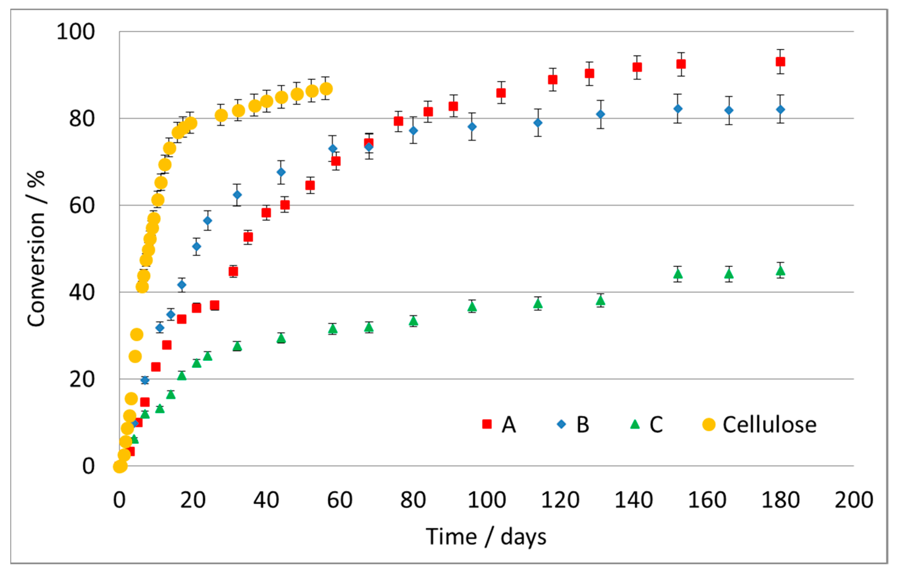
Figure 1 reports the conversion, as a percentage, as a function of time for the three tested samples of different materials and the cellulose used as reference.
The cellulose biodegradation data revealed very fast degradation in few days in the compost material used, assessing the validity of the test. It should be remembered that this test typically does not reach 100% conversion, since some carbon remains in the soil as part of the microorganism’s metabolism. The last linear part of the curve of the reference cellulose is considered as full degradation being accomplished.
These data were then processed by applying an integrated kinetic equation of the first order
where the time was expressed in days and k, the kinetic constant of the first order, expressed in days−1. Data obtained using reaction orders of 0 or 2 with respect to the substrate are reported in the Supporting Information file.
The maximum conversion achieved for the A formulate was ca. 93% after 180 days. The degradation rate strongly depends on the material itself and on particle size: here, the particles were very small, with a high surface area, which facilitates the attack and colonization by bacteria, and is not directly comparable with plastic foils, films, etc. Furthermore, formulates were used where the presence of pro-oxidants cannot be excluded to improve the degradability. Besides dependence on the material, it is important to note the different testing methods, burial materials and temperatures in the different data reported in the literature.
It should be noted that is not possible to directly estimate the conversion time of the polymer at 100% because the CO2 produced may not reach 100% compared with the theoretical, as stated above. In addition, it is noticed that a kinetic model of the first order does not admit the time estimate required for the conversion of 100% of the substrate, which would correspond to the computation of ln(0). We can then estimate the time required to achieve a conversion as close as desired to 100% (in our process: 90, 99, 99.9%).
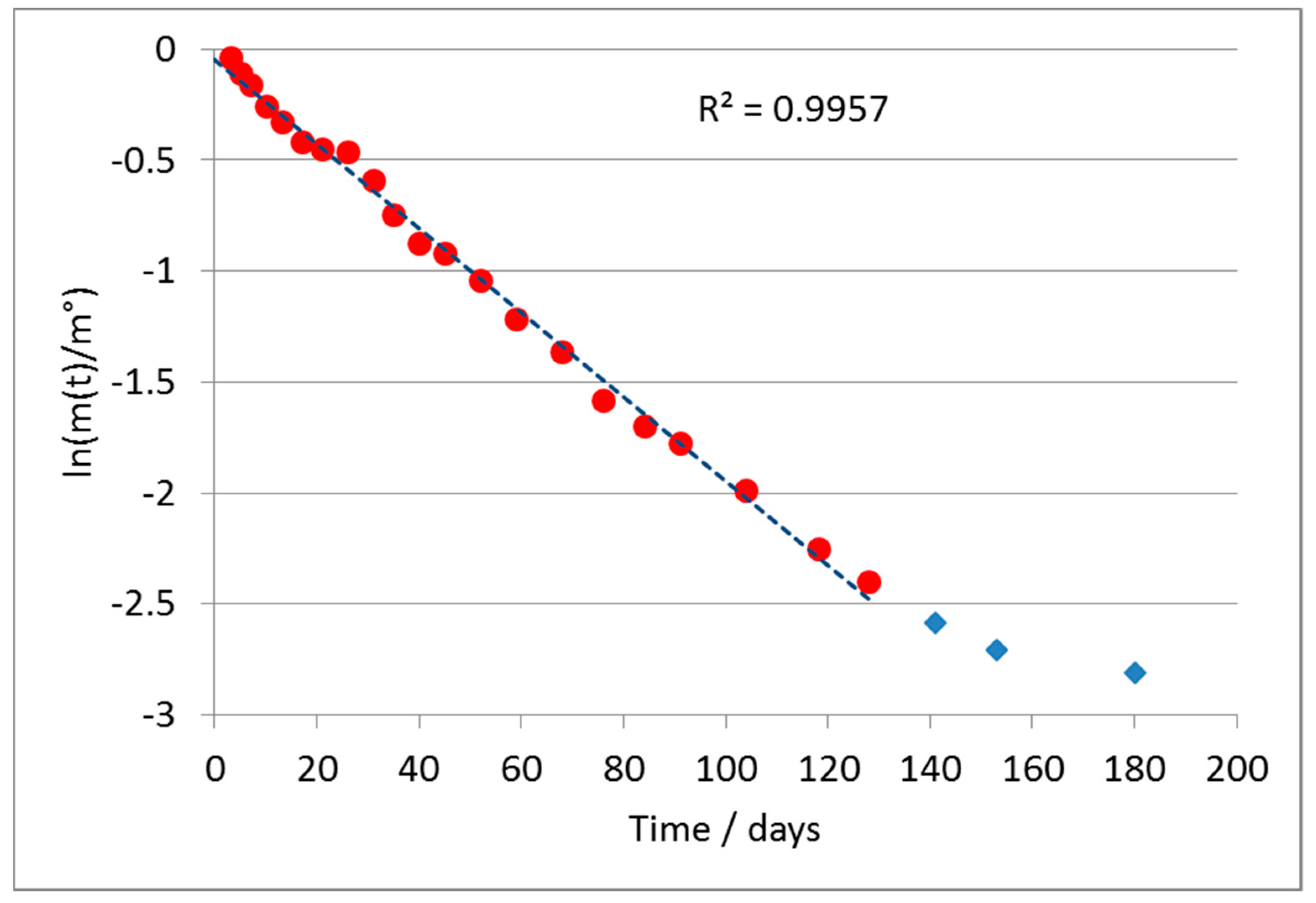
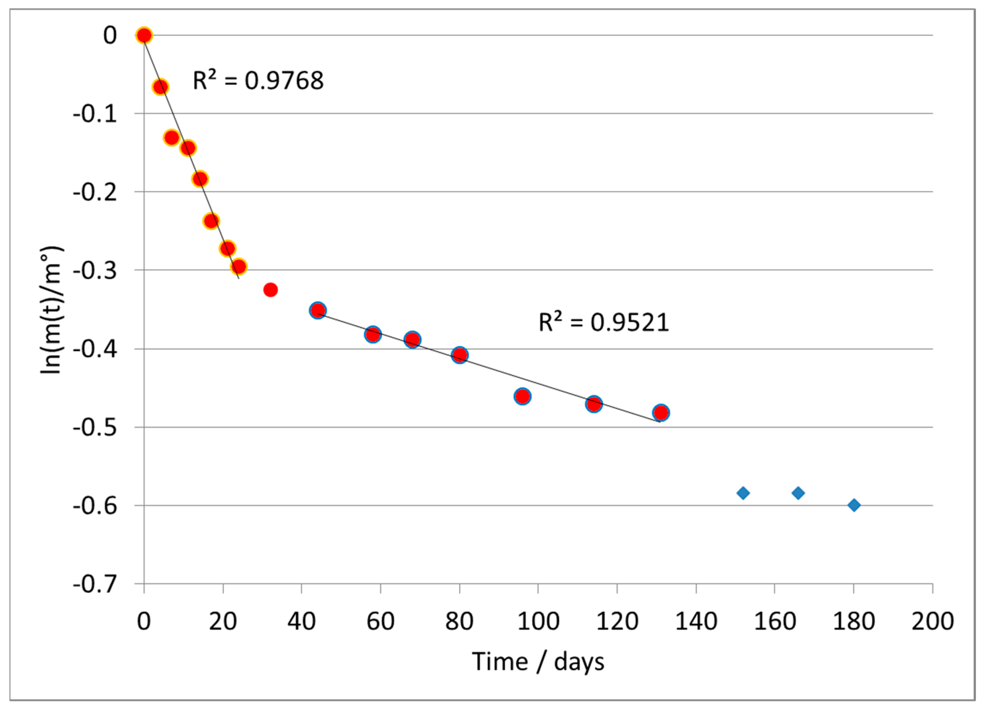
Representing the results according to Equation (4), a substantially linear trend was observed, confirming the validity of the assumption of a first-order kinetics, except for the last points of the test, in which the reaction was substantially complete. Figure 2 shows the results obtained from the linear regression of the curve according to the first-order model for the A formulate. The last three points, marked in blue, were considered outliers according to a statistical analysis of the deviance of their error (>300% in absolute value), from the mean value of the difference between the value calculated by the regression and the experimental one.
The absolute value of the slope of the line directly provides the value of the kinetic constant k, according to Equation (4). It was calculated as a value of k = 0.0204 ± 0.0010 days−1.
As verification, we calculated the half-life of the polymer, t1/2. For kinetics of first order, the calculation of the half-life is carried out with the following equation
t1/2 = ln(2)/k = 34 days
This result is perfectly in line with the experimental data, thus confirming the correct attribution of the reaction order. Then, the time required to biodegrade the polymer to 90%, 99%, 99.9% is estimated in Table 1.
The calculated data for the biodegradation of 90% of the material, 116 days, achieved further correspondence with the experimental data. It is noted, as said above, that it is impossible to estimate the time required to reach a 100% conversion for purely mathematic limits with this model, since it would be necessary calculate the ln(0). However, a concentration of residual polymer that is as low as desired can be entered in the formula, as long as it is different from 0.
The marked difference in the time taken for different conversions is due to the non-linear form of the model with respect to the concentration of the substrate. That is, when almost all the reagent is converted, the rate of the reaction slows down considerably, imposing longer times on the biodegradation of the residual material.
A model of enzyme biodegradation based on the Michaelis–Menten equation was also used to reprocess the data, applied in its linearized form according to a Lineweaver-Burk plot, where v is the degradation rate and vmax its maximum value, KM is the Michaelis constant and [S] is the substrate concentration.
This model led to a non-linear plot for substrate A, denoting that it is unsuitable to correctly fit the data. The elaboration led to a broad estimation of the degradation time with respect to the first-order model. Details are reported in the ESI, Figure S1, for the interested reader.
The application of integrated kinetic equations of orders zero and two with respect to the substrate was not satisfactory, as reported in the Electronic Supporting Information (ESI), Figures S2 and S3.
3.2. Material B
With an increase in the complexity of the polymer, we expect longer and possibly less complete biodegradation. The curve of biodegradation of formulate B (Figure 1) indicates an initially faster conversion, which then slows down with respect to sample A.
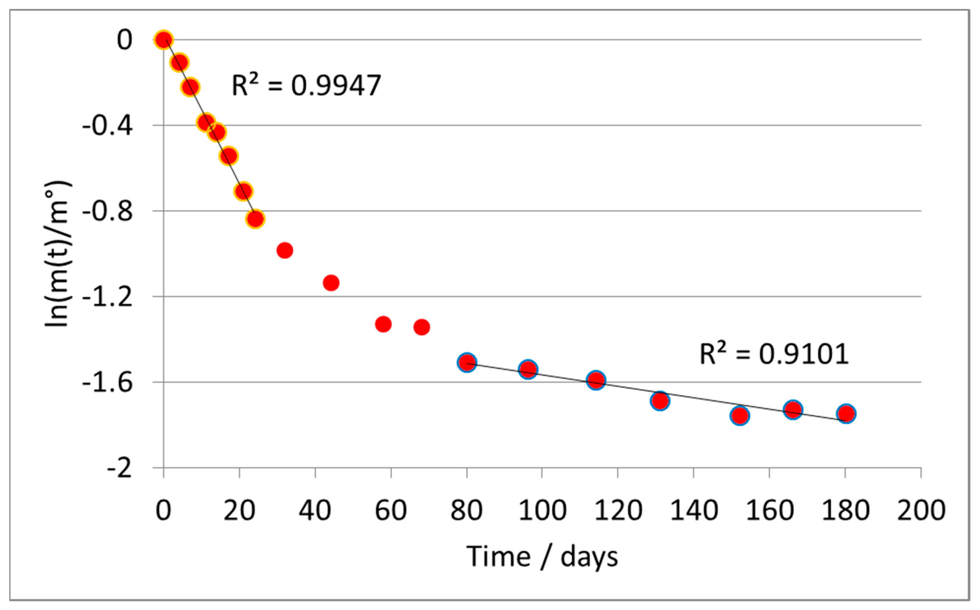
The same approach was used for data elaboration. In this case, the initial rate of biodegradation was very high, but after approximately 25 days, it underwent an abrupt slowdown, until it became negligible. The application of the same criteria of data-reprocessing throughout the whole experimental field has, however, produced a curve instead of a line, as shown in Figure 3.
This suggests the inadequacy of the first-order kinetic model in this case. Furthermore, the application of equations of order 0 or 2 did not produce significant improvements (see Supplementary Information).
Therefore, we adopted a different strategy. We assumed a reaction of order n
and we applied the method of Wilkinson for the determination of kinetic parameters [22].
dn/dt = k nn
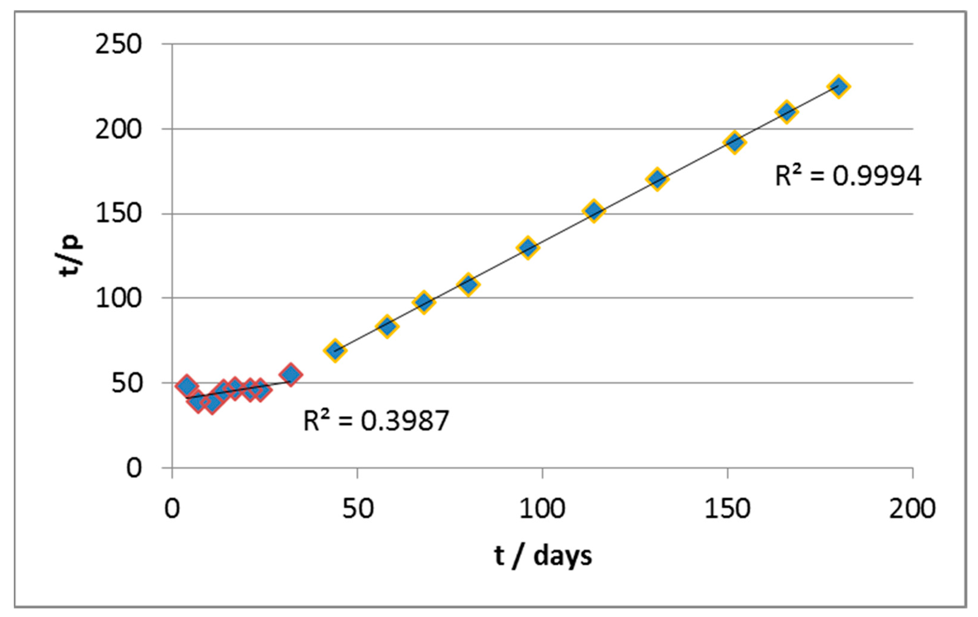
Approximately, it is possible to calculate a parameter p = 1-m/m° and to perform a linear regression of t/p vs. t, as follows
Therefore, the double of the slope of the line provides the estimated reaction order, while it is possible to estimate k from the intercept. According to this approach, we elaborated the kinetics of degradation of material B.
From the values of slope and intercepts, we estimated (Table 2) the values of n and k in the two curve sections (roughly active before and after 30 days (Figure 4).
In particular, it can be seen that in the early stages of the biodegradation, the estimated reaction order is <1 (as if there were product inhibition). The kinetics are also quite fast thanks to the relatively high value of k (as compared, for example, to material A) and the abundance of the substrate, which mitigates the slowing effect due to a fractional order of reaction. Notice that, in the first segment, the R2 value of the regression is severely low, partly for the scattered values, but also due to the very small slope of the curve, which is the main reason for the very low value of the correlation coefficient.
In the second section, on the other hand, the apparent order of reaction is higher and this, combined with the progressive consumption of substrate, leads to a significant slowing down of the reaction rate. In parallel, the fact that the curves of biodegradation practically reach a plateau is reflected in a kinetic constant which is orders of magnitude lower with respect to the previous section.
Using these kinetic data, we made two predictions, including the conversion in the experimental field to test the reliability of the model (Table 3):
From these data, it is evident that the first section (t < 30 days) is effectively described by the model. In the second section, the prevision is reasonable, although underestimated by 8–10%. The kinetic data of the second segment were used to estimate the time of biodegradation to 90%, 99% and 99.9% with the results reported in Table 1. By contrast, the first-order model underestimates the biodegradation time to achieve 20% conversion and poorly fits the prediction of 70% conversion.
We are interested in the prediction of the ultimate biodegradation, so the most interesting part of the curve is the one at higher times. The first part is also the most dependent on the possible presence of additives and pro-oxidants. The data reported in Table 3 show that the predicted time for 20% biodegradation is better calculated by the Wilkinson model, even if the almost horizontal fitting curve has a lower correlation coefficient.
Therefore, it is highly recommended to compare the kinetic models, not only for their fitting ability, but for their overall capacity to correctly represent the whole dataset.
Finally, we applied the Michaelis–Menten, zero-order and second-order models also to material B (see ESI), Figures S4–S6. The reprocessing of the data led to the same problems highlighted for material A.
3.3. Material C
The set of data for the formulate C (Figure 1) shows only a partial conversion of the polymer at the end of the test and a sharp downturn in reaction rate after the first 20–25 days. There is a rapid digestion of approximately 20% of the initial mass of the polymer and a subsequent slowdown. This could be due to a sequential mechanism of attack, according to which the chain is first broken and is partially eliminated in a more degradable portion, e.g., an aliphatic chain; subsequently, it proceeds with the biodegradation of the less degradable residual, for instance, an aromatic ring, which is considerably more resistant. This may explain the evolution of the curve, which slows down after 30 days, without reaching a net plateau.
Applying the first-order model (Figure 5) led again to a broken line, and in this case we separately treated the two branches of the curve.
In particular, we discuss the data of the second branch, since the first section does not clearly represent the rate-determining step of the reaction, as already discussed for previous types of material. The average value of the kinetic constant (second branch) was k = 0.00200 ± 0.00012 days−1.
The calculated halving time using k2 was 345 days, but there are no experimental data to check this value. However, this forecast seems to be reasonable, observing the available experimental data. In fact, the biodegradation of ca. 20–25% of the polymer occurs in ca. 155 days (excluding the first period of 25 days, in which the kinetic was much faster and converted ca. 20% of the substrate). It therefore seems likely that 345 days following the slowest kinetics can lead to 50% conversion.
Accordingly, we estimated the following conversion times for biodegradation of 90%, 99% and 99.9% of the substrate (Table 1).
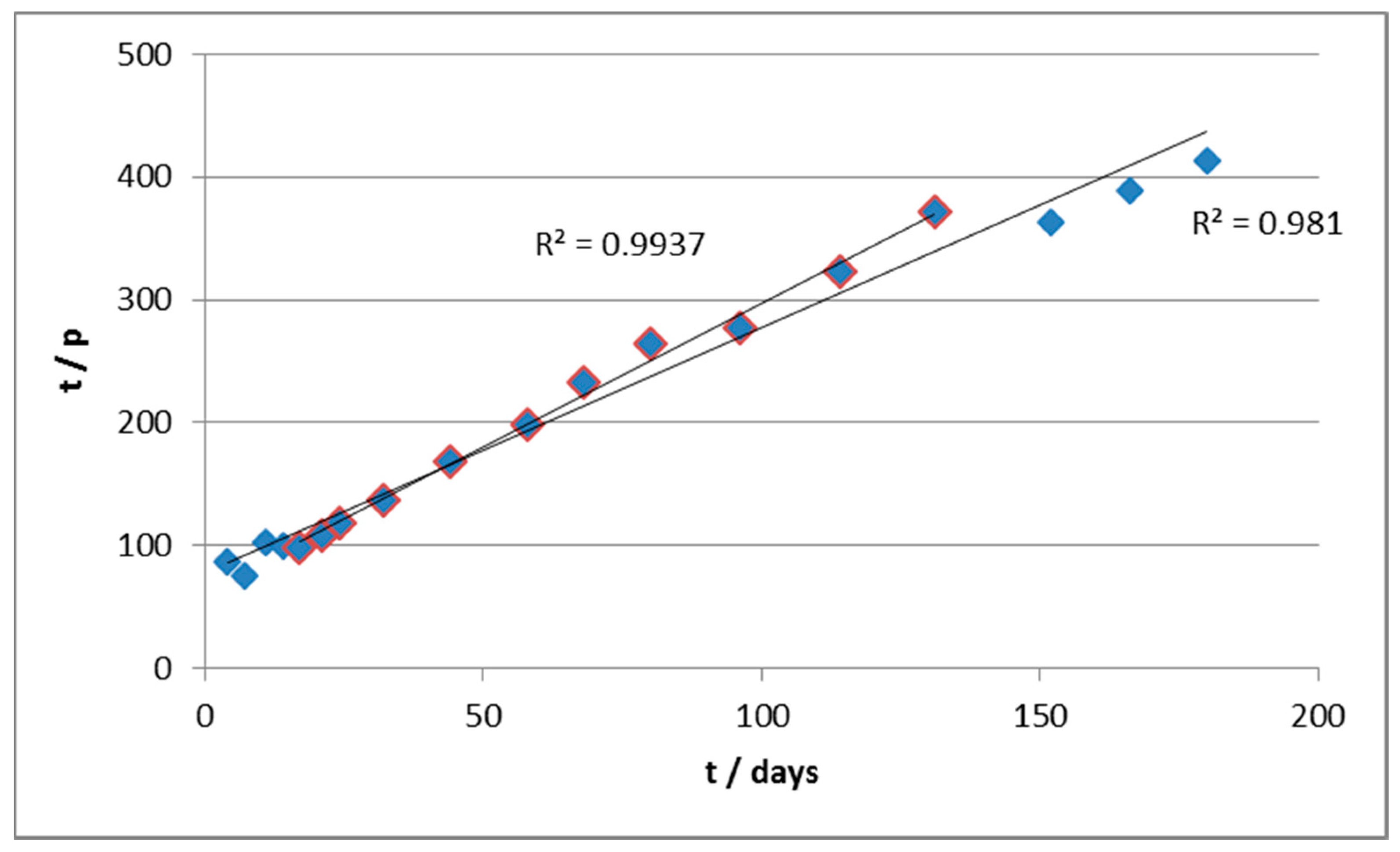
We also applied the Wilkinson model to this substrate (Figure 6). The reprocessing led to an apparent value of reaction order n = 4.2, with values of k in the order of 10−8 day−1 mg−3. Using these data to determine the time taken to reach 20% conversion returns an estimate of 25 days, broadly comparable with the experimental value. However, when one tries to provide the trend in the longer term, the deviations between calculated and experimental data become unacceptable. Even when excluding the last three points, which were again defined as outliers according to statistical analysis of the error distribution, the estimated parameters were n = 5.1 and k in the order of 10−10 day−1 mg−3, leading to overall unreliable predictions. The calculated time for biodegradation of 20% of the substrate was 20.1 days vs. 21 in the experimental, while for 30% biodegradation it was 44.7 days vs. 80 experimental.
This approach was, therefore, abandoned for material C, in spite of the quite good quality of data regression, also testified by the higher R2 value with respect to the first-order model, because it does not allow the weighting of the different branches of the curve, which likely rely on different mechanisms.
The Michaelis–Menten, zero-order and second-order models were also unsatisfactory when applied to this sample (see ESI), Figures S7–S9.
3.4. General Remarks
This work does not aim to provide evidence for or to discuss the biodegradability behavior of the tested materials, but rather to propose a kinetic approach to the elaboration of the degradability data (collected on whichever material) for a better comparison between different samples and tests.
Polyolefins represent the most widely used polymers, especially in the commercialization of single-use manufacts, such as food and beverage packaging. Pure polyethylene (i.e., not treated or combined with pro-oxidants) is extremely recalcitrant to degradation by abiotic or biotic factors, demonstrating limited mass loss after burial in humid soil for several years. Its resistance is due to concomitant factors. The hydrophobic chain prevents attack and colonization by microbials, which also cannot digest high-molecular-weight entities. Indeed, these molecules cannot enter microbial cells to be digested by intracellular enzymes and they are inaccessible to extracellular enzymes because of their excellent barrier properties. This is even more severe when increasing the crystallinity degree. As an example, UV-irradiation of polyethylene for 16 days before burial in soil produced less than 0.5 wt% carbon after 10 years, while in that without any pretreatment, less than 0.2 wt% CO2 was observed [23].
Thus, in order to circumvent this exceptional stability that brings environmental accumulation, different strategies have been formulated to improve the biodegradability of plastic-based objects prepared from conventional polymers, hence maintaining their functionality and processing advantages.
Possible pretreatments and the use of additives deeply modify the biodegradation of the material, in order to improve the abiotic steps of oxidation and to favour subsequent biotic action. For instance, a high-density PE film was chemically treated by immersion into KMnO4/HCl at for 8 h and 10% citric acid for 8 h at 45 °C. The HDPE degradation gradually increased from 9.4 to 20.8%, indicating synergism between biotic and abiotic factors [5]. Various transition-metal-based additives (traces of Mn, Fe, Co, Ti, e.g., as stearate or oleate) are also well known to improve the biodegradability thanks to an increase in the hydrofilicity and preliminary oxidation of the chain. A total of 70% degradation of a pre-oxidized high-molecular-weight polyethylene sample has been reported after 15 days of treatment with P. chrysosporium strain MTCC-787 [24]. Furthermore, the TDPA technology combines a transition metal carboxylate and an aliphatic poly (hydroxyl–carboxyl acid) [25]: samples of low-density PE films were tested with ca. 50–60% degradation after 18 months in soil. After 70 weeks, no fragments were collected from the soil [26]. Moreover, oxygenated compost columns at 50 °C to degrade PE films after fragmentation returned 60% mineralization after 400 days, whereas thermoformed PP films at 60 °C mineralized up to 60% in 700 days. The difference in degradation times was attributed to the different film thicknesses, since another important parameter is size [27].
It is clear that the search for a solution to the contingent issue of the scarce or nil biodegradability of packaging polymers has led to important results, but a plethora of pro-degradants are commercially available, as recently listed [14], and may be found in commercial formulates [5,28], often without clear indication: this further jeopardises the possibility of predicting the ultimate biodegradation time of such formulates.
In addition, the interest in the development of biodegradable plastics is rapidly raising, with a lot of composite materials that increase the degradability of the manufacts relying on more intrinsically degradable polymers where feasible (e.g., PLA), or on blending classic polyolefins with a biodegradable material (e.g., starch), often in concomitance with pro-oxidants. This wide variability of formulations is often unrecognizable in the disposed manufact, which reports only general indications on the base material (polyethylene, polypropylene, polystyrene, etc.) and on disposal prescriptions. Therefore, a more systematic approach towards degradation testing may help in comparing different formulations. We here propose a simplified kinetic modelling that may be useful to estimate the ultimate degradation time through modelling the aerobic biodegradation tests collected through a standardized method, whatever the tested material. This approach can be used to evaluate every batch of data of CO2 evolution vs. time.
Very wide formulations are currently commercialised. The presence of degradation enhancers may be one of the possible causes of the different degradation rates in the obtained curves. However, this does not affect the modelling methods, since promoters can have different effects. They can facilitate colonisation and attack by microorganisms or render the surface more prone to degradation (e.g., increasing hydrophilicity). In this case, one should see an overall increase in rate, but the mechanism remains practically the same and a pattern similar to material A is expected. In case the promoter instead implies limited durability (e.g., it degrades itself or gets lost in time, e.g., by leaching), one can expect an enhanced rate at the beginning of testing for the whole life of the material, so the overall curve manifests different slopes in time (as for materials B and C); in such a case, the expected ultimate degradation time should be considered from the slowest portion of the curve. The same variation in the curve is expected when the material is constituted of portions of the chain that can be more promptly attacked and portions that are harsher to degrade.
The particle size also deeply affects the degradation rate; examples of the testing of materials with different grain sizes can be found in the literature [11,13]. Fine comminution exposes more surface area and leads to easier formation of the biofilm, which is ultimately responsible for the biodegradation. Thus, the very small particles used in the present experiments cannot be compared with the rates observed for films, layers, etc. The wide variability of conditions and formulations contributes to the miscellaneous results landscape, making it really difficult to draw a general conclusion on the biodegradability of a material. Therefore, besides using standardized testing protocols, the use of well-defined data elaboration models would help obtain more uniform and comparable results.
The present data were elaborated using various kinetic models, highlighting their strengths and limitations. In every case, the elaboration was based on the best available kinetic models in the state of the art. The choice of the most appropriate kinetic models was made not only on the basis of the examination of the results, but also in light of some indications found in the literature. Specifically, A. Models et al. [29] underline that the biodegradation of polymeric materials in a homogeneous phase is properly describable by means of a Michaelis–Menten type kinetic model (enzyme kinetics), which is not entirely appropriate or properly extendable to the case of the aerobic final biodegradation of plastic materials under controlled composting conditions (see ESI). The application of a kinetic model of the first order represented a better representation of the results.
In support of this, another investigation [30] adopted a first-order kinetics approach. The authors also consider biodegradation that is possible via reactions in series, always of first order, when a period of initial induction is present in the formation of CO2. In other studies, a purely empirical strategy was adopted, by interpolating the data of CO2 formation as a function of time with mathematical models (not mechanistic) [31]. In such a case, it would be possible to calculate the time required for the formation of the theoretical amount of CO2 corresponding to complete biodegradation of the polymer. It should be recalled, however, that the models obtained by pure fitting of experimental data, not based on a verified mechanism of reaction, are usable for the forecasts within the adopted experimental field and not for extrapolation to a final degradation time longer than the experiment. Therefore, they are not the best option for long-term forecasting.
4. Conclusions
The ISO 14855 procedure represents a standard and reliable method to collect kinetic data for the biodegradation of different sets of polyolefin samples and of plastic materials in general. The main limit of this standard procedure is whether CO2 evolution is fully representative of biodegradation. Due to the fact that part of the carbon remains in the soil as part of the microorganisms, 100% conversion cannot physiologically be obtained. This effect can be managed by replicating the experiments and comparing the results with a blank (same conditions and environment but without the sample) and a reference degradable material.
Established kinetic models to interpret such data are currently scarce in the literature and a more quantitative assessment of the biodegradation pattern may be helpful regarding this point. Indeed, quantification of the rate of decomposition and its evolution over time better allows a comparison of materials. To this end, we proposed a comparison between rather simple kinetic models, to compute relevant kinetic parameters to interpret the biodegradation patterns of different materials. The data, expressed as CO2 formation as a function of time, can be easily elaborated through first-order kinetics, which were fully suitable to interpret the simplest cases, such as formulate A, which leads to a monotonous degradation curve. Zeroth- and second-order kinetic equations, however, were unsuitable for all the materials.
In some tests, a plateau conversion was reached, with apparent slowdown of the reaction. This can be due to either the exhaustion of compost activity, or to materials’ formulation (e.g., the presence of some unknown biodegradation-aiding additives, consumed during the reaction, or the mineralization of the weaker part of the polymer structure, leaving harsher fractions to be degraded slower).
The elaboration of the kinetic data for formulates B and C through a first-order kinetic model was not fully satisfactory, leading to a broken line. The kinetic constant derived from the regression allowed the calculation of reliable estimates of the time of half conversion of the substrate, and the time of final biodegradation of the compound, in every case. The Wilkinson model allowed for interpretation of the more complex curves in the case of materials B and C. The linear regression was particularly important in the second part of the curve, at a longer time, where data relevant to the final biodegradation can be derived. The Wilkinson model suggests the order of magnitude of the apparent reaction order and explains the slowdown of the process. The predictions by this model were more reliable for material B than C, which returned more satisfactory control data through the first-order model. Indeed, for material C, the prediction of the biodegradation time by the first-order model was better at adapting to the experimental data than the value predicted through the Wilkinson model. Finally, the Michaelis–Menten approach was adapted to the present case to estimate the maximum biodegradation rate and was marginally reliable only for the simpler substrates.
Overall, the easy-to-handle elaboration of data collected through a standard test proposed here can help to assess quantitative parameters to estimate the biodegradability of different substrates and to quantitatively compare the materials. It is highly recommended to rely on the whole analysis of the quality of fitting and of predictions, instead of considering strictly statistical parameters. For instance, models characterized by lower correlation coefficients were better able to represent the biodegradability than apparently better-fitting regressions.
As a general procedure, it is suggested to preliminarily interpret the degradation kinetic data through a simple first-order model. If correctly linearized (except after reaching a plateau or during an induction time), the kinetic parameters allow to predict the expected biodegradation time for the conversion of different amounts of material, until ultimate degradation. Instead, if the data give rise to a monotonous curve plot, the Wilkinson model can be used to assess the apparent order of reaction and the kinetic constant. A third option may arise when different degradation mechanisms are active, for instance when a portion of the polymer degrades faster, leaving a harsher residue to decompose. In such a case, the first faster decay rate can be discarded, and the later part of the curve interpreted to assess the ultimate degradation time, as in the example of material C.
Supplementary Materials
The following are available online at https://0-www-mdpi-com.brum.beds.ac.uk/2673-4117/2/1/5/s1, Decription of Michelis Menten, Zeroth and second order kinetic models, Figure S1: Michelis Menten elaboration according to a Lineweaver Burk plot of the biodegradation data of material A. Red void symbols represent a zoom of the linearization used, Figure S2: Zero order kinetic equation for the biodegradation data of material A, Figure S3: Second order kinetic equation for the biodegradation data of material A, Figure S4: Michelis Menten elaboration according to a Lineweaver Burk plot of the biodegradation data of material B. Red void symbols represent a zoom of the linearization used, Figure S5: Zero order kinetic equation for the biodegradation data of material B, Figure S6: Second order kinetic equation for the biodegradation data of material B, Figure S7: Michelis Menten elaboration according to a Lineweaver Burk plot of the biodegradation data of material C. Red void symbols represent a zoom of the linearization used, Figure S8: Zero order kinetic equation for the biodegradation data of material C, Figure S9: Second order kinetic equation for the biodegradation data of material C.
Author Contributions
Conceptualization, I.R.; methodology, F.C.; data curation, F.C.; writing—original draft preparation, G.R.; writing—review and editing, I.R.; supervision, G.R.; funding acquisition, I.R. All authors have read and agreed to the published version of the manuscript.
Funding
This research received no external funding.
Institutional Review Board Statement
Not applicable.
Informed Consent Statement
Not applicable.
Data Availability Statement
The data presented in this study are available in this paper and its Supplementary information file.
Conflicts of Interest
The authors declare no conflict of interest.
References
- Sam, S.T.; Nuradibah, M.; Ismail, A.H.; Noriman, N.Z.; Ragunathan, S. Recent advances in polyolefins/natural Polymer blends used for packaging application. Polym. Plast. Technol. Eng. 2014, 53, 631–644. [Google Scholar] [CrossRef]
- Galgani, L.; Loiselle, S. Plastic Accumulation in the Sea Surface Microlayer: An Experiment-Based Perspective for Future Studies. Geosciences 2019, 9, 66. [Google Scholar] [CrossRef] [Green Version]
- Ubeda, B.; Gálvez, J.Á.; Irigoien, X.; Duarte, C.M. Plastic accumulation in the Med sea water. PLoS ONE 2015, 10, e0121762. [Google Scholar]
- Barnes, D.K.A.; Galgani, F.; Thompson, R.C.; Barlaz, M. Accumulation and fragmentation of plastic debris in global environments. Philos. Trans. R. Soc. B Biol. Sci. 2009, 364, 1985–1998. [Google Scholar] [CrossRef] [Green Version]
- Ghatge, S.; Yang, Y.; Ahn, J.H.; Hur, H.G. Biodegradation of polyethylene: A brief review. Appl. Biol. Chem. 2020, 63, 1–14. [Google Scholar] [CrossRef]
- Restrepo-Flórez, J.M.; Bassi, A.; Thompson, M.R. Microbial degradation and deterioration of polyethylene—A review. Int. Biodeterior. Biodegrad. 2014, 88, 83–90. [Google Scholar] [CrossRef]
- Barton-Pudlik, J.; Czaja, K.; Grzymek, M.; Lipok, J. Evaluation of wood-polyethylene composites biodegradability caused by filamentous fungi. Int. Biodeterior. Biodegrad. 2017, 118, 10–18. [Google Scholar] [CrossRef]
- Fontanella, S.; Bonhomme, S.; Brusson, J.-M.; Pitteri, S.; Samuel, G.; Pichon, G.; Lacoste, J.; Fromageot, D.; Lemaire, J.; Delort, A.-M. Comparison of biodegradability of various polypropylene films containing pro-oxidant additives based on Mn, Mn/Fe or Co. Polym. Degrad. Stab. 2013, 98, 875–884. [Google Scholar] [CrossRef]
- Fontanella, S.; Bonhomme, S.; Koutny, M.; Husarova, L.; Brusson, J.-M.; Courdavault, J.-P.; Pitteri, S.; Samuel, G.; Pichon, G.; Lemaire, J.; et al. Comparison of the biodegradability of various polyethylene films containing pro-oxidant additives. Polym. Degrad. Stab. 2010, 95, 1011–1021. [Google Scholar] [CrossRef]
- Koutny, M.; Sancelme, M.; Dabin, C.; Pichon, N.; Delort, A.-M.; Lemaire, J. Acquired biodegradability of polyethylenes containing pro-oxidant additives. Polym. Degrad. Stab. 2006, 91, 1495–1503. [Google Scholar] [CrossRef] [Green Version]
- Funabashi, M.; Ninomiya, F.; Kunioka, M. Biodegradability evaluation of polymers by ISO 14855-2. Int. J. Mol. Sci. 2009, 10, 3635–3654. [Google Scholar] [CrossRef] [PubMed] [Green Version]
- Castro-Aguirre, E.; Auras, R.; Selke, S.; Rubino, M.; Marsh, T. Insights on the aerobic biodegradation of polymers by analysis of evolved carbon dioxide in simulated composting conditions. Polym. Degrad. Stab. 2017, 137, 251–271. [Google Scholar] [CrossRef] [Green Version]
- Arutchelvi, J.; Sudhakar, M.; Arkatkar, A.; Doble, M.; Bhaduri, S.; Uppara, P.V. Biodegradation of polyethylene and polypropylene. Indian J. Biotechnol. 2008, 7, 9–22. [Google Scholar]
- Ammala, A.; Bateman, S.; Dean, K.; Petinakis, E.; Sangwan, P.; Wong, S.; Yuan, Q.; Yu, L.; Patrick, C.; Leong, K.H. An Overview of Degradable and Biodegradable Polyolefins; Elsevier Ltd.: Amsterdam, The Netherlands, 2011; Volume 36. [Google Scholar]
- Dřímal, P.; Hoffmann, J.; Družbík, M. Evaluating the aerobic biodegradability of plastics in soil environments through GC and IR analysis of gaseous phase. Polym. Test. 2007, 26, 729–741. [Google Scholar] [CrossRef]
- Nguyen, D.M.; Do, T.V.V.; Grillet, A.-C.; Ha Thuc, H.; Ha Thuc, C.N. Biodegradability of polymer film based on low density polyethylene and cassava starch. Int. Biodeterior. Biodegrad. 2016, 115, 257–265. [Google Scholar] [CrossRef]
- Ali, H.E.; Abdel Ghaffar, A.M. Preparation and Effect of Gamma Radiation on The Properties and Biodegradability of Poly(Styrene/Starch) Blends. Radiat. Phys. Chem. 2017, 130, 411–420. [Google Scholar] [CrossRef]
- Kawai, F.; Watanabe, M.; Shibata, M.; Yokoyama, S.; Sudate, Y. Experimental analysis and numerical simulation for biodegradability of polyethylene. Polym. Degrad. Stab. 2002, 76, 129–135. [Google Scholar] [CrossRef]
- Ramis, X.; Cadenato, A.; Salla, J.M.; Morancho, J.M.; Vallés, A.; Contat, L.; Ribes, A. Thermal degradation of polypropylene/starch-based materials with enhanced biodegradability. Polym. Degrad. Stab. 2004, 86, 483–491. [Google Scholar] [CrossRef]
- Kunioka, M.; Ninomiya, F.; Funabashi, M. Novel evaluation method of biodegradabilities for oil-based polycaprolactone by naturally occurring radiocarbon-14 concentration using accelerator mass spectrometry based on ISO 14855-2 in controlled compost. Polym. Degrad. Stab. 2007, 92, 1279–1288. [Google Scholar] [CrossRef]
- Massardier-Nageotte, V.; Pestre, C.; Cruard-Pradet, T.; Bayard, R. Aerobic and anaerobic biodegradability of polymer films and physico-chemical characterization. Polym. Degrad. Stab. 2006, 91, 620–627. [Google Scholar] [CrossRef]
- Connors, K.A. Chemical Kinetics; VCH Publishers, Inc.: Hoboken, NJ, USA, 1990. [Google Scholar]
- Albertsson, A.; Karlsson, S. The influence of biotic and abiotic environments on the degradation of polyethylene. Prog. Polym. Sci. 1990, 15, 177–192. [Google Scholar] [CrossRef]
- Mukherjee, S.; Kundu, P. Alkaline fungal degradation of oxidized polyethylene in black liquor: Studies on the effect of lignin peroxidases and manganese peroxidases. J. Appl. Polym. Sci. 2014, 131, 40738. [Google Scholar] [CrossRef]
- Garcia, R.; Gho, J. Degradable/Compostable Concentrates, Process for Making Degradable/Compostable Packaging Materials and the Products Thereof. U.S. Patent 5,854,304A, 29 December 1998. [Google Scholar]
- Chiellini, E.; Corti, A.; Swift, G. Biodegradation of thermally-oxidized, fragmented low-density polyethylenes. Polym. Degrad. Stab. 2003, 81, 341–351. [Google Scholar] [CrossRef]
- Available online: https://www.reverteplastics.com/ (accessed on 1 February 2021).
- Scott, G.; Wiles, D.M. Programmed-life plastics from polyolefins: A new look at sustainability. Biomacromolecules 2001, 2, 615–622. [Google Scholar] [CrossRef] [PubMed]
- Modelli, A.; Calcagno, B.; Scandola, M. Kinetics of Aerobic Polymer Degradation in Soil by Means of the ASTM D 5988-96 Standard Method. J. Envrion. Polym. Degrad. 1999, 7, 109. [Google Scholar] [CrossRef]
- Leejarkpai, T.; Suwanmanee, U.S.; Rudeekit, Y.; Mungcharoen, T. Biodegradable kinetics of plastics under controlled composting conditions. Waste Manag. 2011, 31, 1153. [Google Scholar] [CrossRef]
- Mohee, R.; Unmar, G.D.; Mudhoo, A.; Khadoo, P. Biodegradability of biodegradable/degradable plastic materials under aerobic and anaerobic conditions. Waste Manag. 2008, 28, 1624–1629. [Google Scholar] [CrossRef]
Figure 1.
Conversion (%) of the three commercial samples and reference cellulose as a function of time.
Figure 1.
Conversion (%) of the three commercial samples and reference cellulose as a function of time.

Figure 2.
Linear regression of the conversion data for the A formulate according to the first-order model (Equation (4)). Blue diamonds were not included in the regression pertaining to the plateau region.
Figure 2.
Linear regression of the conversion data for the A formulate according to the first-order model (Equation (4)). Blue diamonds were not included in the regression pertaining to the plateau region.

Figure 3.
Elaboration of the data of three samples of formulate B according to the first-order model.
Figure 3.
Elaboration of the data of three samples of formulate B according to the first-order model.

Figure 4.
Elaboration of the kinetic data of formulate B according to the Wilkinson model.

Figure 5.
Linear regression of the curve of conversion of material C according to the first-order model. Blue diamonds were considered as outliers and not included in the regression.
Figure 5.
Linear regression of the curve of conversion of material C according to the first-order model. Blue diamonds were considered as outliers and not included in the regression.

Figure 6.
Regression of the curve of conversion of material C according to the Wilkinson model. Last three points included or not included in the regression.
Figure 6.
Regression of the curve of conversion of material C according to the Wilkinson model. Last three points included or not included in the regression.


Table 1.
Calculation of the final biodegradation time corresponding to the conversion of 90, 99 and 99.9% conversion for the different materials.
Table 1.
Calculation of the final biodegradation time corresponding to the conversion of 90, 99 and 99.9% conversion for the different materials.
| A a | B b | C a | |||
|---|---|---|---|---|---|
| Conv. | Estimated Time (Days) | Estimated Time (Days) | Estimated Time (Years) | Estimated Time (Days) | Estimated Time (Years) |
| 90% | 116 | 227 | 0.62 | 1200 | 3.3 |
| 99% | 230 | 5501 | 15.1 | 2380 | 6.5 |
| 99.90% | 340 | 100,300 | 275 | 3530 | 9.7 |
a Estimated from first order kinetics. b Estimated from the Wilkinson model.
Table 2.
Kinetic parameters for the Wilkinson Model used to interpret the biodegradation of formulate B.
Table 2.
Kinetic parameters for the Wilkinson Model used to interpret the biodegradation of formulate B.
| n | k (day−1 mg−0.3) | |
|---|---|---|
| <30 days | 0.71 | 0.14 ± 0.05 (k1) |
| >30 days | 2.5 | (5.37 ± 0.15) 10−5 (k2) |
Table 3.
Calculation of the biodegradation time (days) corresponding to the conversion of 20 and 70% of the material in comparison with the experimental datum.
Table 3.
Calculation of the biodegradation time (days) corresponding to the conversion of 20 and 70% of the material in comparison with the experimental datum.
| 1st Order Model | Wilkinson Model | ||||
|---|---|---|---|---|---|
| Conversion | Estimated Time Using k1 | Estimated Time Using k2 | Estimated Time Using k1 | Estimated Time Using k2 | Experimental |
| 20% | 6 | - | 8.3 | - | 9 |
| 70% | - | 83 | - | 51 | 58 |
| 99% | - | 1706 | - | 5501 | - |
Publisher’s Note: MDPI stays neutral with regard to jurisdictional claims in published maps and institutional affiliations. |
© 2021 by the authors. Licensee MDPI, Basel, Switzerland. This article is an open access article distributed under the terms and conditions of the Creative Commons Attribution (CC BY) license (http://creativecommons.org/licenses/by/4.0/).
Share and Cite
MDPI and ACS Style
Rossetti, I.; Conte, F.; Ramis, G. Kinetic Modelling of Biodegradability Data of Commercial Polymers Obtained under Aerobic Composting Conditions. Eng 2021, 2, 54-68. https://0-doi-org.brum.beds.ac.uk/10.3390/eng2010005
AMA Style
Rossetti I, Conte F, Ramis G. Kinetic Modelling of Biodegradability Data of Commercial Polymers Obtained under Aerobic Composting Conditions. Eng. 2021; 2(1):54-68. https://0-doi-org.brum.beds.ac.uk/10.3390/eng2010005
Chicago/Turabian StyleRossetti, Ilenia, Francesco Conte, and Gianguido Ramis. 2021. "Kinetic Modelling of Biodegradability Data of Commercial Polymers Obtained under Aerobic Composting Conditions" Eng 2, no. 1: 54-68. https://0-doi-org.brum.beds.ac.uk/10.3390/eng2010005