
Evaluation and Prediction of the Impacts of Land Cover Changes on Hydrological Processes in Data Constrained Southern Slopes of Kilimanjaro, Tanzania

 , and
, and
Abstract
:1. Introduction
2. Materials and Methods
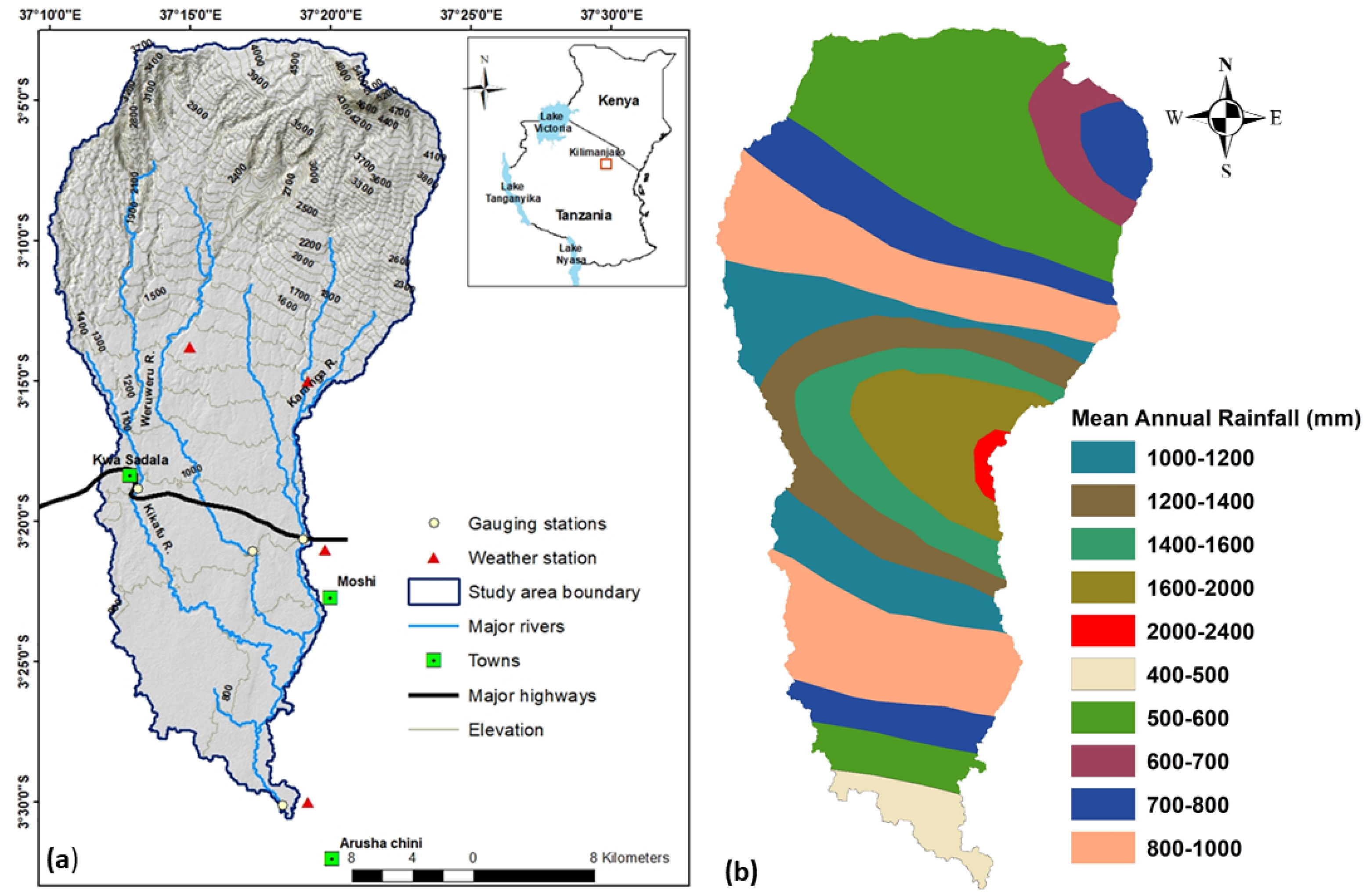
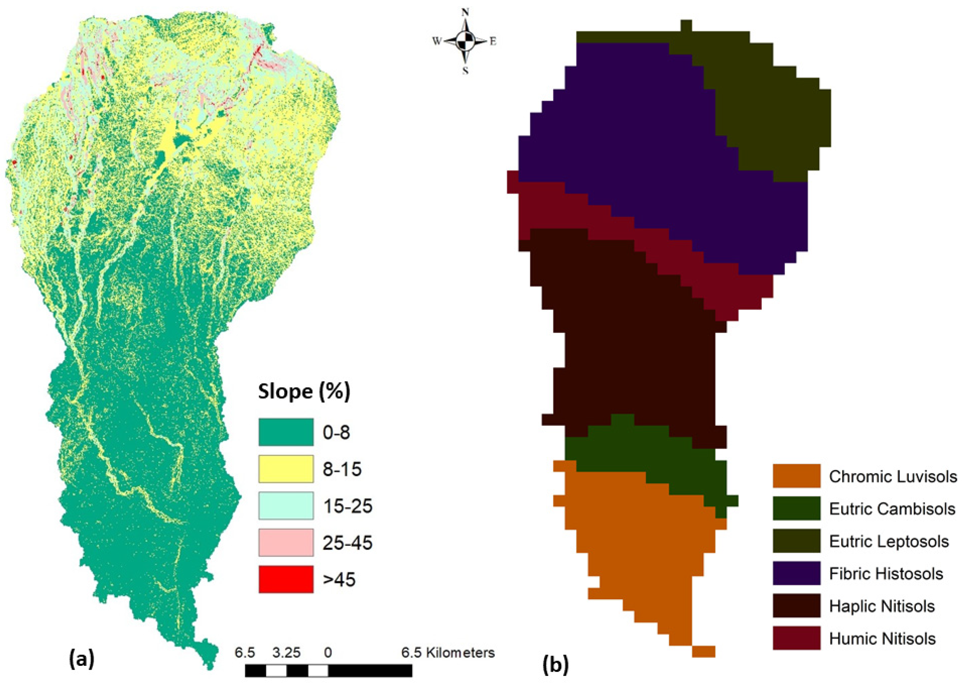
2.1. The Study Area
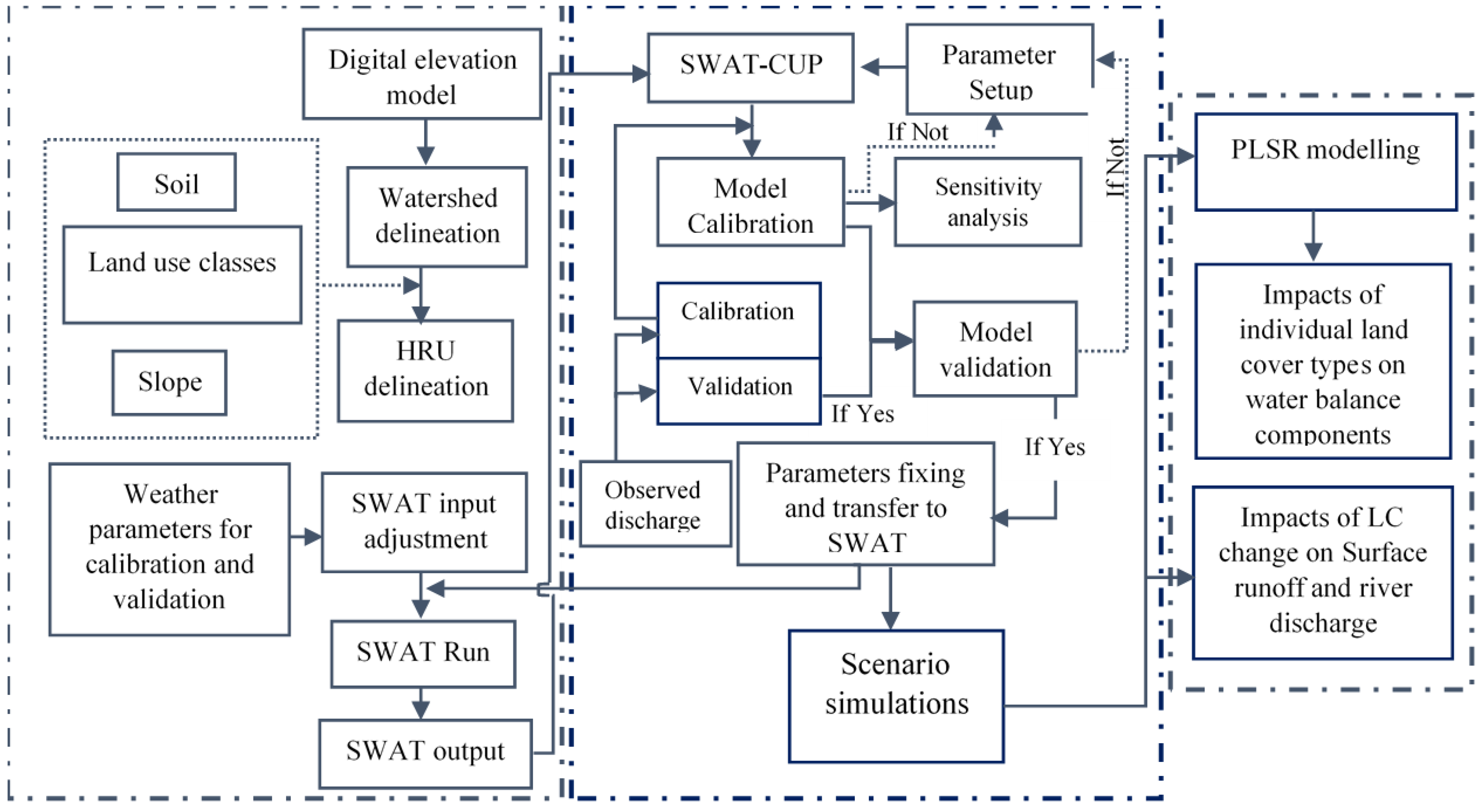
2.2. The General Approach of the Study
2.3. Soil and Water Assessment Tool (SWAT)
2.4. ArcSWAT Model Input Data
2.5. Model Set-Up and Parameterization
2.6. Automatic Calibration and Validation of the SWAT Model
2.7. Partial Least Squares Regression Analysis
2.8. Simulation of Impacts of LU Change Scenarios on Hydrological Processes
3. Results
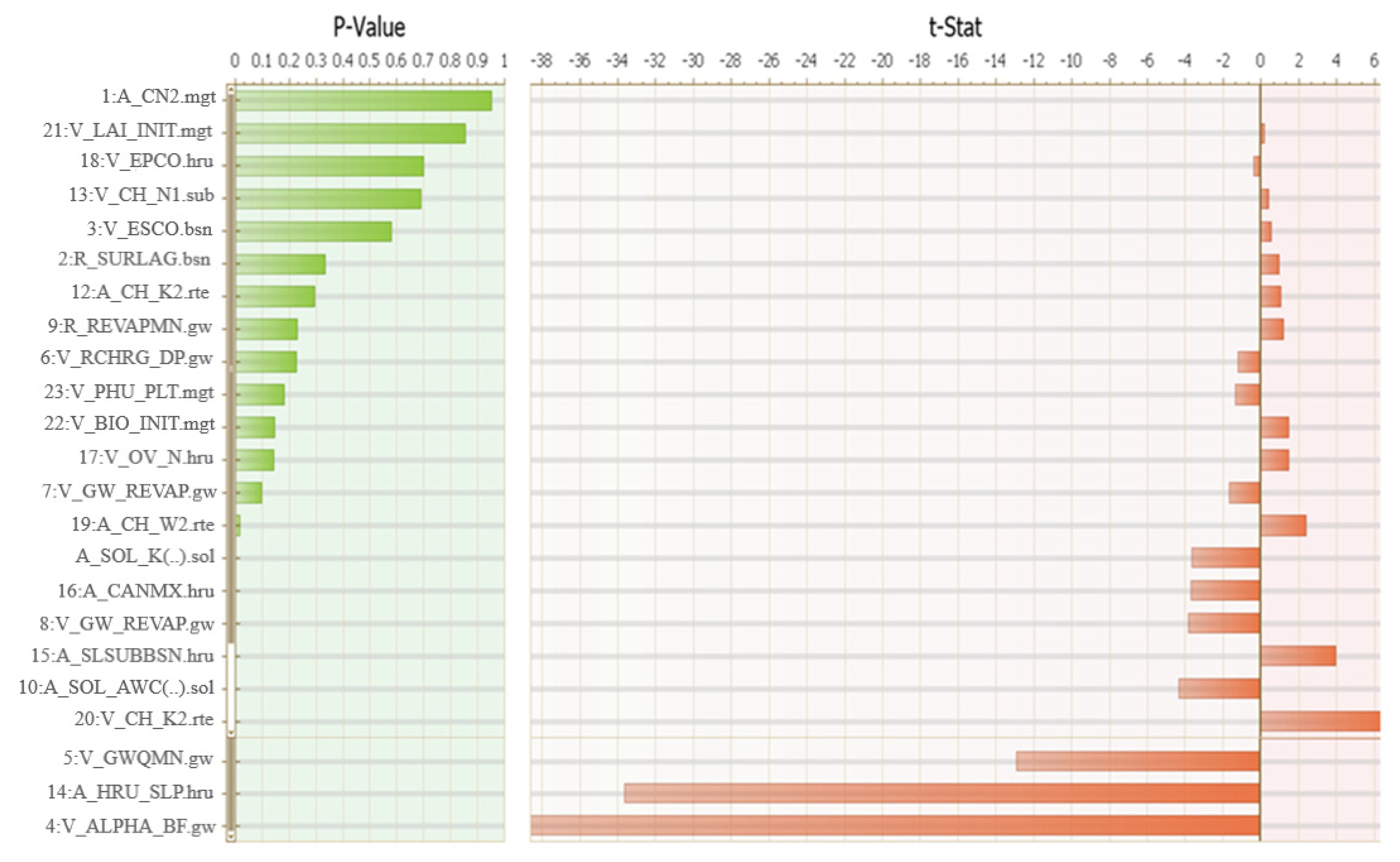
3.1. Sensitivity Analysis
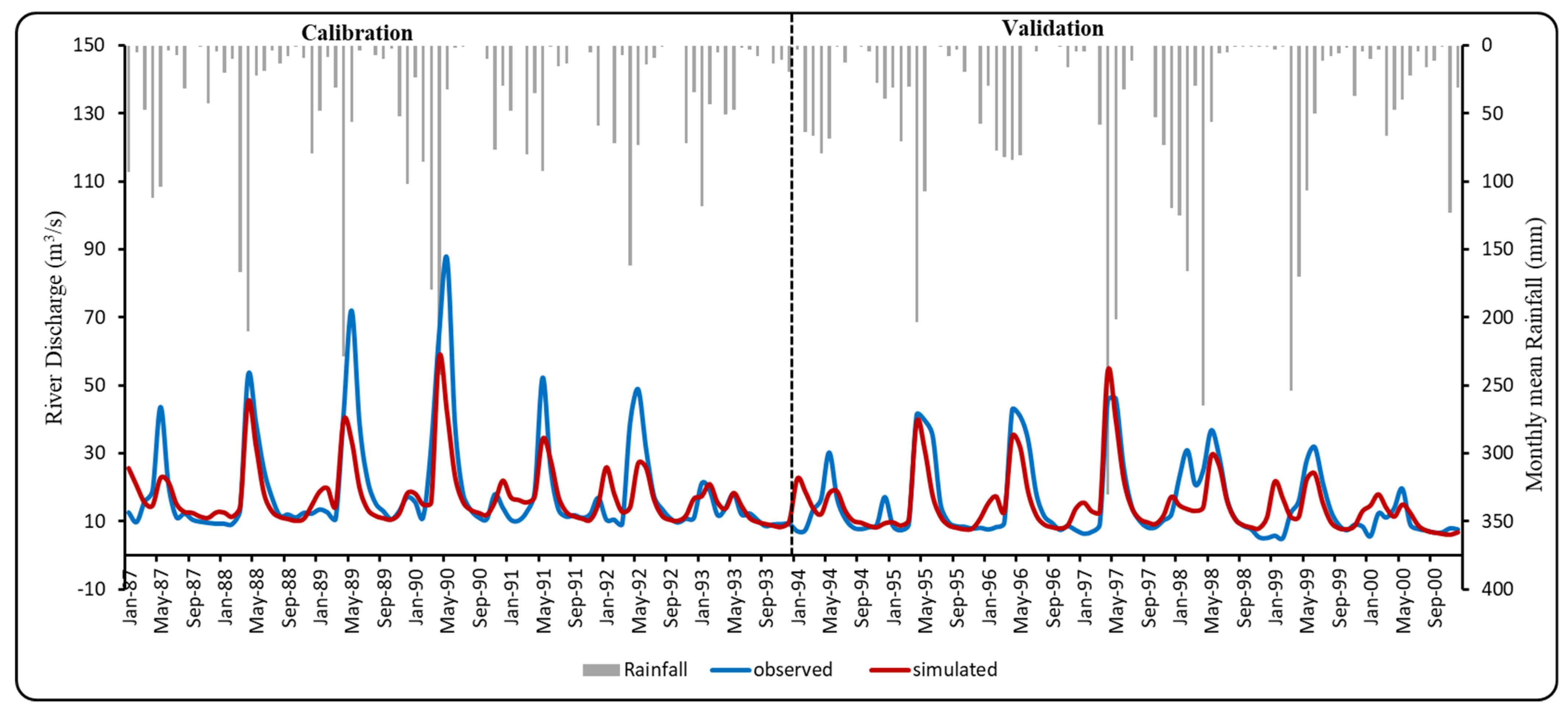
3.2. Model Parameters, Calibration and Validation
3.3. The Impact of Land Cover Changes on the Hydrology of the KWK Watershed
3.4. The PLSR Model Explained Variations of Individual Land Cover Changes on Water Balance
3.5. Hydrological Impacts of Individual Land Cover Changes on the Selected Water Balance Components
4. Discussion
4.1. Sensitivity Analysis
4.2. Model Parameters, Calibration and Validation
4.3. The Impact of Land Cover Changes on the Hydrology of the KWK Watershed
4.4. The PLSR Model Explained Variations of Individual Land Cover Changes on Water Balance
4.5. Hydrological Impacts of Individual Land Cover Changes on the Selected Water Balance Components
5. Conclusions
Limitations of the Study
Author Contributions
Funding
Data Availability Statement
Acknowledgments
Conflicts of Interest
References
- Zhou, Y.; Xu, Y.J.; Xiao, W.; Wang, J.; Huang, Y.; Yang, H. Climate Change Impacts on Flow and Suspended Sediment Yield in Headwaters of High-Latitude Regions—A Case Study in China’s Far Northeast. Water 2017, 9, 966. [Google Scholar] [CrossRef] [Green Version]
- Briones, R.; Ella, V.; Bantayan, N. Hydrologic impact evaluation of land use and land cover change in Palico Watershed, Batangas, Philippines Using the SWAT model. J. Environ. Sci. Manag. 2016, 19, 96–107. [Google Scholar]
- Neupane, R.P.; Kumar, S. Estimating the effects of potential climate and land use changes on hydrologic processes of a large agriculture dominated watershed. J. Hydrol. 2015, 529, 418–429. [Google Scholar] [CrossRef]
- Karimi, H.; Jafarnezhad, J.; Khaledi, J.; Ahmadi, P. Monitoring and prediction of land use/land cover changes using CA-Markov model: A case study of Ravansar County in Iran. Arab. J. Geosci. 2018, 11, 592. [Google Scholar] [CrossRef]
- Gashaw, T.; Tulu, T.; Argaw, M.; Worqlul, A.W. Modeling the hydrological impacts of land use/land cover changes in the Andassa watershed, Blue Nile Basin, Ethiopia. Sci. Total Environ. 2018, 619–620, 1394–1408. [Google Scholar] [CrossRef] [PubMed]
- Olson, J.M.; Alagarswamy, G.; Andresen, J.A.; Campbell, D.J.; Davis, A.Y.; Ge, J.; Huebner, M.; Lofgren, B.M.; Lusch, D.P.; Moore, N.J.; et al. Integrating diverse methods to understand climate–land interactions in East Africa. Geoforum 2008, 39, 898–911. [Google Scholar] [CrossRef]
- Baldus, R.D.; Hahn, R.; Mpanduji, D.G.; Siege, L. The selous-niassa wildlife corridor. Tanzania Wildlife Discussion Series 2003. Available online: http://www.suaire.sua.ac.tz/handle/123456789/2072 (accessed on 17 May 2021).
- Kitalika, A.J.; Machunda, R.L.; Komakech, H.C.; Njau, K.N. Land-Use and Land Cover Changes on the Slopes of Mount Meru-Tanzania. Curr. World Environ. 2018, 13, 331–352. [Google Scholar] [CrossRef] [Green Version]
- Kashaigili, J.; Majaliwa, A. Implications of land use and land cover changes on hydrological regimes of the Malagarasi River, Tanzania. J. Agric. Sci. Appl. 2013, 2, 45–50. [Google Scholar] [CrossRef]
- Marhaento, H.; Booij, M.J.; Hoekstra, A. Hydrological response to future land-use change and climate change in a tropical catchment. Hydrol. Sci. J. 2018, 63, 1368–1385. [Google Scholar] [CrossRef] [Green Version]
- Yadav, S.; Babel, M.S.; Shrestha, S.; Deb, P. Land use impact on the water quality of large tropical river: Mun River Basin, Thailand. Environ. Monit. Assess. 2019, 191, 614. [Google Scholar] [CrossRef]
- Yin, Z.; Feng, Q.; Yang, L.; Wen, X.; Si, J.; Zou, S. Long Term Quantification of Climate and Land Cover Change Impacts on Streamflow in an Alpine River Catchment, Northwestern China. Sustainability 2017, 9, 1278. [Google Scholar] [CrossRef] [Green Version]
- Zhang, L.; Karthikeyan, R.; Bai, Z.; Srinivasan, R. Analysis of streamflow responses to climate variability and land use change in the Loess Plateau region of China. Catena 2017, 154, 1–11. [Google Scholar] [CrossRef]
- Foley, J.A.; DeFries, R.; Asner, G.P.; Barford, C.; Bonan, G.; Carpenter, S.R.; Chapin, F.S.; Coe, M.T.; Daily, G.C.; Gibbs, H.K.; et al. Global Consequences of Land Use. Science 2005, 309, 570–574. [Google Scholar] [CrossRef] [PubMed] [Green Version]
- Memarian, H.; Balasundram, S.K.; Abbaspour, K.C.; Talib, J.B.; Sung, C.T.B.; Sood, A.M. SWAT-based hydrological modelling of tropical land-use scenarios. Hydrol. Sci. J. 2014, 59, 1808–1829. [Google Scholar] [CrossRef]
- Fohrer, N.; Haverkamp, S.; Eckhardt, K.; Frede, H.-G. Hydrologic Response to land use changes on the catchment scale. Phys. Chem. Earth Part B Hydrol. Oceans Atmosphere 2001, 26, 577–582. [Google Scholar] [CrossRef]
- Abe, C.A.; Lobo, F.D.L.; Dibike, Y.B.; Costa, M.P.D.F.; Dos Santos, V.; Novo, E.M.L.M. Modelling the Effects of Historical and Future Land Cover Changes on the Hydrology of an Amazonian Basin. Water 2018, 10, 932. [Google Scholar] [CrossRef] [Green Version]
- Dos Santos, V.; Laurent, F.; Abe, C.; Messner, F. Hydrologic Response to Land Use Change in a Large Basin in Eastern Amazon. Water 2018, 10, 429. [Google Scholar] [CrossRef] [Green Version]
- Fu, B.-J.; Wang, Y.-F.; Lu, Y.-H.; He, C.-S.; Chen, L.-D.; Song, C.-J. The effects of land-use combinations on soil erosion: A case study in the Loess Plateau of China. Prog. Phys. Geogr. Earth Environ. 2009, 33, 793–804. [Google Scholar] [CrossRef]
- Defersha, M.B.; Melesse, A.M. Field-scale investigation of the effect of land use on sediment yield and runoff using runoff plot data and models in the Mara River basin, Kenya. Catena 2012, 89, 54–64. [Google Scholar] [CrossRef]
- Shawul, A.A.; Chakma, S.; Melesse, A.M. The response of water balance components to land cover change based on hydrologic modeling and partial least squares regression (PLSR) analysis in the Upper Awash Basin. J. Hydrol. Reg. Stud. 2019, 26, 100640. [Google Scholar] [CrossRef]
- Maitima, J.M.; Mugatha, S.M.; Reid, R.S.; Gachimbi, L.N.; Majule, A.; Lyaruu, H.; Pomery, D.; Mathai, S.; Mugisha, S. The linkages between land use change, land degradation and biodiversity across East Africa. Afr. J. Environ. Sci. Technol. 2009, 3, 310–325. [Google Scholar]
- Smith, P.; House, J.I.; Bustamante, M.; Sobocká, J.; Harper, R.; Pan, G.; West, P.C.; Clark, J.M.; Adhya, T.; Rumpel, C.; et al. Global change pressures on soils from land use and management. Glob. Chang. Biol. 2016, 22, 1008–1028. [Google Scholar] [CrossRef] [PubMed]
- Mustard, J.F.; DeFries, R.S.; Fisher, T.; Moran, E.F. Land-Use and Land-Cover Change Pathways and Impacts; Springer Science and Business Media LLC: Berlin/Heidelberg, Germany, 2012; Volume 6, pp. 411–429. [Google Scholar]
- Guzha, A.; Rufino, M.; Okoth, S.; Jacobs, S.; Nobrega, R. Impacts of land use and land cover change on surface runoff, discharge and low flows: Evidence from East Africa. J. Hydrol. Reg. Stud. 2018, 15, 49–67. [Google Scholar] [CrossRef]
- Bradford, A.; Zhang, L.; Hairsine, P. Implementation of a Mean Annual Water Balance Model Within a Gis Framework and Application to the Murray-Darling Basin; CRC for Catchment Hydrology: Boca Raton, FL, USA, 2001. [Google Scholar]
- Stonestrom, D.A.; Scanlon, B.R.; Zhang, L. Introduction to special section on Impacts of Land Use Change on Water Resources. Water Resour. Res. 2009, 45. [Google Scholar] [CrossRef] [Green Version]
- Said, M.; Komakech, H.C.; Munishi, L.K.; Muzuka, A.N.N. Evidence of climate change impacts on water, food and energy resources around Kilimanjaro, Tanzania. Reg. Environ. Chang. 2019, 19, 2521–2534. [Google Scholar] [CrossRef]
- Mbonile, M.J.; Misana, S.; Sokoni, C. Land use change patterns and root causes of land use change on the southern slopes of Mount Kilimanjaro, Tanzania. In Land Use Change Impacts and Dynamics (LUCID) Project Working Paper Number 25; Internationall Livestock Research Institute: Nairobi, Kenya, 2003. [Google Scholar]
- Mmbaga, N.E.; Munishi, L.K.; Treydte, A.C. How dynamics and drivers of land use/land cover change impact elephant conservation and agricultural livelihood development in Rombo, Tanzania. J. Land Use Sci. 2017, 12, 168–181. [Google Scholar] [CrossRef]
- Chiwa, R. Effects of Land Use and Land Cover Changes on The Hydrology of Weruweru-Kiladeda Sub-Catchment in Pangani River Basin, Tanzania; Kenyatta University: Nairobi, Kenya, 2012. [Google Scholar]
- Soini, E. Changing livelihoods on the slopes of Mt. Kilimanjaro, Tanzania: Challenges and opportunities in the Chagga homegarden system. Agrofor. Syst. 2005, 64, 157–167. [Google Scholar] [CrossRef]
- Misana, S.B. Land-use/cover changes and their drivers on the slopes of Mount Kilimanjaro, Tanzania. J. Geogr. Reg. Plan. 2012, 5, 151–164. [Google Scholar] [CrossRef]
- Ngugi, K.; Ogindo, H.; Ertsen, M. Impact of land use changes on hydrology of Mt. Kilimanjaro. The case of Lake Jipe catchment. In Proceedings of the EGU General Assembly Conference Abstracts, Vienna, Austria, 12–17 April 2015. [Google Scholar]
- Bailey, R.T.; Wible, T.C.; Arabi, M.; Records, R.M.; Ditty, J. Assessing regional-scale spatio-temporal patterns of groundwater-surface water interactions using a coupled SWAT-MODFLOW model. Hydrol. Process. 2016, 30, 4420–4433. [Google Scholar] [CrossRef]
- Deb, P.; Kiem, A.S.; Willgoose, G. A linked surface water-groundwater modelling approach to more realistically simulate rainfall-runoff non-stationarity in semi-arid regions. J. Hydrol. 2019, 575, 273–291. [Google Scholar] [CrossRef]
- McKenzie, J.M.; Mark, B.G.; Thompson, L.G.; Schotterer, U.; Lin, P.-N. A hydrogeochemical survey of Kilimanjaro (Tanzania): Implications for water sources and ages. Hydrogeol. J. 2010, 18, 985–995. [Google Scholar] [CrossRef]
- Shishira, E.; Yanda, P.Z. Forestry Conservation and Resource Utilisation on the Southern Slopes of Mount Kilimanjaro: Trends, Conflicts and Resolutions; Dar es Salaam University Press (DUP): Dar es Salaam, Tanzania, 2018. [Google Scholar]
- Gao, J.; Li, F.; Gao, H.; Zhou, C.; Zhang, X. The impact of land-use change on water-related ecosystem services: A study of the Guishui River Basin, Beijing, China. J. Clean. Prod. 2017, 163, S148–S155. [Google Scholar] [CrossRef]
- Lambin, E.F.; Geist, H.J.; Lepers, E. Dynamics Ofland-Use Andland-Coverchange Intropicalregions. Annu. Rev. Environ. Resour. 2003, 28, 205–241. [Google Scholar] [CrossRef] [Green Version]
- Said, M.; Hyandye, C.; Komakech, H.C.; Mjemah, I.C.; Munishi, L.K. Predicting land use/cover changes and its association to agricultural production on the slopes of Mount Kilimanjaro, Tanzania. Ann. GIS 2021, 1–21. [Google Scholar] [CrossRef]
- Agrawala, S.; Moehner, A.; Hemp, A.; Aalst, M.V.; Hitz, S.; Smith, J.; Meena, H.; Mwakifwamba, S.M.; Hyera, T.; Mwaipopo, O.U. Development and Climate Change in Tanzania: Focus on Mount Kilimanjaro; Organisation for Economic Cooperation and Development: Paris, France, 2003; p. 72. [Google Scholar]
- Mbonile, M.J. Migration and intensification of water conflicts in the Pangani Basin, Tanzania. Habitat Int. 2005, 29, 41–67. [Google Scholar] [CrossRef]
- Shaghude, Y.W. Review of Water Resource Exploitation and Landuse Pressure in the Pangani River Basin. West. Indian Ocean J. Mar. Sci. 2007, 5, 195–208. [Google Scholar] [CrossRef] [Green Version]
- Hemp, A. Climate change-driven forest fires marginalize the impact of ice cap wasting on Kilimanjaro. Glob. Chang. Biol. 2005, 11, 1013–1023. [Google Scholar] [CrossRef]
- Viviroli, D.; Dürr, H.H.; Messerli, B.; Meybeck, M.; Weingartner, R. Mountains of the world, water towers for humanity: Typology, mapping, and global significance. Water Resour. Res. 2007, 43. [Google Scholar] [CrossRef] [Green Version]
- Kishiwa, P.; Nobert, J.; Kongo, V.; Ndomba, P. Assessment of impacts of climate change on surface water availability using coupled SWAT and WEAP models: Case of upper Pangani River Basin, Tanzania. In Proceedings of the International Association of Hydrological Sciences, Beijing, China, 6–9 November 2018; Volume 378, pp. 23–27. [Google Scholar]
- Abudu, S.; Cui, C.L.; Saydi, M.; King, J.P. Application of snowmelt runoff model (SRM) in mountainous watersheds: A review. Water Sci. Eng. 2012, 5, 123–136. [Google Scholar] [CrossRef]
- Anand, J.; Gosain, A.; Khosa, R.; Srinivasan, R. Regional scale hydrologic modeling for prediction of water balance, analysis of trends in streamflow and variations in streamflow: The case study of the Ganga River basin. J. Hydrol. Reg. Stud. 2018, 16, 32–53. [Google Scholar] [CrossRef]
- Huisman, J.; Breuer, L.; Bormann, H.; Bronstert, A.; Croke, B.; Frede, H.-G.; Gräff, T.; Hubrechts, L.; Jakeman, A.; Kite, G.; et al. Assessing the impact of land use change on hydrology by ensemble modeling (LUCHEM) III: Scenario analysis. Adv. Water Resour. 2009, 32, 159–170. [Google Scholar] [CrossRef]
- Anand, J.; Gosain, A.; Khosa, R. Prediction of land use changes based on Land Change Modeler and attribution of changes in the water balance of Ganga basin to land use change using the SWAT model. Sci. Total Environ. 2018, 644, 503–519. [Google Scholar] [CrossRef]
- Hyandye, C.B.; Worqul, A.; Martz, L.W.; Muzuka, A.N.N. The impact of future climate and land use/cover change on water resources in the Ndembera watershed and their mitigation and adaptation strategies. Environ. Syst. Res. 2018, 7, 7. [Google Scholar] [CrossRef] [Green Version]
- Twisa, S.; Kazumba, S.; Kurian, M.; Buchroithner, M.F. Evaluating and Predicting the Effects of Land Use Changes on Hydrology in Wami River Basin, Tanzania. Hydrology 2020, 7, 17. [Google Scholar] [CrossRef] [Green Version]
- UN. The Sustainable Development Goals Report 2019; UN: New York, NY, USA, 2019. [Google Scholar]
- Gassman, P.W.; Reyes, M.R.; Green, C.H.; Arnold, J.G. The Soil and Water Assessment Tool: Historical Development, Applications, and Future Research Directions. Trans. ASABE 2007, 50, 1211–1250. [Google Scholar] [CrossRef] [Green Version]
- Arnold, J.G.; Moriasi, D.N.; Gassman, P.W.; Abbaspour, K.C.; White, M.J.; Srinivasan, R.; Santhi, C.; Harmel, R.D.; van Griensven, A.; Van Liew, M.W.; et al. SWAT: Model Use, Calibration, and Validation. Trans. ASABE 2012, 55, 1491–1508. [Google Scholar] [CrossRef]
- Yevenes, M.A.; Mannaerts, C.M. Seasonal and land use impacts on the nitrate budget and export of a mesoscale catchment in Southern Portugal. Agric. Water Manag. 2011, 102, 54–65. [Google Scholar] [CrossRef]
- Lam, Q.D.; Schmalz, B.; Fohrer, N. The impact of agricultural Best Management Practices on water quality in a North German lowland catchment. Environ. Monit. Assess. 2011, 183, 351–379. [Google Scholar] [CrossRef]
- Meaurio, M.; Zabaleta, A.; Uriarte, J.A.; Srinivasan, R.; Antigüedad, I. Evaluation of SWAT models performance to simulate streamflow spatial origin. The case of a small forested watershed. J. Hydrol. 2015, 525, 326–334. [Google Scholar] [CrossRef]
- Wang, G.; Yang, H.; Wang, L.; Xu, Z.; Xue, B. Using the SWAT model to assess impacts of land use changes on runoff generation in headwaters. Hydrol. Process. 2012, 28, 1032–1042. [Google Scholar] [CrossRef]
- Neitsch, S.L.; Arnold, J.G.; Kiniry, J.R.; Williams, J.R. Soil and Water Assessment Tool Theoretical Documentation: Version 2009; Grassland Soil and Water Research Laboratory, Agricultural Research Service, Blackland Research Center, Texas Agricultural Experiment Station: Temple, TX, USA, 2011; p. 618. [Google Scholar]
- USDA, S. National Engineering Handbook, Section 4: Hydrology; USDA, S.: Washington, DC, USA, 1972. [Google Scholar]
- Ahmed, B.; Ahmed, R.; Zhu, X. Evaluation of Model Validation Techniques in Land Cover Dynamics. ISPRS Int. J. Geo-Information 2013, 2, 577–597. [Google Scholar] [CrossRef]
- Araya, Y.H.; Cabral, P. Analysis and Modeling of Urban Land Cover Change in Setúbal and Sesimbra, Portugal. Remote. Sens. 2010, 2, 1549–1563. [Google Scholar] [CrossRef] [Green Version]
- Roth, V.; Lemann, T. Comparing CFSR and conventional weather data for discharge and soil loss modelling with SWAT in small catchments in the Ethiopian Highlands. Hydrol. Earth Syst. Sci. 2016, 20, 921–934. [Google Scholar] [CrossRef] [Green Version]
- Worqlul, A.W.; Yen, H.; Collick, A.S.; Tilahun, S.A.; Langan, S.; Steenhuis, T.S. Evaluation of CFSR, TMPA 3B42 and ground-based rainfall data as input for hydrological models, in data-scarce regions: The upper Blue Nile Basin, Ethiopia. Catena 2017, 152, 242–251. [Google Scholar] [CrossRef]
- Koch, M.; Cherie, N. SWAT-modeling of the impact of future climate change on the hydrology and the water resources in the upper blue Nile river basin, Ethiopia. In Proceedings of the 6th International Conference on Water Resources and Environment Research, ICWRER, Koblenz, Germany, 3–7 June 2013. [Google Scholar]
- Setegn, S.G.; Srinivasan, R.; Dargahi, B. Hydrological Modelling in the Lake Tana Basin, Ethiopia Using SWAT Model. Open Hydrol. J. 2008, 2, 49–62. [Google Scholar] [CrossRef] [Green Version]
- Abbaspour, K.C. Swat-Cup2: SWAT Calibration and Uncertainty Programs Manual Version 2; Swiss Federal Institute of Aquatic Science and Technology Department of Systems Analysis, Eawag, Swiss Federal Institute of Aquatic Science and Technology, Eds.; Swiss Federal Institute of Aquatic Science and Technology: Duebendorf, Switzerland, 2011. [Google Scholar]
- Chanapathi, T.; Thatikonda, S.; Raghavan, S. Analysis of rainfall extremes and water yield of Krishna river basin under future climate scenarios. J. Hydrol. Reg. Stud. 2018, 19, 287–306. [Google Scholar] [CrossRef]
- Abbaspour, K. SWAT Calibration and Uncertainty Programs—A User Manual, in Swiss Federal Institute of Aquatic Science and Technology; Swiss Federal Institute of Aquatic Science and Technology: Eawag, Switzerland, 2015. [Google Scholar]
- Van Liew, M.W.; Arnold, J.G.; Garbrecht, J.D. Hydrologic Simulation on Agricultural Watersheds: Choosing Between Two Models. Trans. ASAE 2003, 46, 1539–1551. [Google Scholar] [CrossRef]
- Moriasi, D.N.; Arnold, J.G.; Van Liew, M.W.; Bingner, R.L.; Harmel, R.D.; Veith, T.L. Model Evaluation Guidelines for Systematic Quantification of Accuracy in Watershed Simulations. Trans. ASABE 2007, 50, 885–900. [Google Scholar] [CrossRef]
- Shi, Z.; Ai, L.; Li, X.; Huang, X.; Wu, G.; Liao, W. Partial least-squares regression for linking land-cover patterns to soil erosion and sediment yield in watersheds. J. Hydrol. 2013, 498, 165–176. [Google Scholar] [CrossRef]
- Gashaw, T.; Tulu, T.; Argaw, M.; Worqlul, A.W. Evaluation and prediction of land use/land cover changes in the Andassa watershed, Blue Nile Basin, Ethiopia. Environ. Syst. Res. 2017, 6, 17. [Google Scholar] [CrossRef] [Green Version]
- Wold, S.; Sjöström, M.; Eriksson, L. PLS-regression: A basic tool of chemometrics. Chemom. Intell. Lab. Syst. 2001, 58, 109–130. [Google Scholar] [CrossRef]
- Yan, B.; Fang, N.; Zhang, P.; Shi, Z. Impacts of land use change on watershed streamflow and sediment yield: An assessment using hydrologic modelling and partial least squares regression. J. Hydrol. 2013, 484, 26–37. [Google Scholar] [CrossRef]
- Wold, S.; Eriksson, L. Chemometric Methods in Molecular Design: Methods and Principles in Medicinal Chemistry. In PLS for Multivariate Linear Modeling; Van der Waterbeemd, H., Ed.; Verlag-Chemie: Weinheim, Germany, 1995; pp. 195–218. [Google Scholar]
- Ai, L.; Shi, Z.; Yin, W.; Huang, X. Spatial and seasonal patterns in stream water contamination across mountainous watersheds: Linkage with landscape characteristics. J. Hydrol. 2015, 523, 398–408. [Google Scholar] [CrossRef]
- Woldesenbet, T.A.; Elagib, N.A.; Ribbe, L.; Heinrich, J. Hydrological responses to land use/cover changes in the source region of the Upper Blue Nile Basin, Ethiopia. Sci. Total Environ. 2017, 575, 724–741. [Google Scholar] [CrossRef] [PubMed]
- Abdi, H. Partial least square regression (PLS regression) in Encyclopedia of Measurement and Statistics; Salkind, N.J., Ed.; Sage Publications: Thousand Oaks, CA, USA, 2007; p. 13. [Google Scholar]
- Fang, N.; Shi, Z.; Chen, F.; Wang, Y. Partial Least Squares Regression for Determining the Control Factors for Runoff and Suspended Sediment Yield during Rainfall Events. Water 2015, 7, 3925–3942. [Google Scholar] [CrossRef] [Green Version]
- Onderka, M.; Wrede, S.; Rodný, M.; Pfister, L.; Hoffmann, L.; Krein, A. Hydrogeologic and landscape controls of dissolved inorganic nitrogen (DIN) and dissolved silica (DSi) fluxes in heterogeneous catchments. J. Hydrol. 2012, 450–451, 36–47. [Google Scholar] [CrossRef]
- King, R.S.; Baker, M.; Whigham, D.; Weller, D.E.; Jordan, T.E.; Kazyak, P.F.; Hurd, M.K. Spatial Considerations for Linking Watershed Land Cover to Ecological Indicators in Streams. Ecol. Appl. 2005, 15, 137–153. [Google Scholar] [CrossRef] [Green Version]
- Kundu, S.; Khare, D.; Mondal, A. Past, present and future land use changes and their impact on water balance. J. Environ. Manag. 2017, 197, 582–596. [Google Scholar] [CrossRef] [PubMed]
- Marhaento, H.; Booij, M.; Rientjes, T.; Hoekstra, A. Attribution of changes in the water balance of a tropical catchment to land use change using the SWAT model. Hydrol. Process. 2017, 31, 2029–2040. [Google Scholar] [CrossRef]
- Ndomba, P.M.; Mtalo, F.W.; Killingtveit, Å. A guided swat model application on sediment yield modeling in Pangani river basin: Lessons learnt. J. Urban Environ. Eng. 2008, 2, 53–62. [Google Scholar] [CrossRef]
- Santhi, C.; Arnold, J.G.; Williams, J.R.; Dugas, W.A.; Srinivasan, R.; Hauck, L.M. Validation of the Swat Model on a Large River Basin with Point and Nonpoint Sources. JAWRA J. Am. Water Resour. Assoc. 2001, 37, 1169–1188. [Google Scholar] [CrossRef]
- Stump, D.; Tagseth, M. The history of precolonial and early colonial agriculture on Kilimanjaro: A review. In Culture, History and Identity: Landscapes of Inhabitation in the Mount Kilimanjaro Area; Clack, T., Ed.; Archaeopress: Oxford, UK, 2009; pp. 107–124. [Google Scholar]
- Tagseth, M. The expansion of traditional irrigation in Kilimanjaro, Tanzania. Int. J. Afr. Hist. Stud. 2008, 41, 461–490. [Google Scholar]
- Lambrechts, C.; Hemp, C.; Nnyiti, P.; Woodley, B.; Hemp, A. Aerial Survey of the Threats to Mt. Kilimanjaro Forests; UNDP: New York, NY, USA, 2002. [Google Scholar]
- Gütlein, A.; Gerschlauer, F.; Kikoti, I.; Kiese, R. Impacts of climate and land use on N2O and CH 4 fluxes from tropical ecosystems in the Mt. Kilimanjaro region, Tanzania. Glob. Chang. Biol. 2017, 24, 1239–1255. [Google Scholar] [CrossRef]
- Andersen, F.H. Hydrological Modeling in a Semi-Arid Area Using Remote Sensing Data. Ph.D. Thesis, Department of Geography and Geology, University of Copenhagen, Copenhagen, Denmark, 2008. [Google Scholar]
- Bruijnzeel, L. Hydrological functions of tropical forests: Not seeing the soil for the trees? Agric. Ecosyst. Environ. 2004, 104, 185–228. [Google Scholar] [CrossRef]
- Gyamfi, C.; Ndambuki, J.M.; Salim, R.W. Hydrological Responses to Land Use/Cover Changes in the Olifants Basin, South Africa. Water 2016, 8, 588. [Google Scholar] [CrossRef]
- Siriwardena, L.; Finlayson, B.; McMahon, T. The impact of land use change on catchment hydrology in large catchments: The Comet River, Central Queensland, Australia. J. Hydrol. 2006, 326, 199–214. [Google Scholar] [CrossRef]
- Wagner, P.D.; Kumar, S.; Schneider, K. An assessment of land use change impacts on the water resources of the Mula and Mutha Rivers catchment upstream of Pune, India. Hydrol. Earth Syst. Sci. 2013, 17, 2233–2246. [Google Scholar] [CrossRef] [Green Version]
- Tavakoli, M.; De Smedt, F.; Vansteenkiste, T.; Willems, P. Impact of climate change and urban development on extreme flows in the Grote Nete watershed, Belgium. Nat. Hazards 2014, 71, 2127–2142. [Google Scholar] [CrossRef]
- Du, J.; Qian, L.; Rui, H.; Zuo, T.; Zheng, D.; Xu, Y.; Xu, C.-Y. Assessing the effects of urbanization on annual runoff and flood events using an integrated hydrological modeling system for Qinhuai River basin, China. J. Hydrol. 2012, 464–465, 127–139. [Google Scholar] [CrossRef]
- Karamage, F.; Zhang, C.; Fang, X.; Liu, T.; Ndayisaba, F.; Nahayo, L.; Kayiranga, A.; Nsengiyumva, J.B. Modeling Rainfall-Runoff Response to Land Use and Land Cover Change in Rwanda (1990–2016). Water 2017, 9, 147. [Google Scholar] [CrossRef] [Green Version]
- Baldyga, T.J.; Miller, S.N.; Driese, K.L.; Gichaba, C.M. Assessing land cover change in Kenya’s Mau Forest region using remotely sensed data. Afr. J. Ecol. 2008, 46, 46–54. [Google Scholar] [CrossRef]
- Baker, T.J.; Miller, S.N. Using the Soil and Water Assessment Tool (SWAT) to assess land use impact on water resources in an East African watershed. J. Hydrol. 2013, 486, 100–111. [Google Scholar] [CrossRef]
- Wagner, P.D.; Bhallamudi, S.M.; Narasimhan, B.; Kantakumar, L.N.; Sudheer, K.; Kumar, S.; Schneider, K.; Fiener, P. Dynamic integration of land use changes in a hydrologic assessment of a rapidly developing Indian catchment. Sci. Total Environ. 2016, 539, 153–164. [Google Scholar] [CrossRef] [PubMed]
- Wijesekara, G.; Gupta, A.; Valeo, C.; Hasbani, J.-G.; Qiao, Y.; Delaney, P.; Marceau, D. Assessing the impact of future land-use changes on hydrological processes in the Elbow River watershed in southern Alberta, Canada. J. Hydrol. 2012, 412–413, 220–232. [Google Scholar] [CrossRef]
- Niu, J.; Sivakumar, B. Study of runoff response to land use change in the East River basin in South China. Stoch. Environ. Res. Risk Assess. 2013, 28, 857–865. [Google Scholar] [CrossRef]
- Lin, B.; Chen, X.; Yao, H.; Chen, Y.; Liu, M.; Gao, L.; James, A. Analyses of landuse change impacts on catchment runoff using different time indicators based on SWAT model. Ecol. Indic. 2015, 58, 55–63. [Google Scholar] [CrossRef]
- Zhang, M.; Wei, X.; Sun, P.; Liu, S. The effect of forest harvesting and climatic variability on runoff in a large watershed: The case study in the Upper Minjiang River of Yangtze River basin. J. Hydrol. 2012, 464–465, 1–11. [Google Scholar] [CrossRef]
- Sajikumar, N.; Remya, R. Impact of land cover and land use change on runoff characteristics. J. Environ. Manag. 2015, 161, 460–468. [Google Scholar] [CrossRef]
- Garcia, M.C.; Alvarez, R. TM digital processing of a tropical forest region in southeastern Mexico. Int. J. Remote. Sens. 1994, 15, 1611–1632. [Google Scholar] [CrossRef]
- Mondal, M.S.H. The implications of population growth and climate change on sustainable development in Bangladesh. Jàmbá J. Disaster Risk Stud. 2019, 11, 1–10. [Google Scholar] [CrossRef] [Green Version]
- FAO. Sustainable Land Management (SLM) in Practice in the Kagera Basin: Lessons Learned for Scaling Up at Landscape Level: Results of the Kagera Transboundary Agro-ecosystem Management Project (Kagera TAMP); Food and Agriculture Organization of the United Nations: Rome, Italy, 2017. [Google Scholar]


| Data Type | Description | Resolution | Source |
|---|---|---|---|
| Topography map | Digital elevation model | 30 × 30 m | ALASKA satellite facility |
| Land use | Land use maps | 30 × 30 m | Classified image |
| Soil map | Soil types | https://www.2w2e.com/home/GlobalSoil (accessed on 17 May 2020) | |
| Weather data | Daily precipitation | 6 stations | Tanzania Meteorological Agency (TMA) |
| Weather data | Max and min air temp | 6 stations | Global weather data for SWAT |
| Weather data | Relative humidity | 6 stations | Global weather data for SWAT |
| Weather data | Solar radiation | 6 stations | Global weather data for SWAT |
| Hydrometric | Daily streamflow | 4 stations | Pangani Basin Water Office (PBWO) |
| Parameter | Description | SUFI2 Fitted Value | Default Range | The Final Value in SWAT Model |
|---|---|---|---|---|
| r_SURLAG.bsn | Surface runoff lag time (days) | 0.02 | 0.05–24 | 0.02 |
| v_ESCO.bsn | Soil evaporation compensation factor | 0.65 | 0.01–1 | 0.65 |
| v_GWQMN.gw | Threshold depth of water in the shallow aquifer for return flow to occur (mm H2O) | 382.88 | 0–5000 | 382.88 |
| v_GW_REVAP.gw | Groundwater “revap” coefficient | 0.27 | 0.02–0.2 | 0.05 |
| r_REVAPMN.gw | Threshold depth of water in the shallow aquifer for “revap” to occur (mm H2O) | 2.01 | 0–1000 | 750 |
| v_ALPHA_BF.gw | Baseflow alpha factor (days) | 0.11 | 0–1 | 0.13 |
| v_RCHRG_DP.gw | Deep aquifer percolation fraction | 0.22 | 0–1 | 0.63 |
| v_GW_DELAY.gw | Groundwater delay (days) | 579.52 | 0–500 | 18.25 |
| v_CH_N1.sub | Manning’s ‘n’ value for the tributary channels | 0.69 | 0.01–30 | 0.69 |
| v_EPCO.hru | Plant uptake compensation factor | 0.83 | 0.01–1 | 0.83 |
| a_OV_N.hru | Manning’s “n” value for overland flow | 0.10 | 0.01–30 | 0.10 |
| a_CANMX.hru | Maximum canopy storage (mm H2O) | 0.077 | 0–100 | 10.78 |
| a_SLSUBBSN.hru | Average slope length (m) | 75.11 | 10–150 | 75.11 |
| a_HRU_SLP.hru | Average slope steepness (m/m) | −0.38 | 0.3–0.6 | 0.47 |
| a_SOL_AW().sol | Available water capacity of the soil layer | −0.02 | 0–1 | 0.12 |
| a_SOL_K().sol | Saturated soil hydraulic conductivity (mm/h) | 515.59 | 0–2000 | 515.59 |
| a_CH_k2.rte | Effective hydraulic conductivity in main channel alluvium (mm/h) | 192.66 | 0–500 | 85.56 |
| a_CN2.mgt | Initial SCS runoff curve number for moisture condition II | 6.35 | 35–98 | 92.13 |
| a_CH_W2.rte | Average width of main channel at top of bank (m) | −2.97 | 0–1000 | 54.21 |
| v_CH_K2.rte | Effective hydraulic conductivity in main channel alluvium (mm/h) | 463.10 | −0.01–500 | 467.39 |
| v_LAI_INIT.mgt | Initial leaf area index | 5.21 | 0–8 | 5.21 |
| v_BIO_INIT.mgt | Initial dry weight biomass (kg/ha) | 661.20 | 0–1000 | 661.20 |
| v_PHU_PLT.mgt | Total number of heat units or growing degree days needed to bring plant to maturity | 2228 | 0–3500 | 2228 |
| Period | Average Monthly Flow (m3/s) | Evaluated Statistics | ||||
|---|---|---|---|---|---|---|
| Observed | Simulated | NSE | r-Factor | PBIAS | R2 | |
| January 1987–December 1993 | 19.16 | 17.23 | 0.61 | 0.56 | 10.1 | 0.68 |
| January 1994–December 2000 | 14.06 | 15.06 | 0.66 | 0.69 | 3.3 | 0.67 |
| Selected Areal LC Classes (%) | Annual Basin Values (mm) | ||||||||||||
|---|---|---|---|---|---|---|---|---|---|---|---|---|---|
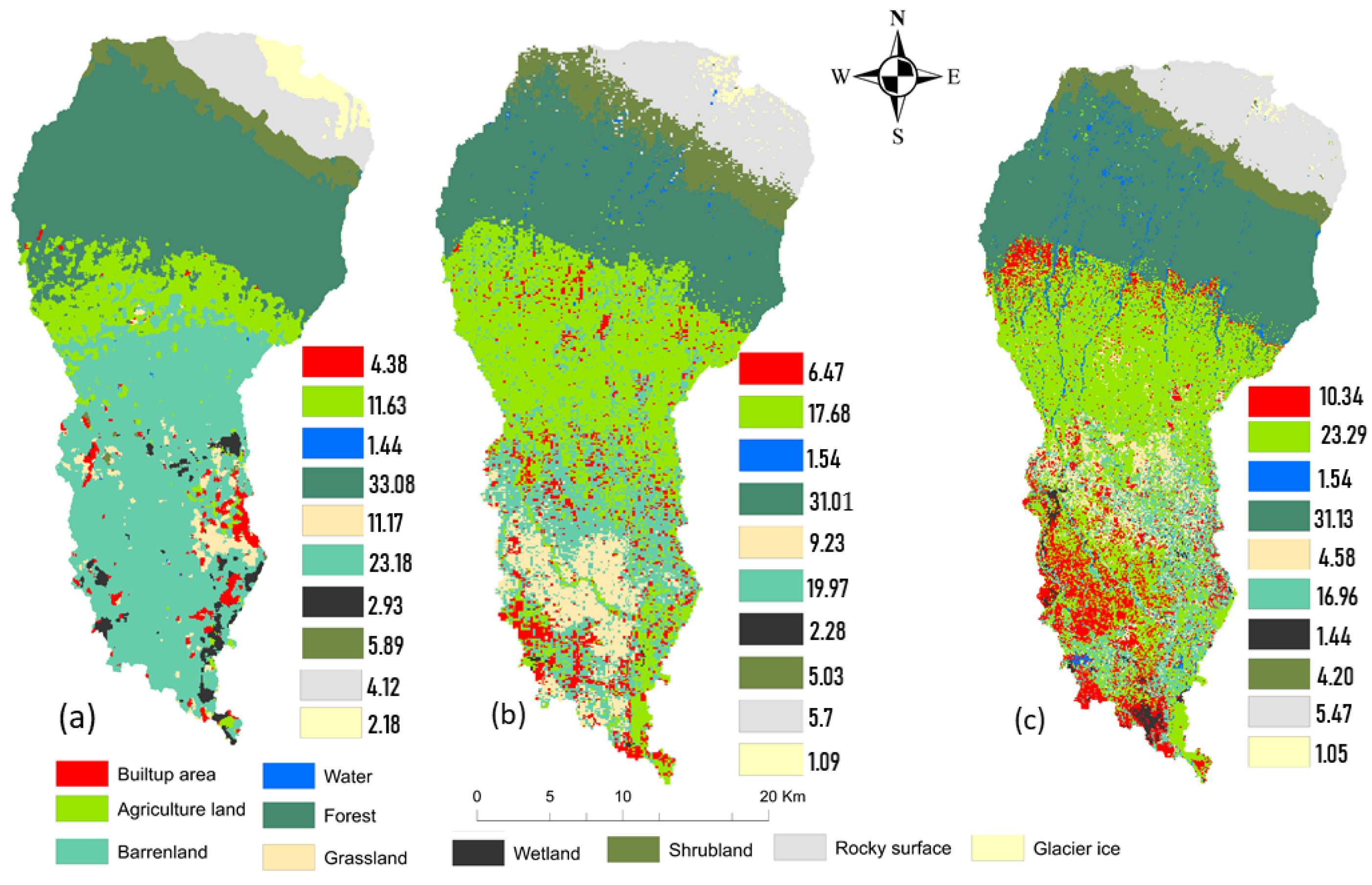
| LU | BULT | AGRL | WATR | FORR | BARR | GRSL | WTL | SHRL | SurfQ | LatQ | GWQ | ET | WatQ |
| 1993 | 4.38 | 11.63 | 1.44 | 33.08 | 11.17 | 23.18 | 2.93 | 5.89 | 295.39 | 38.86 | 168.93 | 502.0 | 513.00 |
| 2006 | 6.47 | 17.68 | 1.54 | 31.01 | 9.23 | 19.97 | 2.28 | 5.03 | 275.69 | 38.97 | 176.28 | 492.0 | 514.17 |
| 2018 | 10.34 | 23.29 | 1.54 | 31.13 | 4.58 | 16.96 | 1.44 | 4.20 | 345.23 | 36.3 | 205.91 | 471.2 | 672.29 |
| 2030 | 14.93 | 30.54 | 2.00 | 30.54 | 1.46 | 9.24 | 1.06 | 4.44 | 292.94 | 38.67 | 174.33 | 498.6 | 516.06 |
| Response Variable Y | Variation in Response | Q2 | Comp | Explained Variation in Y (%) | Cum Explained Variation in Y (%) | Root Mean PRESS | Q2 Cum |
|---|---|---|---|---|---|---|---|
| Hydrological components (ET, WatQ, SurfQ, GWQ, LatQ) | 0.951 | 0.901 | 1 | 94.1 | 94.1 | 0.272 | 0.9953 |
| 2 | 2.7 | 96.8 | 0.432 | 0.9926 | |||
| 3 | 1.8 | 98.6 | 0.561 | 0.9937 | |||
| 4 | 1.4 | 100 | 0.624 | 0.9481 |
| Variables | BUILT | AGRL | WATR | FORR | BARR | GRASL | WETL | SHR | ET | SurfQ | WatQ | GWQ | LatQ |
|---|---|---|---|---|---|---|---|---|---|---|---|---|---|
| BUILT | 1.00 | ||||||||||||
| AGRL | 0.98 | 1.00 | |||||||||||
| WATR | 0.80 | 0.89 | 1.00 | ||||||||||
| FORR | −0.74 | −0.85 | −0.99 | 1.00 | |||||||||
| BARR | −0.99 | −0.97 | −0.76 | 0.69 | 1.00 | ||||||||
| GRASL | −0.98 | −1.00 | −0.89 | 0.85 | 0.97 | 1.00 | |||||||
| WETL | −0.99 | −0.99 | −0.85 | 0.80 | 0.99 | 0.99 | 1.00 | ||||||
| SHR | −0.98 | −0.99 | −0.89 | 0.85 | 0.97 | 1.00 | 0.99 | 1.00 | |||||
| ET | 0.89 | 0.79 | 0.44 | −0.35 | −0.92 | −0.79 | −0.84 | −0.79 | 1.00 | ||||
| SurQ | 0.94 | 0.86 | 0.54 | −0.46 | −0.96 | −0.86 | −0.90 | −0.86 | 0.99 | 1.00 | |||
| WtrQ | 0.94 | 0.85 | 0.54 | −0.45 | −0.96 | −0.86 | −0.89 | −0.86 | 0.99 | 1.00 | 1.00 | ||
| GWQ | 0.99 | 0.94 | 0.69 | −0.62 | −0.99 | −0.94 | −0.97 | −0.94 | 0.95 | 0.98 | 0.98 | 1.00 | |
| LatQ | 0.94 | 0.86 | 0.54 | −0.46 | −0.96 | −0.86 | −0.89 | −0.86 | 0.99 | 1.00 | 1.00 | 0.98 | 1.00 |
| Variable | VIP | w*1 | w*2 | w*3 |
|---|---|---|---|---|
| BUILT | 1.28 | 0.316 | −0.878 | 0.444 |
| AGRL | 1.57 | 0.445 | −0.597 | −0.449 |
| WATR | 0.69 | −0.374 | −0.742 | −0.491 |
| FORR | 0.89 | −0.465 | 0.371 | 0.913 |
| BARR | 1.13 | −0.325 | −0.410 | −0.337 |
| GRAL | 1.10 | −0.386 | 0.324 | 0.493 |
| WETL | 0.65 | −0.206 | −0.236 | −0.3530 |
| SHRL | 1.11 | −0.228 | −0.264 | −0.4818 |
Publisher’s Note: MDPI stays neutral with regard to jurisdictional claims in published maps and institutional affiliations. |
© 2021 by the authors. Licensee MDPI, Basel, Switzerland. This article is an open access article distributed under the terms and conditions of the Creative Commons Attribution (CC BY) license (https://creativecommons.org/licenses/by/4.0/).
Share and Cite
Said, M.; Hyandye, C.; Mjemah, I.C.; Komakech, H.C.; Munishi, L.K. Evaluation and Prediction of the Impacts of Land Cover Changes on Hydrological Processes in Data Constrained Southern Slopes of Kilimanjaro, Tanzania. Earth 2021, 2, 225-247. https://0-doi-org.brum.beds.ac.uk/10.3390/earth2020014
Said M, Hyandye C, Mjemah IC, Komakech HC, Munishi LK. Evaluation and Prediction of the Impacts of Land Cover Changes on Hydrological Processes in Data Constrained Southern Slopes of Kilimanjaro, Tanzania. Earth. 2021; 2(2):225-247. https://0-doi-org.brum.beds.ac.uk/10.3390/earth2020014
Chicago/Turabian StyleSaid, Mateso, Canute Hyandye, Ibrahimu Chikira Mjemah, Hans Charles Komakech, and Linus Kasian Munishi. 2021. "Evaluation and Prediction of the Impacts of Land Cover Changes on Hydrological Processes in Data Constrained Southern Slopes of Kilimanjaro, Tanzania" Earth 2, no. 2: 225-247. https://0-doi-org.brum.beds.ac.uk/10.3390/earth2020014