
Evaluating Scaling Frameworks for Multiscale Geomorphometric Analysis


1
Department of Geography, Environment & Geomatics, University of Guelph, 50 Stone Road East, Guelph, ON N1G 2W1, Canada
2
Department of Geography, West University of Timisoara, 4 Vasile Parvan Boulevard, 300322 Timisoara, Romania
*
Author to whom correspondence should be addressed.
Geomatics 2022, 2(1), 36-51; https://0-doi-org.brum.beds.ac.uk/10.3390/geomatics2010003
Submission received: 25 November 2021
/
Revised: 24 December 2021
/
Accepted: 31 December 2021
/
Published: 2 January 2022
Abstract
:Multiscale methods have become progressively valuable in geomorphometric analysis as data have become increasingly detailed. This paper evaluates the theoretical and empirical properties of several common scaling approaches in geomorphometry. Direct interpolation (DI), cubic convolution resampling (RES), mean aggregation (MA), local quadratic regression (LQR), and an efficiency optimized Gaussian scale-space implementation (fGSS) method were tested. The results showed that when manipulating resolution, the choice of interpolator had a negligible impact relative to the effects of manipulating scale. The LQR method was not ideal for rigorous multiscale analyses due to the inherently non-linear processing time of the algorithm and an increasingly poor fit with the surface. The fGSS method combined several desirable properties and was identified as an optimal scaling method for geomorphometric analysis. The results support the efficacy of Gaussian scale-space as a general scaling framework for geomorphometric analyses.
1. Introduction
Many environmental processes interact with the Earth’s surface in complex ways to produce spatial distributions of landscape phenomena [1]. Topography is described mathematically as a closed, continuously differentiable two-dimensional manifold in three-dimensional Euclidean space [2]. Geomorphometry is the field of study concerned with the quantitative description of the Earth’s surface [3] using topographic data consisting of measurements of the three-dimensional location of the Earth’s surface. These measurements are used to create digital models of the surface given the sampling density and areal coverage, referred to individually as spatial resolution and extent respectively, and collectively as scale [4].
One of the primary functions of geomorphometry is characterizing topographic properties as land-surface parameters (LSPs, e.g., spatial distributions of slope, orientation, curvature, roughness, etc.) from the quantitative analysis of digital elevation models (DEMs) [5]. LSPs describe the morphology of the land surface using geometric and statistical, as well as application-specific measures [6]. Because the scaling resolution and extent are parameterized prior to LSP analyses, nearly all LSPs have well documented scale-dependency (e.g., [7,8,9,10,11]). Several application domains have demonstrated how scale-dependency propagates through analyses to affect results [12,13,14]. This is problematic because these scaling variables are first determined by sampling frameworks rather than the topography or phenomenon [15], providing a strong rationale for the integration of multiscale analysis in geomorphometry. Moreover, the relationship between scale and LSP measurement extends beyond the sampling framework and the surface generalization it imparts. The scale at which an LSP is measured specifies which landforms and processes are being measured [16]. Without a priori knowledge to narrow scale selection, all scales must be approached as potentially relevant.
Several families of scaling techniques have been devised to manipulate scale in geospatial analysis [4], many of which have direct application to geomorphometry. A direct approach to scaling involves manipulating the data resolution by predicting values at new locations, as if sampled with different spacing. The performance characteristics of this paradigm are largely determined by the quality and suitability of the predictive function (e.g., nearest neighbor, bilinear interpolation, kriging), and a large body of research exists comparing specific methods (e.g., [17,18]). Another approach involves manipulating the extent of the analysis, whether by a process-specific boundary such as a watershed, or by using local subsets of data defined by a neighborhood (e.g., [8,10,19,20]). Spatial filtering is particularly important because some LSPs are defined in terms of a local area, either by data requirements (e.g., finite difference methods), or by definition (e.g., topographic position). Spectral methods manipulate resolution by operating in the frequency domain, either through spatial filters [21,22] or wavelets [23]. Other scaling methods have been proposed, such as critical point selection methods for triangulated irregular network (TIN) data structures [24] or high-order polynomial approximation [25].
The variety of scaling approaches introduces a complex optimization process on practitioners in order to make informed decisions regarding method selection. The choice of approach and implementation impose limitations on study design by changing data parameters (e.g., changing cell size), restricting which LSPs are computable with a given methodological approach (e.g., [26]), or affecting the feasibility of computation. Processing time requirements are a subtly important consideration for multiscale analyses because non-linear processing time combined with the analysis of a continuous scale dimension is often time prohibitive [27], introducing a tradeoff between analysis quality (i.e., the density of scale sampling) and feasibility. Research comparing implementations and methods of the same framework (e.g., different interpolators) is abundant; however, there is little guidance to support decision making between the different scaling frameworks given the nuances and implications on study design. Understanding the performance tradeoffs of the scaling frameworks improves the ability to identify optimal methodological approaches for a given research objective.
This research aims to evaluate the merits of the various raster-based families of scaling frameworks for multiscale geomorphometric analyses. A multiscale analysis exploring different theoretical approaches and comparing each method’s outputs reveals the complex and nuanced relationships between approaches to scaling that guide experimental design. An ideal scaling framework should (1) maintain the spatial characteristics of the source data, (2) have a continuous scale parameter, and (3) have a relatively low computation time. The first criterion guards against spatial information loss, which introduces uncertainty due to the reduced ability to position a sample accurately in continuous space [20]. More specifically, maintaining spatial resolution allows the measurement of larger topographic structures without the need to coarsen the sampling interval. The second criterion ensures that the discretization of the scale dimension is as fine as the analysis requires rather than being imposed by methodological limitations (e.g., odd integers). The third criterion ensures that the framework is fast enough to apply to an arbitrary number of scales, allowing a scale-space sampling density suitable to the phenomenon under investigation. A constant time implementation of Gaussian scale-space is introduced to geomorphometry as a favorable general solution for multiscale analyses.
2. Background
This section provides an overview of the scaling frameworks and specific methods representing the framework. Three resolution-based methods (direct interpolation (DI), cubic convolution resampling (RES), and mean aggregation (MA)), one spatial filtering method (local quadratic regression (LQR)), one spectral method (fast Gaussian scale-space (fGSS)), were used to examine the properties of common raster-based scaling approaches in geomorphometry. A summary of the theoretical properties of each of the tested scaling methods evaluated in this research is given below (Table 1).
2.1. Resolution Methods
Resolution methods manipulate scale by changing the spatial support of the data. Spatial support refers to the geometry of the measurement units [28], which is the spatial resolution in the case of a regular gridded raster. This is achieved with the raster data structure by predicting values at unknown locations from known values using some predictive function, such as the interpolators used in the DI and RES methods, or by aggregating data into larger spatial units as exemplified by the MA method. Other data structures can also use resolution-based scaling by manipulating data density, such as the selection of points in a TIN data structure [29]. Because resolution methods achieve scaling by directly modifying the sample distance, they all modify spatial support by definition. Interpolators can scale continuously (i.e., they have a continuous scale parameter) because they predict values at arbitrary spacing. However, selecting a suitable interpolator is an important consideration because they are a known source of error [30]. Many predictive functions have been used, including simple linear interpolation [18], kriging methods [31], and more recently machine learning methods [32]. Aggregation summarizes sub-units into a spatially aggregated unit [33], thus the scaling is not continuous and is limited to integer multiples of aggregation units.
The DI method used in this research produces a raster grid via the linear interpolation of the triangular facets of a TIN generated by the Delaunay triangulation of LiDAR points. The RES method used cubic-convolution interpolator to resample existing raster grids to the specified sample spacing. DI and RES use different predictive functions (linear and cubic) applied to different data structures (TIN and raster) to generate regular gridded rasters of elevation at grid spacing (r). The DI and RES methods have constant processing times as neither interpolator varies with r. The MA method aggregates raster cells using an aggregation factor (a), to compute the mean of a neighborhood of a2 cells. The MA method typically has non-linear processing time as increasingly large mean filters are required; however, the tested MA method implemented the same constant time integral image-based mean filter as in [27].
2.2. Spatial Filtering
Spatial filtering is a convolution operation, where the spatial filter is the convolution kernel acting on the matrix of rasterized elevation values [34]. Spatial filtering methods manipulate scale by relating the size of convolution matrix to the spatial resolution of the underlying raster, allowing the manipulation of the areal extent of an analysis. While a spatial filter can be any shape or size, they are commonly used in geomorphometry to define a symmetrical, rectangular neighborhood around a center cell, which defines the spatial extent of the values included in the convolution function. Because the convolution is applied independently to every cell, the spatial resolution remains unchanged by the convolution operation. The symmetrical geometry of the convolution kernel limits possible filter sizes to odd integer values, thus limiting possible scales to odd integer multiples of r. Similar to resolution methods, the quality of the output and processing time both depend on the analytical function applied by the kernel, however, naïve filtering approaches increase exponentially with the filter edge length. Research in the field of computer vision has focused on improving the computational performance of filtering methods, often by accounting for redundancy in overlapping kernels (e.g., [35]). Some of these methods were evaluated in [26].
The LQR method uses a convolution kernel that applies a least-squares fitting scheme to solve the coefficients of a bivariate quadratic equation (Equation (1)). Several local derivatives, including slope (s) and profile curvature (cprof), as defined in [36], are computed once the six coefficients of the paraboloid (a, b, c, d, e and f) are known (Equations (2) and (3); taken from [20]). Equation (3) has been multiplied by 100 to express curvature as a percent gradient per unit length.
where x and y are the coordinates of a spatial position.
This system of equations can be expressed as a 6 × 6 matrix solving for each the coefficients of the paraboloid using local elevation values as defined by the spatial filter. Expressing all elevation samples in the convolution kernel as relative vertical changes and constraining the constant f to the origin of the central cell (i.e., f = 0) results in an exact predictor at the origin (Equation (4)) [20]. This simultaneously simplifies matrix operations by removing the last row of the matrix and associated vectors, and improves the estimated local derivative by forcing the surface to travel through the origin of the central cell.
where i is a sample in the convolution kernel and zi is the difference in elevation between the sample and the center cell.
2.3. Spectral Methods
Spectral methods manipulate topographic signals in the frequency domain rather than the spatial domain (though often implemented in the spatial domain). Scale-space theory was developed in the 1980s in the field of computer vision to address scaling in images [37,38]. Scaling was modelled as the diffusion of brightness in an image using the Gaussian function as a solution to the heat diffusion equation [39]. The theory stipulates that scale-space implementations use linear and shift-invariant operators, have a continuous scale parameter, and that the structure within the input image should monotonically disappear as scale is coarsened [40]. The constraint that fine structure disappears inversely to scale preserves the signal of progressively larger scale features; a process that has been described as “lifting off detail” [37]. Convolution using a bivariate Gaussian function Equation (5) was quickly recognized to satisfy the axioms of scale-space theory and was proven to be uniquely suitable [41,42].
where x and y are coordinates in two-dimensional space and g is the standard deviation.
Despite the clear application for Gaussian scale-space in geomorphometry, it has seen little application in the field largely due to the prohibitively high computation times at large scales. Working in the field of computer vision, [43] published a Gaussian kernel approximation method that achieved a small and fixed computational cost irrespective of the filter size based on repeated mean filtering. This implementation reduces processing time requirements significantly, remaining constant with increasing scale rather than the usual increase in computation.
2.4. Recursive Methods
Recursion-based scaling itself is not a scaling framework, but an implementation of a scaling framework. While recursion is too large of a topic to cover adequately, in the context of this research recursive methods are defined as the re-application of some scaling operation to its own output until some stopping condition is reached. This is meant to differentiate recursive implementations from the common approach of iteratively modifying a scaling parameter (e.g., [8,10,44]). Recursion is well-known in region-growing image segmentation (e.g., [45]) because it forms strict hierarchies of objects at different scales. Region-growing image segmentation is at the core of geographic object-based image analysis (GEOBIA) [46] and has been applied to geomorphometric analyses [44,47], although not in a strictly recursive sense. Other recent examples of recursive methods in geomorphometry include discrete wavelet decomposition [48,49] and Gaussian pyramiding [50].
Gaussian pyramiding is scale-space implementation originally developed to rapidly generate multiscale representations of visual information [51]. Gaussian pyramids leverage down-sampling and cascaded Gaussians to reduce data volume and filter sizes while simultaneously minimizing aliasing artifacts [52]. First a low-pass Gaussian convolution is applied to remove high-frequency information from the signal, followed by the decimation of samples rendered redundant by the smoothing filter. These two operations are repeated, successively blurring and resampling the image, using the rescaled output image as the input to the next iteration until there are too few samples to repeat the process. The recursive implementation of Gaussian smoothing differs from an iterative approach described above (Section 2.3) in that sigma values are fixed, effectively limiting scale intervals to > [52]. The rather coarse scale sequence and rapid reduction in data volume enables short computation time for the full range of scales supported by the number of samples. Up-sampling back to the original resolution is possible using the same Gaussian function as the interpolator [50]. A more detailed description of the original approach (a Laplacian pyramid) developed for image processing is found in [53]. Konlambigue et al. [54] have implemented a Gaussian pyramid using a similar mean filter approximation method as [43], resulting in comparable computational efficiency.
3. Materials and Methods
3.1. Study Site and Source Data
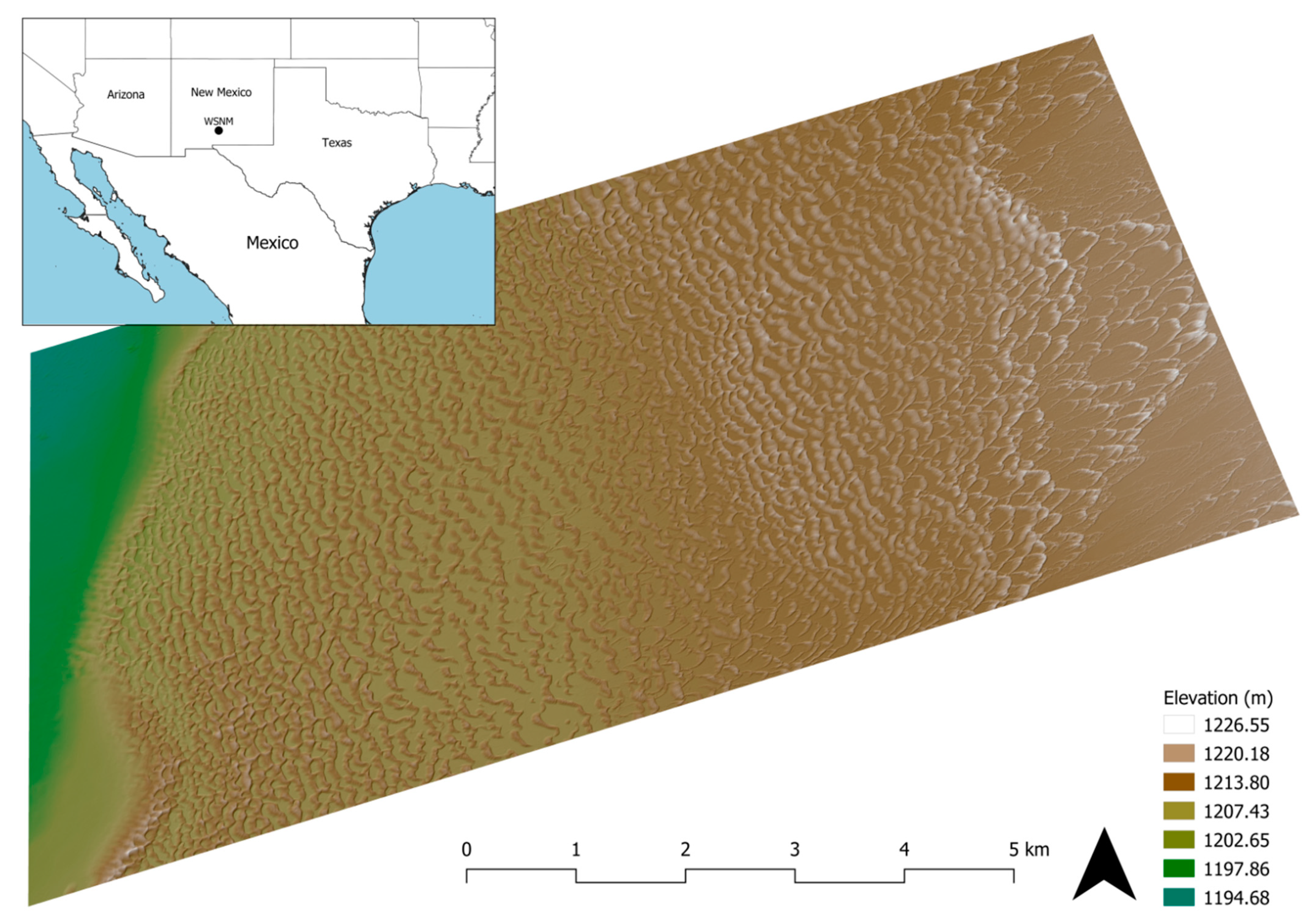
This research used a LiDAR data set covering ~47 km2 of the sand dune field at White Sands National Monument (WSNM), approximately 40 km west of Alamogrodo, New Mexico, USA (North: 32.872402°, South: 32.795823°, East: −106.186273°, West: −106.314333°) (Figure 1). The site is located to the east of a large, aerodynamically smooth gypsum flat, where aeolian processes have formed a large dune field [55]. The dune ridges are generally oriented along the north-south axis until approximately 7000 m east of the margin between the flat and the dune field (~7000 m downwind of the upwind margin), where the dunes transition from crescentic and barchan dunes to parabolic dunes [55,56]. The crest spacing (i.e., wavelength) increases from 80 m to 150 m and crest heights decrease from 14 m to 8 m along the west-to-east gradient [55]. Furthermore, the site has very low relief with an elevation range for the entire data set less than 32 m.
The data were collected on 24 January 2009 by the National Center for Airborne Laser Mapping (NCALM) with a point density of 5.25 points/m2 and a vertical RMS of 0.041 m between control points and the nearest LiDAR point [57]. A ground point filter was used to remove off-terrain objects. A baseline 2-m resolution DEM was generated by applying the DI method to the LiDAR point cloud.
3.2. Comparing Scales
Because the resolution, spatial filtering, spectral, and recursive scaling approaches use fundamentally different methods and parameters to manipulate scale (i.e., resolution, neighborhood size, spectra respectively), a consistent quantification of scale was required to facilitate comparisons across methods. Let λ be a parameter that represents the shortest theoretical wavelength in the elevation field resulting from the application of a scaling method. This describes the reduction in the apparent detail by limiting the ability to characterize topographic wavelengths below λ. Let a scaling operation be a function that maps a method-specific scale parameter (p) to the λ of the output (Equation (6)).
The scale parameter for resolution methods is the resolution of the data (r), which is a regular spatial sampling interval. The Shannon–Nyquist sampling theorem states that “to keep features with a wavelength, a resolution less than or equal to half of the wavelength is required [to reconstruct the continuous function]” [30] (p. 482), or formally, , assuming rx = ry. λ can be defined in terms of r by rearranging the sampling theorem and expressed in units of length, and thus any scaling operation that manipulates r takes the form
where is a method of manipulating the resolution of a DEM such that the output has resolution r.
Note that the Shannon–Nyquist sampling theorem applies specifically to the resolution that the elevation field was sampled at rather than the resolution property of the DEM. While these two are the same thing prior to any scaling operation, there is a one-way information loss as scale is increased such that information is lost even if data are down-sampled back to the original resolution.
Spatial filtering methods use the filter size as the scale parameter. The spatial characteristics of a filter can be described by the number of cells along the filter edge (L) assuming Lx = Ly. The large flexibility of filter functions makes general statements about the relationships between scaling and filter size difficult. In the case of the LQR method, the information within the extent of the filter is analyzed by the filter function, or more specifically the elevation samples are used to model a continuous parabolic surface from which measurements are made. This particular case of spatial filtering does not manipulate the scale of the elevation field, but the scale at which a LSP is measured. Because the paraboloid can only have one extremum in each dimension, the smallest wavelength the parabolic surface can model is length rL. Wavelengths between the resolution of the data and this length cannot be reproduced by the model and presents as a poor fit between the paraboloid and the underlying elevation samples.
Gaussian smoothing is used as the example of spectral smoothing, where smoothing in frequency domain results in the attenuation of high frequencies. Because the Fourier transform of a Gaussian function is another Gaussian function, the standard deviation parameter in the standard deviation in the frequency domain (gf) is related to the standard deviation in the spatial domain (g) by:
A cut-off frequency (fc) can be defined to identify a frequency such that greater frequencies are weighted sufficiently low by the Gaussian function (Equation (10)). For example, the field of computer vision commonly uses the frequency at half amplitude as cut-off frequency because frequencies beyond ln(2) × gf are weighted ≤0.5.
where w is the frequency response of the filter.
The reciprocal of the shortest wavelength corresponds to the largest frequency, which when equated to fc allows λ to be expressed in terms of g:
3.3. Evaluation
Four experiments were conducted to empirically evaluate the performance of each scaling method. First a sequence of 14 target λ ranging from 6 m to 318 m was used to generate theoretically comparable outputs for each scaling method. The upper limit of the target λ range exceeds the largest dune crest spacing and is therefore sufficiently large to observe the loss of topographic detail in the data set (i.e., the dunes are no longer expressed). A w value was selected for the fGSS such that the cut-off frequency was three standard deviations in the frequency domain, where frequencies above this cut-off are reduced by approximately 99.73% (i.e., are weighted 0.0027). Slope (s) and profile convexity (cprof) were derived for all DEM outputs (i.e., the resolution methods and fGSS method) using the LQR method using the minimum filter size of three cells (see Section 2.2 for details). The scaling effect of this additional LQR measurement is ignored because a neighborhood of at least 3 × 3 is required to compute the local derivatives. Thus, a LQR filter size of 3 is exclusively considered a measurement, while larger filters were evaluated as scaling operations. Restricting LSP generation to the LQR method also restricts the interpretation of scaling operations to the impact on the topographic surface, rather than the LSP formulation.
Second, the processing time of each scale and method was recorded to evaluate processing time requirements. The DI method required the interpolated rasters mosaicked together to form the final raster at every scale. The sum of the execution time of DI and mosaic operations was recorded as execution time since both operations were required for the LiDAR tiles. However, this only affects the absolute processing time rather than the time complexity order since the number of tiles being mosaicked is constant across scales and is specific to the data set. A rigorous benchmark was not necessary because the variation in runtime for a method-scale pair was small, and the differences between methods are generally large.
Third, empirical quantile-quantile plots comparing scaled DEMs and LSPs to the baseline counterparts were generated to examine how each scaling method modifies distributions across scales. The deviation from the initial distribution (represented by the 1:1 line) shows the changes imparted by the scaling operation. A linear regression was conducted to model QQ-plot distributions for each scale to quantify the effect of each scaling operation. The coefficient of the linear model compares the distributions of the base example and scaled counterpart as a ratio where a coefficient of 1 lies on the 1:1 line of the QQ-plot, and implies no change to the distribution as a result of the scaling operation. Finally, a goodness-of-fit analysis was conducted on the LQR method to investigate how well the paraboloid fit the surface at each location across the range of scales. This analysis quantifies how the modeled surface responds to changes in the filter size. All tested methods used parallel processing implementations wherever possible and were integrated into the WhiteboxTools software environment [58].
4. Results
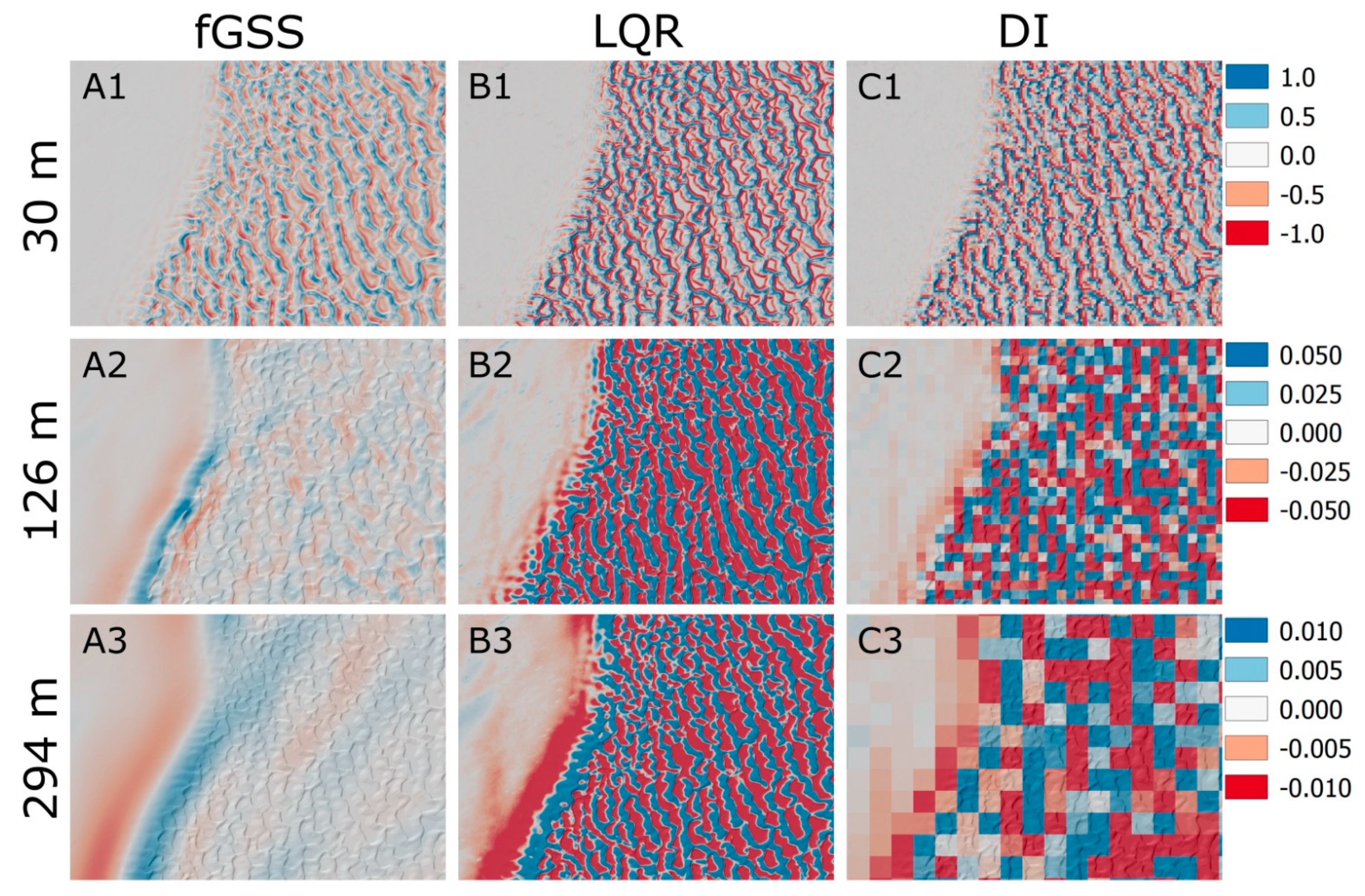
The multiscale analysis conducted on the WSNM site generated a sequence of scaled outputs for each method, defined in terms of λ. The LQR method was applied to the smoothed elevation outputs to generate slope (s) and profile convexity (cprof) spatial distributions. Figure 2 shows a subset of output rasters to demonstrate the differences in cprof outputs between scales and methods represented as rows and columns respectively. The scale rows were chosen to demonstrate outputs far below (λ = 30 m), near (λ = 126 m), and far above (λ = 294 m) the dune crest spacing distances found in the site description. The methods are hardly distinguishable at 30 m scale (Figure 2(A1,B1,C1)), although the fGSS method produced lower magnitude values. At the 126 m scale (Figure 2(A2,B2,C2)) the fGSS method diverges from the other methods, with vast areas of the site possessing values near zero, while LQR and DI methods remained very similar, with the latter retaining more detail in flat areas. At 294 m (Figure 2(A3,B3,C3)), the fGSS method (Figure 2(A3)) showed only large curvature structures, effectively minimizing the impact of the dune topography on the cprof values. The LQR method (Figure 2(B3)) shows the same large-scale structure at the margin between the gypsum flat and the dune field as the fGSS method; however, it also retained much information from smaller dunes. The DI method (Figure 2(C3)) exhibits a spatial pattern similar to the LQR method. However, the large cell sizes obscure the relationship between cprof value and the underlying topography such that the topographic geometry driving the measured curvature value is unknown. The RES and MA methods are not shown due to the visual similarity to the DI method. However, RES and DI differed slightly when presenting the spatial pattern of dune structures. MA followed the spatial pattern of DI more closely, but presented curvature values at smaller magnitudes relative to DI.
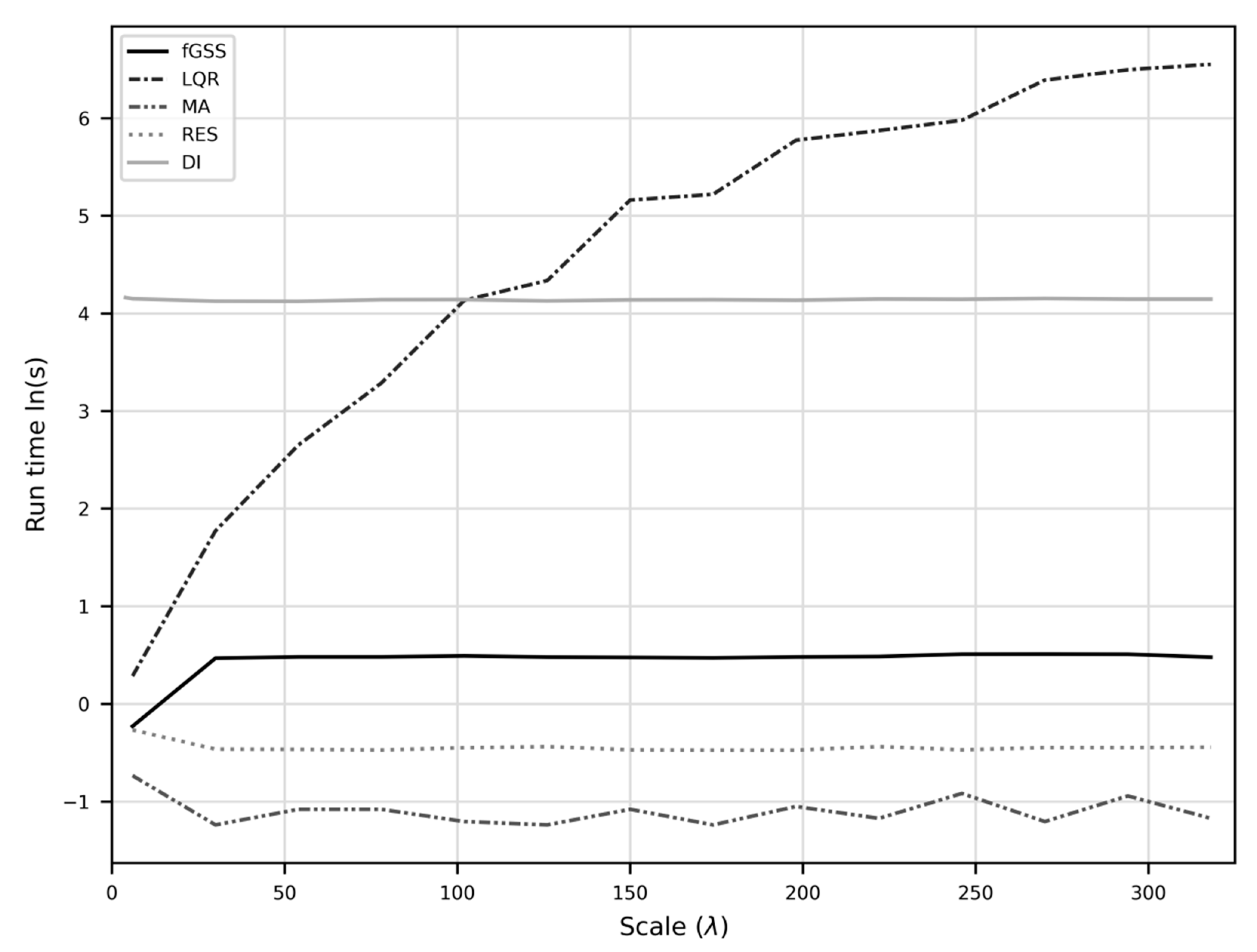
The processing time analysis showed scale-independent processing time requirements for all methods except LQR, which had non-linear processing time (Figure 3). The fGSS method was scale independent due to the fast Gaussian approximation implementation, requiring 1.5 s per scale on average. The first scale required less time than the rest due to a minimum standard deviation limitation of the fast implementation, below which a standard Gaussian filter must be used. The LQR method took exponentially longer as scale increased, requiring over 700 s at the end of the experimental range. The DI method was relatively slow due to the additional mosaic operation required to combine the rasterized LiDAR tiles; however, the TIN gridding operation alone required less than 10 s for all scales. The MA and RES methods were the fastest, with both consistently completing in under a second.
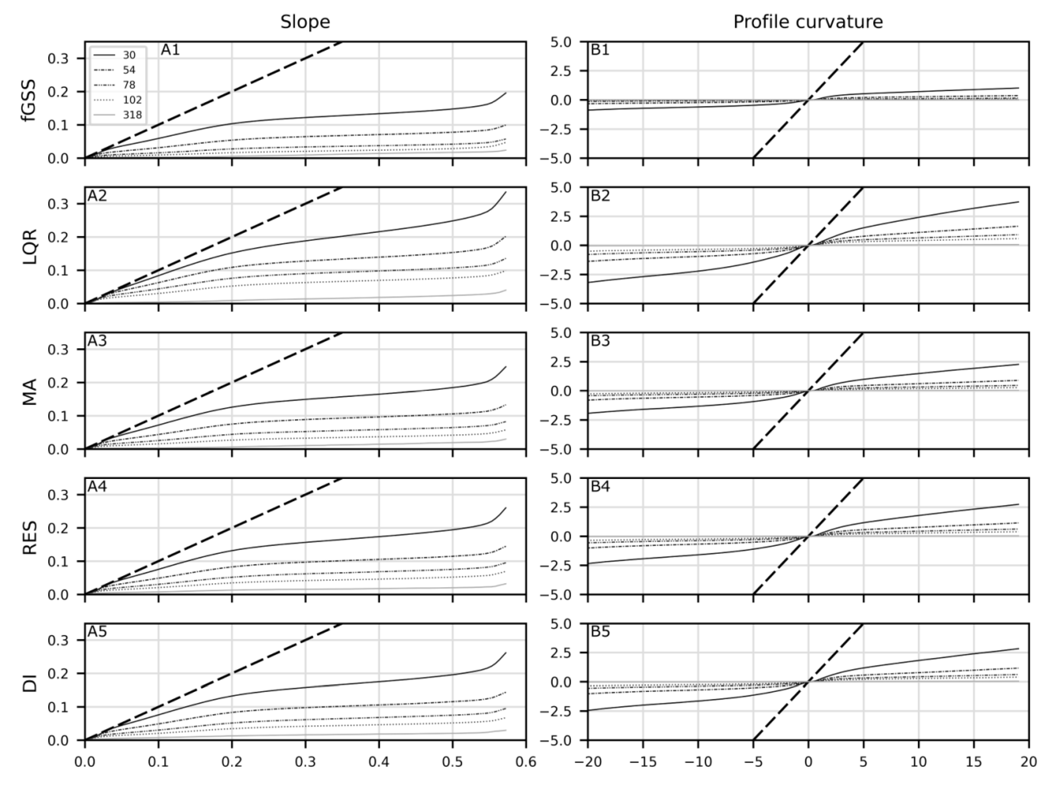
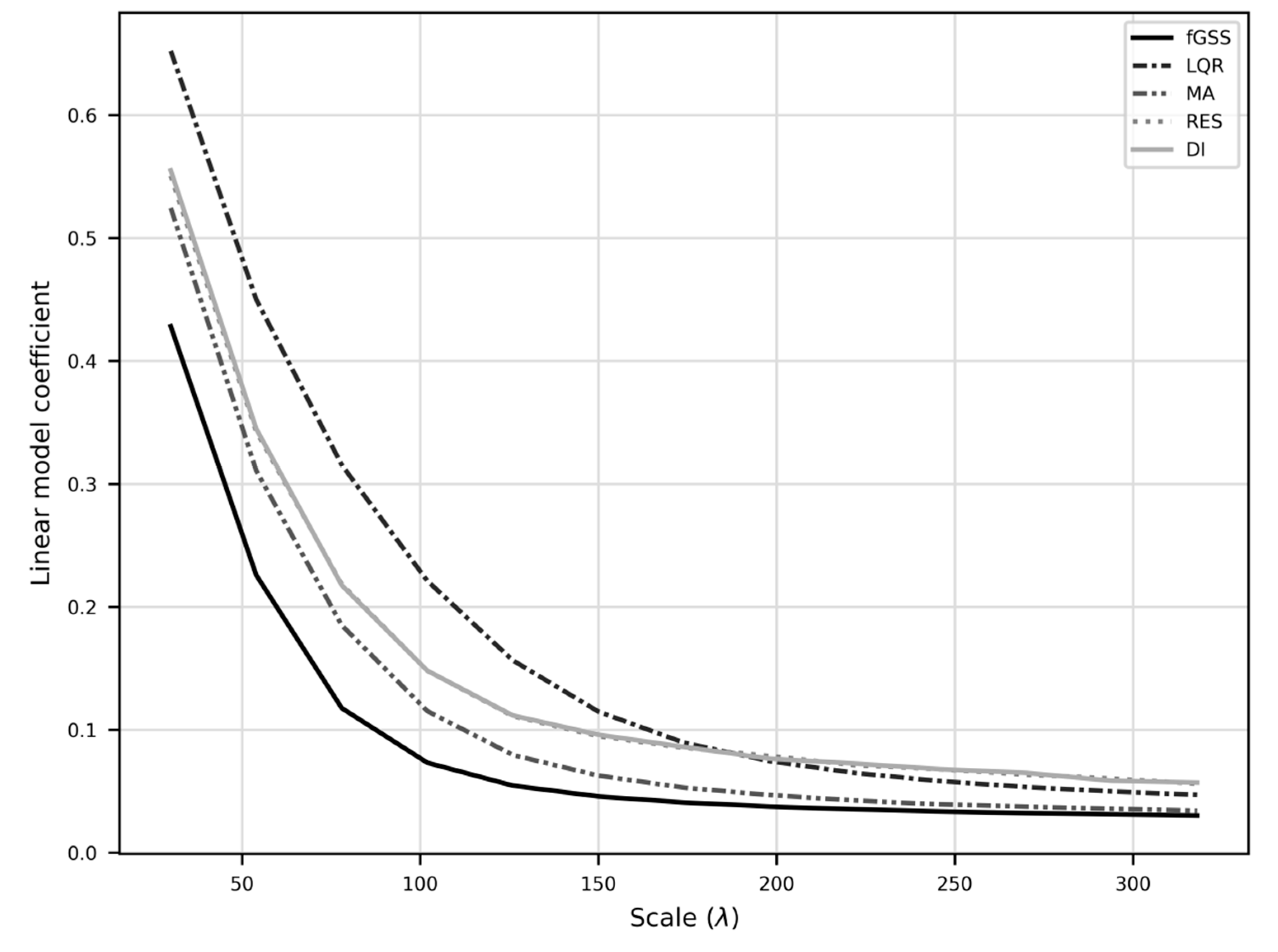
The scaled elevation and local derivative outputs were compared to a base line data set generated using the DI method to produce a base DEM with λ = 2 m using a 3 × 3 LQR filter to compute s and cprof distributions. Figure 4 shows a matrix of QQ-plots (n = 500) using the base line content as the theoretical distribution to demonstrate how the distribution is modified as scale increases for each method (rows 1 to 6) and s and cprof (columns A and B). All methods reduce the value of the output local derivatives, flattening all distributions towards zero as scale increases. Importantly, the shape of the modified distributions remains the same for all methods across scales. Figure 4B shows that fGSS modifies distributions the most aggressively, while the LQR and DI methods are the most conservative. Because the QQ-plot of the slope LSP closely follows a linear model, the coefficient of each linear model was plotted to approximate the degree to which each method generalized the slope distributions as a function of scale (Figure 5).
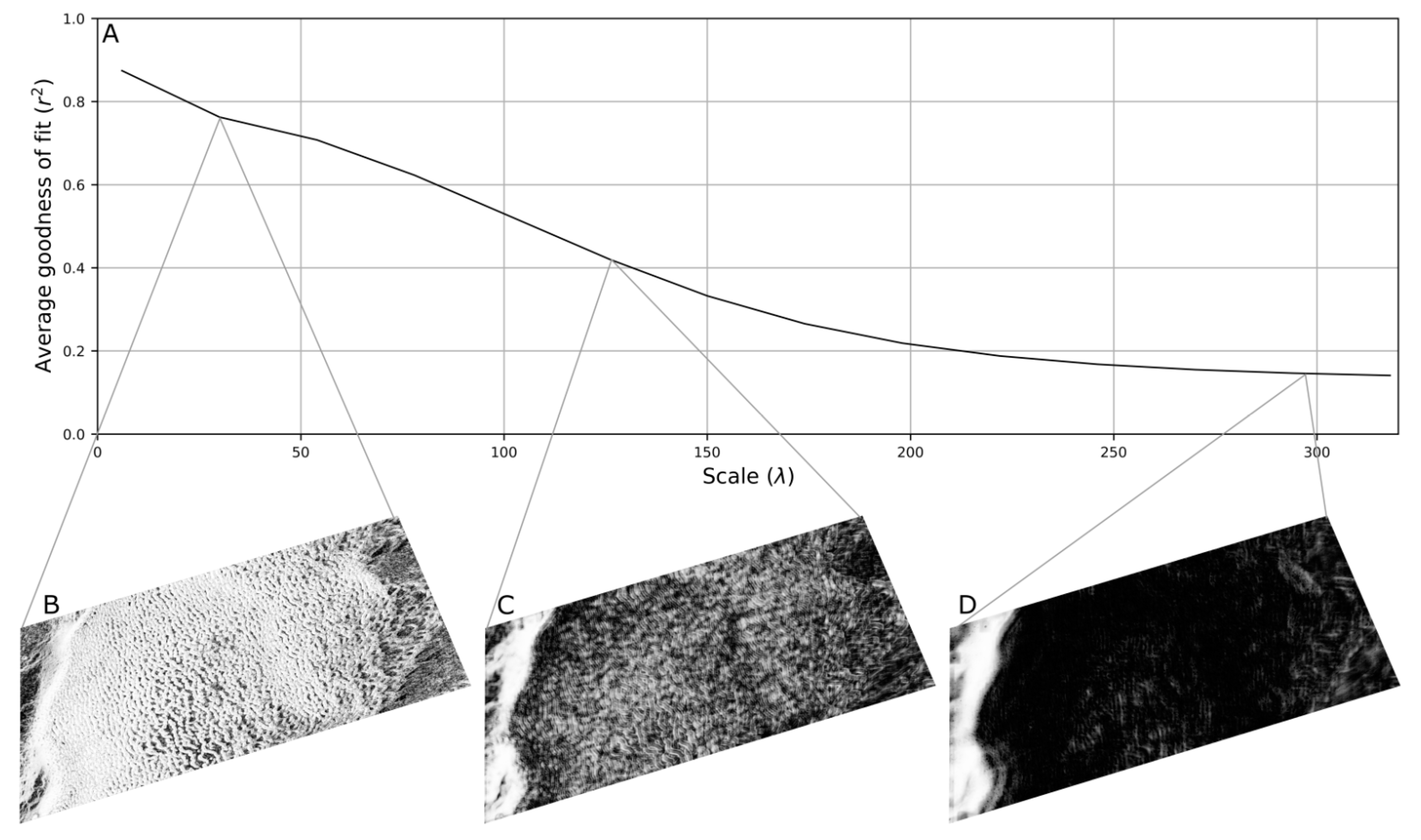
A goodness-of-fit analysis was conducted to determine the ability of the LQR paraboloid function to predict the landscape used to parameterize it. Figure 6A shows the raster wide average r2 value across scales, demonstrating a reasonably good fit at small scales (i.e., window sizes), which decreases as scale increases. Figure 6B–D shows that the gypsum flat on the left edge retains large goodness-of-fit values across all scales, while the dunes become almost entirely misrepresented by the model surface by 294 m.
The fGSS method produced a notable edge effect at the midpoint of the spatial filter. The effect is imperceptible in the elevation field, but becomes prominent when local derivatives are calculated. The fGSS method achieves computational efficiency using the integral image data structure, which was developed for images without consideration for ‘NoData’ values. Filling data holes during pre-processing and buffering the data edges is recommended for best results when using fGSS. It should also be noted that 32-bit precision was insufficient to store the fGSS output elevation data at large scales due to the high degree of generalization and very flat site.
5. Discussion
The results demonstrate that all methods modify the distribution predictably and to comparable degrees. All methods cause an exponential decay of information, with stronger effects on the extrema of the distribution (Figure 4 and Figure 5). While an in-depth analysis of error was not performed, significant systemic errors were not observed in the numerical distributions between methods and scaling frameworks. Despite the known errors from aggregation [15], the MA-scaled distributions are almost indistinguishable from those produced by RES and DI, aside from noticeably stronger generalization. The RES and DI methods modify the original distribution almost identically (Figure 5) despite being derived from raw LiDAR instead of the baseline raster. Grohmann [17] found that interpolating from source data or from fine-resolution raster is superior to interpolating from some intermediate data. The results support this statement insofar as it confirms that the differences between a linear TIN-based interpolator and a cubic grid-based interpolator are negligible. The similarities between resolution methods suggest that choice of predictive function has a minimal impact relative to the large impact of scaling. This agrees with previous findings that simple predictors are sufficient for DEM scaling [18].
The greatest weakness of resolution methods is the poor ability to interpret data values for increasingly large grid cells. This is observed in Figure 2 clearly, where the DI method begins with cells small enough to relate to the underlying topography and ends with a spatial distribution too coarse to infer topographic meaning, or differentiate signal from noise. This property hinders the utility of resolution methods for multiscale analysis and compounds with known errors associated with resolution manipulation [20]. Therefore, while resolution methods are competitive when deriving scaled global statistics, they are unsuitable if the preservation of localization information is desired. Choice in initial resolution is an important consideration when translating raw data into an elevation data product. Along with the increased detail captured by fine-resolution sampling come noise and measurement error. Recent advances in feature-preserving DEM generalization have addressed this weakness by selectively avoiding the generalization of topographic features while generalizing other areas [59,60]. Feature-preserving generalization methods are a promising option for pre-processing elevation data prior to analysis as they differentiate the application of generalization for de-noising from a scaling operation.
The tested spatial filtering method, LQR, achieves scaling by parameterizing a model paraboloid from elevation samples collected over larger areas [20]. As expected from the theoretical properties, the empirical results demonstrate the preservation of spatial resolution (Figure 2(B1–B3)) and non-linear processing time (Figure 3). LQR also altered the scaled distributions less than all other methods λ < 174 m, where RES and DI had less impact (Figure 5). However, the spatial distributions in Figure 2 demonstrate that LQR tends to retain detail regardless of the scale selected. Based on the results of [10], a stronger relationship between the window size and topographic structure was expected. For example, the cprof output at a scale of 294 m (i.e., a 147 × 147 cell filter, Figure 2(B3)) was expected to contain little information from the dune structure because λ exceeds even the largest dune wavelengths by a large margin. Yet many short wavelength dunes are well defined along with large scale topographic features such as the transition from the gypsum flat to the dune field (Figure 2(B3)). The unpredictable behavior from the filter size scaling parameter demonstrates an inability to target scales at which topographic features are known to exist, hindering utility as a method for scaling local derivative measurements. While increasing the filter size does indeed influence the geometric properties of the paraboloid, the relationship between filter size and the scale of the topography weakens as scale increases. The goodness-of-fit analysis in Figure 6A suggests that this is in part caused by an increasingly poor fit between the paraboloid and the underlying topography. The poor surface representation occurring at large scales coincides with the dune field, where the modeled surface lacks the flexibility to adopt the shape of the underlying terrain once multiple dune structures are within the filter extent (Figure 6D). The goodness-of-fit of the modelled surface effectively characterizes the mismatch between the scale of the analysis and scale of the topography, suggesting that measurement accuracy is degraded at large scale. Thus, while the spatial pattern appears to converge on a pattern representative of the underlying topography, both the relationship between the scale parameter and topography, and the accuracy of the measurement degrade rapidly as scale increases.
Empirical testing of the fGSS method confirms the maintenance of spatial resolution and constant processing time. The parameter w was set to e9/2 to ensure all frequencies above three standard deviations in the frequency domain were weighted near 0.0. However, this resulted in more aggressive smoothing of the distribution relative to the other scaling methods (Figure 4). This suggests that a smaller value such as the more conventional value of 2, meaning full width at half maximum in the frequency domain [43], would better calibrate the loss of detail relative to the other scaling methods. Despite the aggressive smoothing, the spatial distributions performed as expected, with information from small dunes being progressively removed as scale increased, leaving larger scale structures to dominate the spatial distribution (Figure 2(A1–A3)). The predictable control of the size of topographic structures being measured was not observed with the other methods, demonstrating strong potential for generalizing topography to represent scale-specific structure, which is an ideal property for multiscale topographic analysis.
While the fGSS method was developed to provide the flexibility to fully sample the scale dimension, this experimental design did not capitalize on the continuous scale parameter of fGSS beyond calibrating g to the other scaling parameters via λ. Similar scale-space implementations such as the recursive counterpart to fGSS, the Gaussian pyramid, are better optimized to provide increased efficiency at the expense of a far coarser ability to sample scales. Behrens et al. [50] proposed a modified Gaussian pyramid for terrain analysis using multiple starting points for improved scale discretization, which they termed extended Gaussian Pyramid (eGP). They examined the performance of different scaling methods, comparing spatial filtering with three other methods of deriving LSPs from the extended pyramid: ‘terrain scaling’ where LSP are calculated and then subjected to the pyramiding, ‘DEM scaling’ where the DEM is subjected to pyramiding, followed by the LSP calculation at the end, and ‘Mixed scaling’ where the LSP is calculated on the down-sampled DEM followed by up-sampling of the LSP. They found that mixed scaling provided the most accurate soil property predictions, and was improved by the use of intermediate scales. Progress made to improve the efficiency of Gaussian convolution, and to improve the scale discretization of Gaussian pyramids, has made the choice in Gaussian scale-space implementation for terrain analysis less vital. The results presented above together with [50] demonstrate the applicability of both implementations for multiscale geomorphometric analyses, where fGSS is advantageous when continuous scale sampling is desirable and time restrictions are relaxed.
6. Conclusions
This research sought to evaluate the merits of several scaling frameworks for general-purpose multiscale geomorphometric analyses. Resolution methods, spatial filtering, and spectral methods were compared in a multiscale analysis using local derivatives. Resolution methods, while ubiquitous and intuitive, share several undesirable properties, such as the modification of the spatial resolution resulting in the loss of spatial information. The tested resolution methods were fast and had a relatively small impact on the statistical distribution, and therefore may be useful for statistical analyses.
LQR is a spatial filtering method that maintains spatial resolution and has an intuitive scale parameter. However, the results exposed a weak relationship with the underlying topography where information is often retained across several scales. This relationship becomes weaker at larger scales, which when coupled with large processing time requirements, hinders utility as a multiscale framework.
Spectral methods have formed the theoretical basis for scaling image data. The fGSS method maintains spatial resolution, has a continuous scale-parameter, and is relatively efficient to compute; these are all desirable properties for multiscale analyses. While it aggressively modifies the distribution compared to the other tested methods, it produced a strong, predictable relationship between the scale parameter and landscape structure. Thus, the fGSS method proposed above addresses many shortcomings of spectral scaling and has many desirable properties for multiscale geomorphometric analysis. Gaussian scale-space, including fGSS, represents a general solution to topographic scaling.
Author Contributions
Conceptualization, D.R.N. and J.B.L.; Data curation, D.R.N. and J.B.L.; Formal analysis, D.R.N.; Funding acquisition, J.B.L.; Investigation, D.R.N.; Methodology, D.R.N.; Project administration, J.B.L.; Resources, D.R.N.; Software, D.R.N. and J.B.L.; Supervision, J.B.L., J.M.H.C. and L.D.; Validation, D.R.N.; Visualization, D.R.N.; Writing—original draft, D.R.N.; Writing—review & editing, J.B.L., J.M.H.C. and L.D. All authors have read and agreed to the published version of the manuscript.
Funding
This research was funded by a grant provided by the Natural Sciences and Engineering Research Council of Canada (NSERC; grant number 400317).
Institutional Review Board Statement
Not applicable.
Informed Consent Statement
Not applicable.
Data Availability Statement
Publicly available datasets were analyzed in OpenTopography at https://0-doi-org.brum.beds.ac.uk/10.5069/G97D2S2D (accessed on 22 May 2021).
Acknowledgments
LiDAR data acquisition and processing completed by the National Center for Airborne Laser Mapping (NCALM—http://www.ncalm.org) (accessed on 22 May 2021). NCALM funding provided by NSF’s Division of Earth Sciences, Instrumentation and Facilities Program. EAR-1043051.
Conflicts of Interest
The authors declare no conflict of interest. The funders had no role in the design of the study; in the collection, analyses, or interpretation of data; in the writing of the manuscript, or in the decision to publish the results.
References
- Moore, I.D.; Grayson, R.B.; Ladson, D.A.R. Digital Terrain Modelling: A Review of Hydrological, Geomorphological, and Biological Applications. Hydrol. Process. 1991, 5, 3–30. [Google Scholar] [CrossRef]
- Florinsky, I.V. An Illustrated Introduction to General Geomorphometry. Prog. Phys. Geogr. Earth Environ. 2017, 41, 723–752. [Google Scholar] [CrossRef]
- Pike, R.J. Geomorphometry: Progress, Practice and Prospect. Z. Fur Geomorphol. NF Suppl. 1995, 101, 221–238. [Google Scholar]
- Goodchild, M.F. Scale in GIS: An Overview. Geomorphology 2011, 130, 5–9. [Google Scholar] [CrossRef]
- Pike, R.J.; Evans, I.S.; Hengl, T. Geomorphometry: A Brief Guide. Dev. Soil Sci. 2009, 33, 3–30. [Google Scholar] [CrossRef]
- Olaya, V. Basic Land-Surface Parameters. In Developments in Soil Science; Elsevier Ltd.: Amsterdam, The Netherlands, 2009; Volume 33, pp. 141–169. [Google Scholar] [CrossRef]
- Deng, Y.; Wilson, J.P.; Bauer, B.O. DEM Resolution Dependencies of Terrain Attributes across a Landscape. Int. J. Geogr. Inf. Sci. 2007, 21, 187–213. [Google Scholar] [CrossRef]
- De Reu, J.; Bourgeois, J.; Bats, M.; Zwertvaegher, A.; Gelorini, V.; De Smedt, P.; Chu, W.; Antrop, M.; De Maeyer, P.; Finke, P.; et al. Application of the Topographic Position Index to Heterogeneous Landscapes. Geomorphology 2013, 186, 39–49. [Google Scholar] [CrossRef]
- Grohmann, C.H.; Smith, M.J.; Riccomini, C. Multiscale Analysis of Topographic Surface Roughness in the Midland Valley, Scotland. IEEE Trans. Geosci. Remote Sens. 2011, 49, 1200–1213. [Google Scholar] [CrossRef] [Green Version]
- Schmidt, J.; Andrew, R. Multi-Scale Landform Characterization. Area 2005, 37, 341–350. [Google Scholar] [CrossRef]
- Sørensen, R.; Seibert, J. Effects of DEM Resolution on the Calculation of Topographical Indices: TWI and Its Components. J. Hydrol. 2007, 347, 79–89. [Google Scholar] [CrossRef]
- Behrens, T.; Schmidt, K.; Ramirez-Lopez, L.; Gallant, J.; Zhu, A.X.; Scholten, T. Hyper-Scale Digital Soil Mapping and Soil Formation Analysis. Geoderma 2014, 213, 578–588. [Google Scholar] [CrossRef]
- Kumar, S.V.; Peters-Lidard, C.D.; Mocko, D. Multiscale Evaluation of the Improvements in Surface Snow Simulation through Terrain Adjustments to Radiation. Hydrometeorology 2013, 14, 220–232. [Google Scholar] [CrossRef]
- Sofia, G.; Pirotti, F.; Tarolli, P. Variations in Multiscale Curvature Distribution and Signatures of LiDAR DTM Errors. Earth Surf. Process. Landf. 2013, 38, 1116–1134. [Google Scholar] [CrossRef]
- Dark, S.J.; Bram, D. The Modifiable Areal Unit Problem (MAUP) in Physical Geography. Prog. Phys. Geogr. 2007, 31, 471–479. [Google Scholar] [CrossRef] [Green Version]
- Minár, J.; Evans, I.S.; Jenčo, M. A Comprehensive System of Definitions of Land Surface (Topographic) Curvatures, with Implications for their Application in Geoscience Modelling and Prediction. Earth-Sci. Rev. 2020, 211, 103414. [Google Scholar] [CrossRef]
- Grohmann, C.H. Effects of Spatial Resolution on Slope and Aspect Derivation for Regional-Scale Analysis. Comput. Geosci. 2015, 77, 111–117. [Google Scholar] [CrossRef] [Green Version]
- Rees, W.G. The Accuracy of Digital Elevation Models Interpolated to Higher Resolutions. Int. J. Remote Sens. 2000, 21, 7–20. [Google Scholar] [CrossRef]
- Fotheringham, S.A.; Brunsdon, C. Local Forms of Spatial Analysis. Geogr. Anal. 1999, 31, 340–358. [Google Scholar] [CrossRef]
- Wood, J. The Geomorphological Characterisation of Digital Elevation Models; University of Leicester: Leicester, UK, 1996. [Google Scholar]
- Arrell, K.; Wise, S.; Wood, J.; Donoghue, D. Spectral Filtering as a Method of Visualizing and Removing Striped Artifacts in Digital Elevation Data. Earth Surf. Process. Landf. 2008, 33, 943–961. [Google Scholar] [CrossRef] [Green Version]
- Clarke, K.C. Scale-Based Simulation of Topographic Relief. Cartogr. Geogr. Inf. Sci. 1988, 15, 173–181. [Google Scholar] [CrossRef]
- Cao, W.; Cai, Z.; Ye, B. Measuring Multiresolution Surface Roughness Using V-System. IEEE Trans. Geosci. Remote Sens. 2018, 56, 1497–1506. [Google Scholar] [CrossRef]
- Chen, Y.; Zhou, Q. A Scale-Adaptive DEM for Multi-Scale Terrain Analysis. Int. J. Geogr. Inf. Sci. 2013, 27, 1329–1348. [Google Scholar] [CrossRef]
- Florinsky, I.V.; Pankratov, A.N. A Universal Spectral Analytical Method for Digital Terrain Modeling. Int. J. Geogr. Inf. Sci. 2016, 30, 2506–2528. [Google Scholar] [CrossRef]
- Newman, D.R.; Lindsay, J.B.; Cockburn, J.M.H. Evaluating Metrics of Local Topographic Position for Multiscale Geomorphometric Analysis. Geomorphology 2018, 312, 40–50. [Google Scholar] [CrossRef]
- Lindsay, J.B.; Cockburn, J.M.H.; Russell, H.A.J. An Integral Image Approach to Performing Multi-Scale Topographic Position Analysis. Geomorphology 2015, 245, 51–61. [Google Scholar] [CrossRef]
- Lloyd, C.D. Exploring Spatial Scale in Geography; John Wiley & Sons: Chichester, UK, 2014. [Google Scholar] [CrossRef]
- Kidner, D.B.; Ware, J.M.; Sparkes, A.J.; Jones, C.B. Multiscale Terrain and Topographic Modelling with the Implicit TIN. Trans. GIS 2000, 4, 379–408. [Google Scholar] [CrossRef]
- Florinsky, I.V. Errors of Signal Processing in Digital Terrain Modelling. Int. J. Geogr. Inf. Sci. 2002, 16, 475–501. [Google Scholar] [CrossRef]
- Li, X.; Shen, H.; Feng, R.; Li, J.; Zhang, L. DEM Generation from Contours and a Low-Resolution DEM. ISPRS J. Photogramm. Remote Sens. 2017, 134, 135–147. [Google Scholar] [CrossRef]
- Okwuashi, O.; Ndehedehe, C. Digital Terrain Model Height Estimation Using Support Vector Machine Regression. S. Afr. J. Sci. 2015, 111, 1–5. [Google Scholar] [CrossRef] [Green Version]
- Bian, L.; Butler, R. Comparing Effects of Aggregation Methods on Statistical and Spatial Properties of Simulated Spatial Data. Photogramm. Eng. Remote Sens. 1999, 65, 73–84. [Google Scholar]
- Grohmann, C.H.; Riccomini, C. Comparison of Roving-Window and Search-Window Techniques for Characterising Landscape Morphometry. Comput. Geosci. 2009, 35, 2164–2169. [Google Scholar] [CrossRef] [Green Version]
- Huang, T.S.; Yang, G.J.; Tang, G.Y. A Fast Two-Dimensional Median Filtering Algorithm. IEEE Trans. Acoust. 1979, ASSP-27, 13–18. [Google Scholar] [CrossRef] [Green Version]
- Evans, I.S. An Integrated System of Terrain Analysis and Slope Mapping. Z. Fur Geomorphol. Suppl. Stuttg. 1980, 36, 274–295. [Google Scholar]
- Koenderink, J.J. The Structure of Images. Biol. Cybern. 1984, 50, 363–370. [Google Scholar] [CrossRef] [PubMed]
- Witkin, A.P. Scale-Space Filtering. Read. Comput. Vis. 1987, 329–332. [Google Scholar] [CrossRef]
- Lindeberg, T. Scale-Space for Discrete Signals. IEEE Trans. Pattern Anal. Mach. Intell. 1990, 12, 234–254. [Google Scholar] [CrossRef] [Green Version]
- Lindeberg, T. On the Axiomatic Foundations of Linear Scale-Space: Combining Semi-Group Structure with Causality vs. Scale Invariance. In Gaussian Scale-Space Theory; Springer: Berlin/Heidelberg, Germany, 1997; pp. 75–97. [Google Scholar]
- Babaud, J.; Witkin, A.P.; Baudin, M.; Duda, R.O. Uniqueness of the Gaussian Kernel for Scale-Space Filtering. IEEE Trans. Pattern Anal. Mach. Intell. 1986, PAMI-8, 26–33. [Google Scholar] [CrossRef] [PubMed]
- Florack, L.M.; Romeny, B.M.; Ter, H.; Koenderink, J.J.; Viergever, M.A. The Scale and Differential Structure of Images. Image Vis. Comput. 1992, 10, 376–388. [Google Scholar] [CrossRef]
- Kovesi, P. Arbitrary Gaussian Filtering with 25 Additions and 5 Multiplications per Pixel; Technical Report UWA-CSSE-09-002; CiteSeer, 2009; Available online: https://citeseerx.ist.psu.edu/viewdoc/download?doi=10.1.1.155.354&rep=rep1&type=pdf (accessed on 22 May 2021).
- Drǎguţ, L.; Tiede, D.; Levick, S.R. ESP: A Tool to Estimate Scale Parameter for Multiresolution Image Segmentation of Remotely Sensed Data. Int. J. Geogr. Inf. Sci. 2010, 24, 859–871. [Google Scholar] [CrossRef]
- Tilton, J.C. Method for Recursive Hierarchical Segmentation by Region Growing and Spectral Clustering with a Natural Convergence Criterion. Discl. Invent. New Technol. NASA Case Number GSC 2000, 14, 328–331. [Google Scholar]
- Blaschke, T.; Burnett, C.; Pekkarinen, A. Image Segmentation Methods for Object-Based Analysis and Classification. In Remote Sensing Image Analysis: Including the Spatial Domain; De Jong, S.M., Van Der Meer, F.D., Eds.; Springer: Berlin/Heidelberg, Germany, 2004; pp. 211–236. [Google Scholar]
- Möller, M.; Volk, M. Effective Map Scales for Soil Transport Processes and Related Process Domains-Statistical and Spatial Characterization of Their Scale-Specific Inaccuracies. Geoderma 2015, 247–248, 151–160. [Google Scholar] [CrossRef]
- Năpăruş-Aljančič, M.; Pătru-Stupariu, I.; Stupariu, M.S. Multiscale Wavelet-Based Analysis to Detect Hidden Geodiversity. Prog. Phys. Geogr. 2017, 41, 601–619. [Google Scholar] [CrossRef]
- Wilson, M.F.J.; O’connell, B.; Brown, C.; Guinan, J.C.; Grehan, A.J. Multiscale Terrain Analysis of Multibeam Bathymetry Data for Habitat Mapping on the Continental Slope. Mar. Geod. 2007, 30, 3–35. [Google Scholar] [CrossRef] [Green Version]
- Behrens, T.; Schmidt, K.; MacMillan, R.A.; Viscarra Rossel, R.A. Multi-Scale Digital Soil Mapping with Deep Learning. Sci. Rep. 2018, 8, 1–9. [Google Scholar] [CrossRef] [Green Version]
- Adelson, E.H.; Anderson, C.H.; Bergen, J.R.; Burt, P.J.; Ogden, J.M. Pyramid Methods in Image Processing. RCA Eng. 1984, 29, 33–41. [Google Scholar]
- Crowley, J.L.; Piater, J.H.; Riff, O. Fast Computation of Characteristic Scale Using a Half-Octave Pyramid. In International Conference on Scale-Space Theories in Computer Vision; 2002; Available online: https://iis.uibk.ac.at/public/papers/Crowley-2002-CogVis.pdf (accessed on 22 May 2021).
- Burt, P.J.; Adelson, E.H. The Laplacian Pyramid as a Compact Image Code. IEEE Trans. Commun. 1983, 31, 532–540. [Google Scholar] [CrossRef]
- Konlambigue, S.; Pothin, J.-B.; Honeine, P.; Bensrhair, A. Fast and Accurate Gaussian Pyramid Construction by Extended Box Filtering. In Proceedings of the European Signal Processing Conference, Rome, Italy, 3 September 2018. [Google Scholar]
- Anderson, W.; Chamecki, M. Numerical Study of Turbulent Flow over Complex Aeolian Dune Fields: The White Sands National Monument. Phys. Rev. E-Stat. Nonlinear Soft Matter Phys. 2014, 89, 013005. [Google Scholar] [CrossRef] [PubMed]
- Kocurek, G.; Carr, M.; Ewing, R.; Havholm, K.G.; Nagar, Y.C.; Singhvi, A.K. White Sands Dune Field, New Mexico: Age, Dune Dynamics and Recent Accumulations. Sediment. Geol. 2007, 107, 313–331. [Google Scholar] [CrossRef]
- Kocurek, G. LiDAR Survey of a Portion of the Dune Fields in White Sands National Monument, Utah; National Center for Airborne Laser Mapping: Austin, USA, 2009. [Google Scholar]
- Lindsay, J.B. Whitebox Tool User Manual. Available online: https://whiteboxgeo.com/manual/wbt_book/preface.html (accessed on 4 May 2021).
- Feciskanin, R.; Minár, J. Polygonal Simplification and Its Use in DEM Generalization for Land Surface Segmentation. Trans. GIS 2021, 25, 2361–2375. [Google Scholar] [CrossRef]
- Lindsay, J.B.; Francioni, A.; Cockburn, J.M.H. LiDAR DEM Smoothing and the Preservation of Drainage Features. Remote Sens. 2019, 11, 1926. [Google Scholar] [CrossRef] [Green Version]
Figure 1.
Map of the WSNM site and a 2-m resolution DEM draped over a hillshade image. A portion of the gypsum flat is visible along the left edge, as are the parabolic dunes along the right edge.
Figure 1.
Map of the WSNM site and a 2-m resolution DEM draped over a hillshade image. A portion of the gypsum flat is visible along the left edge, as are the parabolic dunes along the right edge.

Figure 2.
A matrix of cprof rasters with 30 m, 126 m, and 294 m scales as the rows (subfigures 1, 2, and 3), and the fGSS, LQR and DI methods as the columns (subfigures A, B, and C). The images focus on the upper left corner of the site at the transition between the gypsum flat and the dune field to exaggerate fine detail. Because all methods reduce cprof values as scale increases, each scale has a unique, symmetrical color ramp. Negative curvature is shown as red, 0.0 curvature is shown as white, and positive curvature are shown as blue.

Figure 3.
The time required by each method to complete an analysis as a function of scale. The computation times in seconds are plotted on a logarithmic scale.
Figure 3.
The time required by each method to complete an analysis as a function of scale. The computation times in seconds are plotted on a logarithmic scale.

Figure 4.
A matrix of QQ-plots using LSPs derived from a 2-m resolution DEM as a point of reference on the x-axes. Each row (1 to 5) represents a method, and each column (A,B) represents an output LSP. Each solid line represents the distribution of a single scale where lighter color indicates broader scales. The dashed line shows the 1:1 line of the axes. The minimum and maximum values were not plotted.

Figure 5.
The coefficients of linear models fit to each scale’s QQ-plot for the slope LSP. Coefficients of 1.0 represent perfectly matching distributions post scaling. Note: RES and DI are visually coincident.
Figure 5.
The coefficients of linear models fit to each scale’s QQ-plot for the slope LSP. Coefficients of 1.0 represent perfectly matching distributions post scaling. Note: RES and DI are visually coincident.

Figure 6.
The black line in subfigure (A) represents the raster-wide average goodness-of-fit (r2) of the LQR paraboloid as a function of scale. The images show the spatial distribution of the LQR paraboloid goodness-of-fit as scale increases from left to right (B = 30 m, C = 126 m, D = 294 m). Black represents an r2 value of 0.0 and white represents a value of 1.0.


Table 1.
A summary of the theoretical properties of used methods. ‘p’ in the big O notation represents the scale parameter, approximating the relationship between computation time and scale.
Table 1.
A summary of the theoretical properties of used methods. ‘p’ in the big O notation represents the scale parameter, approximating the relationship between computation time and scale.
| Resolution | Spatial Filter | Spectral | |||
|---|---|---|---|---|---|
| Method | DI | RES | MA | LQR | fGSS |
| Maintains spatial resolution | No | No | No | Yes | Yes |
| Continuous scale | Yes | Yes | No | No | Yes |
| Time complexity order | O (1) | O (1) | O (p2) | O (p2) | O (1) |
Publisher’s Note: MDPI stays neutral with regard to jurisdictional claims in published maps and institutional affiliations. |
© 2022 by the authors. Licensee MDPI, Basel, Switzerland. This article is an open access article distributed under the terms and conditions of the Creative Commons Attribution (CC BY) license (https://creativecommons.org/licenses/by/4.0/).
Share and Cite
MDPI and ACS Style
Newman, D.R.; Cockburn, J.M.H.; Drǎguţ, L.; Lindsay, J.B. Evaluating Scaling Frameworks for Multiscale Geomorphometric Analysis. Geomatics 2022, 2, 36-51. https://0-doi-org.brum.beds.ac.uk/10.3390/geomatics2010003
AMA Style
Newman DR, Cockburn JMH, Drǎguţ L, Lindsay JB. Evaluating Scaling Frameworks for Multiscale Geomorphometric Analysis. Geomatics. 2022; 2(1):36-51. https://0-doi-org.brum.beds.ac.uk/10.3390/geomatics2010003
Chicago/Turabian StyleNewman, Daniel R., Jaclyn M. H. Cockburn, Lucian Drǎguţ, and John B. Lindsay. 2022. "Evaluating Scaling Frameworks for Multiscale Geomorphometric Analysis" Geomatics 2, no. 1: 36-51. https://0-doi-org.brum.beds.ac.uk/10.3390/geomatics2010003