
Custom Methodology to Improve Geospatial Interpolation at Regional Scale with Open-Source Software


Water Research Institute, Italian National Research Council (IRSA-CNR), 70132 Bari, Italy
*
Author to whom correspondence should be addressed.
Knowledge 2022, 2(1), 88-102; https://0-doi-org.brum.beds.ac.uk/10.3390/knowledge2010005
Submission received: 29 December 2021
/
Revised: 14 February 2022
/
Accepted: 17 February 2022
/
Published: 22 February 2022
Abstract
:This study shows a methodological approach to improve geospatial interpolation carried out with the Inverse Distance Weighted algorithm using distances and other parameters to which we attribute relative weights such as elevation. We also provide reliable information about better data output by elaborating a more realistic confidence interval with various percentages of reliability. We tested the methodology to monthly accumulated rainfall and temperatures recorded by multiple monitoring stations in the Puglia region in South Italy. The whole procedure has been called Augmented Inverse Distance Weighted and is tested with the ultimate goal of predicting missing values at a regional scale based on cross-validation techniques applied to a dataset consisting of ten years of precipitation data and five years of temperature data. The efficacy of this approach is evaluated using statistical scores regularly employed in the model’s evaluation studies. Results show that the improvements over the classical approach are remarkable and that the “augmented” method provides more accurate measurements of environmental variables. The main application of this algorithm is the possibility to provide the spatialisation of values of precipitation and temperature, or any other based on its own needs, at every point of the territory, playing a very important role in agricultural decision support systems and letting us identify frosts, drought events, climatic trends, accidental events, cyclicality and seasonality.
1. Introduction
Climate results from the close correlation between various mutually interacting “systems”: atmosphere, hydrosphere, cryosphere and lithosphere. All these systems interact with the living components present on the earth’s surface, the biosphere, to which we belong. Nowadays, it is necessary to understand the possible modifications of these components and their possible repercussions on the biotic part [1], as specified in the bioclimatology purpose [2,3].
The current climate change [4] is destined to impact heavily on many sectors [5], accelerating environmental deterioration [6]. Thus, it becomes necessary to adopt measures to implement strategies for the adaptation and reduction of impacts, better if based on simple and low-cost practices, able to obtain more precise information on many environmental variables at a regional scale that could be better used by local administrators, who often have to solve concrete problems.
For a long time, meteorological data have been recorded on automatic weather stations (AWS). However, meteorological measurements in many areas are limited due to high installation and maintenance costs and the sparse and not representative coverage of stations. Furthermore, data from these stations may present temporal dropout and spatial gaps due to sensor failure.
Data from AWS are useful to local farmers, especially if used inside an agricultural decision support system (DSS) [7] to control plant diseases, plan pesticide treatments and soil tillage, and reduce irrigation intensity. Farmers have to refer to the nearest AWS, but available information could be not always adapted to their context due to a highly heterogeneous territory that could affect areas with different microclimates.
Most accurate knowledge leads to improved territory management, such as pesticide monitoring plans [8]. Therefore, to identify the acceptable use of agricultural areas, providing real-time DSS and local weather data is essential.
To reconstruct a field model of interest for the entire surface of interest, a large number of spatial interpolation techniques are currently available [9,10,11,12,13], including regression methods [14], smoothing splines [15], spatial–temporal modelling techniques [16,17,18], interpolation optimization methods [19], kriging models [20] and inverse distance weighting methods [21].
In this scenario, inverse distance weighted (IDW) is a powerful tool to obtain the spatialisation of data based on the latitude and longitude coordinates of the surrounding measuring stations and measured values. Applied IDW values are assigned to unknown points, calculating a weighted average from the value of a scattered set of known points. The weights decrease as the distance increases.
In recent years, several applications of this methodology were applied for different geographical and environmental purposes. Applications include evaluating the influence of human practices on surface water quality [22], estimating fruit flies trapped per day values for non-sampled areas in Terceira Island [23], investigating the feasibility of solar energy in Iran [24], reconstructing a long-term gridded daily rainfall time series [25,26,27] and providing an estimate of a climatic condition at locations for which no observations are available [28].
The main reasons for such success could be: (i) the ease of its formulation and implementation of the algorithm in many information and communication technology tools, consequently (ii) the availability in the most widespread Geographical Information System (GIS) applications [19,29], and (iii) its effectiveness, which makes its performances comparable to more complex methods, e.g., Ordinary Kriging (OK) [30], Radial Basis Function (RBF) [31], kriging with external drift (KED), ordinary cokriging (COK) and empirical Bayesian kriging (EBK) [32]. It is necessary to evaluate the purpose for which the algorithm is applied and the use that should be made of the output data. For this case study, we do not consider it necessary to resort to more complex calculation algorithms that would require more time, resources and more performing computers to be applied, and even if the results could be more accurate [21], we consider this aspect negligible for our purposes.
Tobler’s first law of geography (TL) is the idea at the basis of IDW; the crucial concept contained in TL is that of distances. A possible definition of TL is the following: “the more two spatial locations are close to each other, the more they are expected to be similar” [33]. However, it is known that IDW in some circumstances fails since not always the closeness entails similarity.
In light of this, in the present paper, we investigated the usefulness of a methodology approach to modify, based on our needs, IDW formulation involving other parameters besides the weighted reciprocal distances. We called the novel formula Augmented Inverse Distance Weighted (AIDW), and the efficacy of this algorithm is evaluated by comparing it to the classical IDW through the calculation of traditional statistical scores, adding as an additional parameter the weighted altitude difference between stations. Some considerations regarding the valuable number of stations to consider for the interpolation will also be reported. Some aspects regarding the modalities of providing a confidence interval to the output data will also be reported because the parameter’s estimate may be insufficient to provide reliable information.
Then, in our case study, AIDW and IDW were applied to predict values of monthly rainfall and hourly temperatures in the Puglia Region (South Italy), comparing the results to the real values acquired by monitoring stations. Moreover, once the efficiency of the “augmented” algorithm had been tested, it was applied to a real case commissioned by the Regional Association of Defense Consortiums of Puglia [34] to provide estimated temperature values useful to evaluate the insurance reimbursements to farmers for frosts.
Public Local Administrators should operate with low-cost Information and Communication Technologies (ICT) tools, able to provide useful and synthetic information, quickly available, from an ad hoc DSS, designed and developed to respond to essential questions. It is better if these ICT tools are implemented with an on-demand processing paradigm (if for a period the service is not required, what sense does it make to spend resources to keep it running), which proves to be a valuable tool to manage the complexity of agro-ecosystems.
This operating mode was chosen as the service can be provided with at a low cost compared to other, more complex calculation algorithms that require much more resources for their implementation and a greater effort for their implementation and integration with other embedded systems already mounted in the control units.
In addition, to better manage agro-ecosystems, we cannot ignore the information deriving from meteorological data. If appropriately processed, it could suggest possible solutions regarding irrigation, fertilization, frosts, predictions about pest epidemics and many other valuable applications implementable only by temperature, absolute and relative humidity, elevation and rainfall data input. This aspect could also be beneficial in implementing systems and procedures to better manage crop damage and for improved administration of funding for agricultural policies linked to reimbursements for lost crops due to frosts. Other applications could be those related to the management of agronomic plans related to using pesticides and fertilizers for more precise and sustainable agriculture and services (e.g., irrigation) to increase sustainable development in the sector [35].
2. Materials and Methods
2.1. Study Area
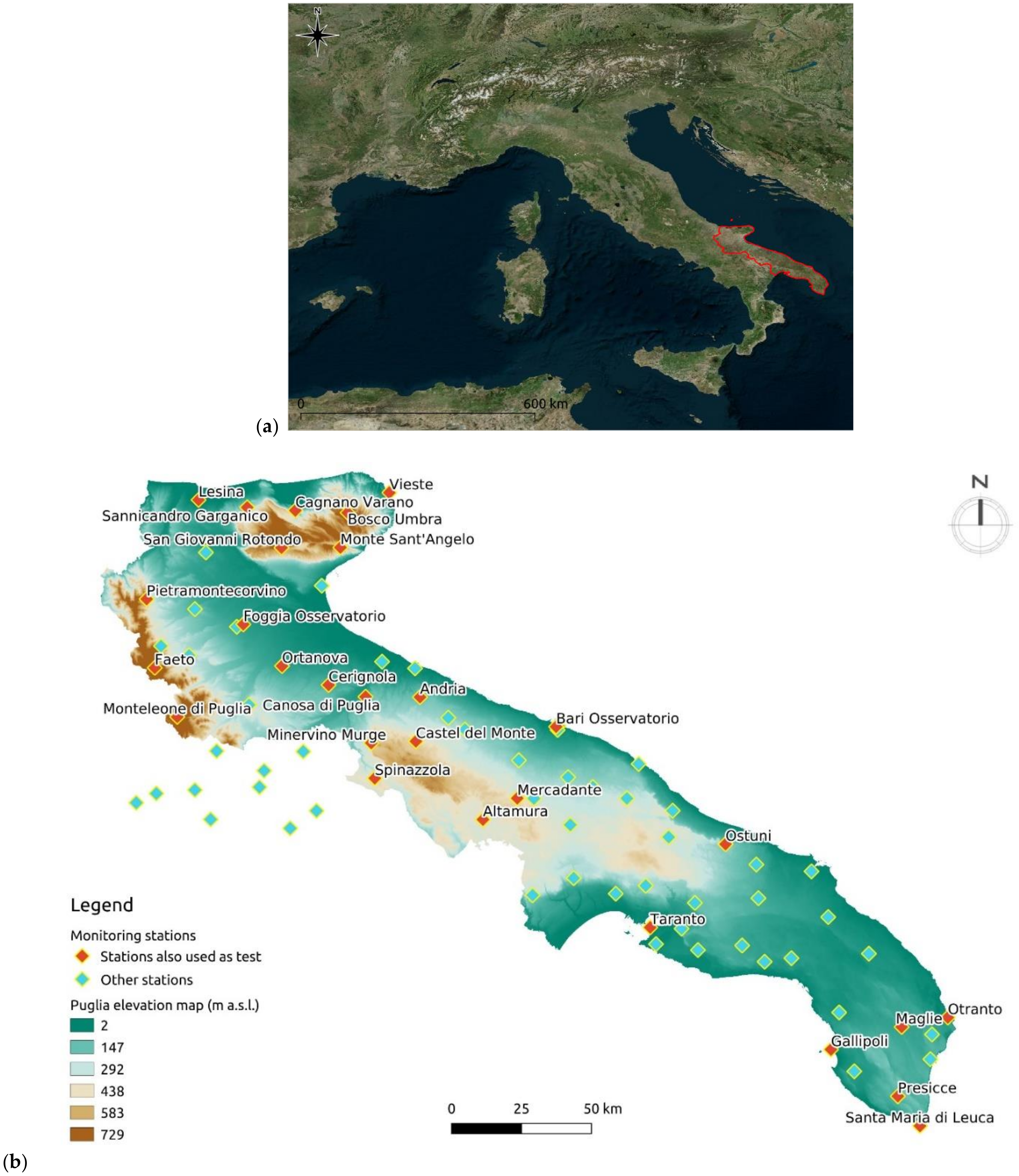
The present study is focused on the area of the Puglia Region, the easternmost part of the Italian peninsula, which covers around 19,500 km2.
The Puglia region is located within latitudes 39°47′ N and 42°13′ N, longitudes 14°50′ E and 18°31′ E, with altitudes ranging from sea level to 1150 m (Figure 1a).
This region is dominated by the Mediterranean macroclimate, more or less significantly modified by the influence of several geographic sectors and the complex surface morphology. Due to its particular geographic position and the accentuated territorial discontinuity, the Puglia region has highly diversified microclimatic conditions within both the various regional geographic districts and the Mediterranean macroclimate, from which it is dominated. The Adriatic side is markedly affected by the continental climate, and the north-western part is influenced by the mountain climate of the nearby Campania-Lucan Apennines contrasted to the south by the Ionian Sea and the central Mediterranean.
In the Puglia region, a Regional Agrometeorological Service and Civil Protection (a governmental structure of the Italian Republic in charge of the coordination of activities on prediction, prevention, management and overcoming of disasters, calamities, human and natural) provide data from a total number of stations of more than 150 acquiring information simultaneously. In Figure 1b, there is the map of the stations.
2.2. Used Dataset and Monitoring Networks
The data utilised for this study come from the sensors of the monitoring stations of the weather stations from Civil Protection of the Puglia region and the Regional Association of Defense Consortiums of Puglia. Sensors from these monitoring stations measure rainfall, temperature, relative and absolute humidity, wind direction, leaf wetness, atmospheric pressure, global radiation and wind speed.
Based on available data, the datasets used include ten years (2003–2013) of monthly cumulative rainfall of n. 81 stations and hourly measured air temperature to ground for n. 94 stations for six years (2011–2016).
The rainfall data and temperature were used to test and evaluate our algorithm. Below, we report the results for only rainfall, that is, the climate variable with the highest spatial–temporal variability and also a fundamental driver of processes related to the occurrence of natural disasters (floods and landslides) or extreme events (drought and wetness) [36]. The temperature data were also used to develop and implement the DSS in a real case, i.e., to predict values and monitor frost phenomena on a continuous spatial scale, especially those declared by farmers to request financial support from the Region.
We used a subset greater than 30% of the available data from stations to test our algorithm AIDW compared to the common IDW.
Network density is one station every 108 km2, and there is a maximum elevation difference of more than 600 m (from the highest to the lowest).
Monitoring networks are physical systems similar to graphs, in which a set of nodes (the stations) are connected using doubly oriented arcs. In the field of information theory, each station (node) can be considered a source of information where the latter is transmitted through hypothetical virtual channels (arcs) from one node to another. It is known that monitoring networks are designed with a degree of redundancy [37] to pass the known information that is measured in the node to the whole scale [38,39,40]. This scale jump occurs by superimposing a regular grid to the area of interest and estimating the values of the variable observed in the nodes in the grid points. The estimate, in general, takes place by averaging the observed values in the nodes that are placed around the points of the estimation grid. The weights’ values mainly depend on the intensity of the spatial influence that exists between the point of the grid and the nodes that surround it.
2.3. The Inverse Distance Weighted Algorithm Implementation
The Inverse Distance Weighted (IDW) method calculates the distances between the point of which to estimate value and the nodes of the network that fall within a predefined surrounding distance, implementing the assumption that things that are close to one another are more similar than those that are farther apart [41].
These distances are added together, and each is standardised for the sum. Each node is pre-multiplied by the weight obtained at the value observed, and the estimate of the unknown node is the result of the average weighted values.
The weights assigned to the interpolating points are the inverse of their distance from the interpolation point. Consequently, the close points are made up to have more weights (so more impact) than distant points and vice versa.
With IDW methodology, the point to estimate is called k, and the nodes of the network that surround k are designated with the index i:
with i = 1, …, N, it is the vector of the inverted distances in the N nodes of the network;
with i = 1, …, N, it is the vector of the observations in the N nodes of the network;
This is the sum of the inverted distances useful for weight standardization;
This is the estimate of the value of the variable of interest in the unknown point.
2.4. The Augmented Inverse Distance Weighted Algorithm Implemented
The IDW method is improvable because the distance between the unknown point and the observation nodes of the network, although important as an indicator, may not be the only factor to consider. Therefore, to obtain a more reliable estimate, other elements could be considered in defining the weights attributed to the observed values. It is clear that these new elements to be considered are not absolute but depend strictly on the variable that is intended to interpolate. In the specific case in which the climatological variables of interest are the rainfall and temperature, an element that must undoubtedly be taken into consideration is the difference in elevation between the point to be estimated and the respective nodes of the network to provide more relevant results for mountainous regions where topographic impacts on precipitation are essential [42].
The methodology AIDW has been implemented considering the monitoring network with the station representing the nodes using topographic data [43].
The matrices and weights will follow the formulas given below according to the hierarchical order of application:
Calculation of distances:
with
Calculation of heights:
with
Calculation of weights:
Weighted average:
with i = 1, …, N as the vector of the N nodes of the network.
The values in the nodes will be multiplied by the Wik weights and average (according to Equation (10)), obtaining the estimate at the unknown point. The methodology is susceptible to improvement through the introduction of other descriptors (topographic and not) such as distance from the sea (for precipitation and humidity) or indicators of correlation between stations (in the case of significant morphologic variation), which requires further in-depth activities as they are site-specific.
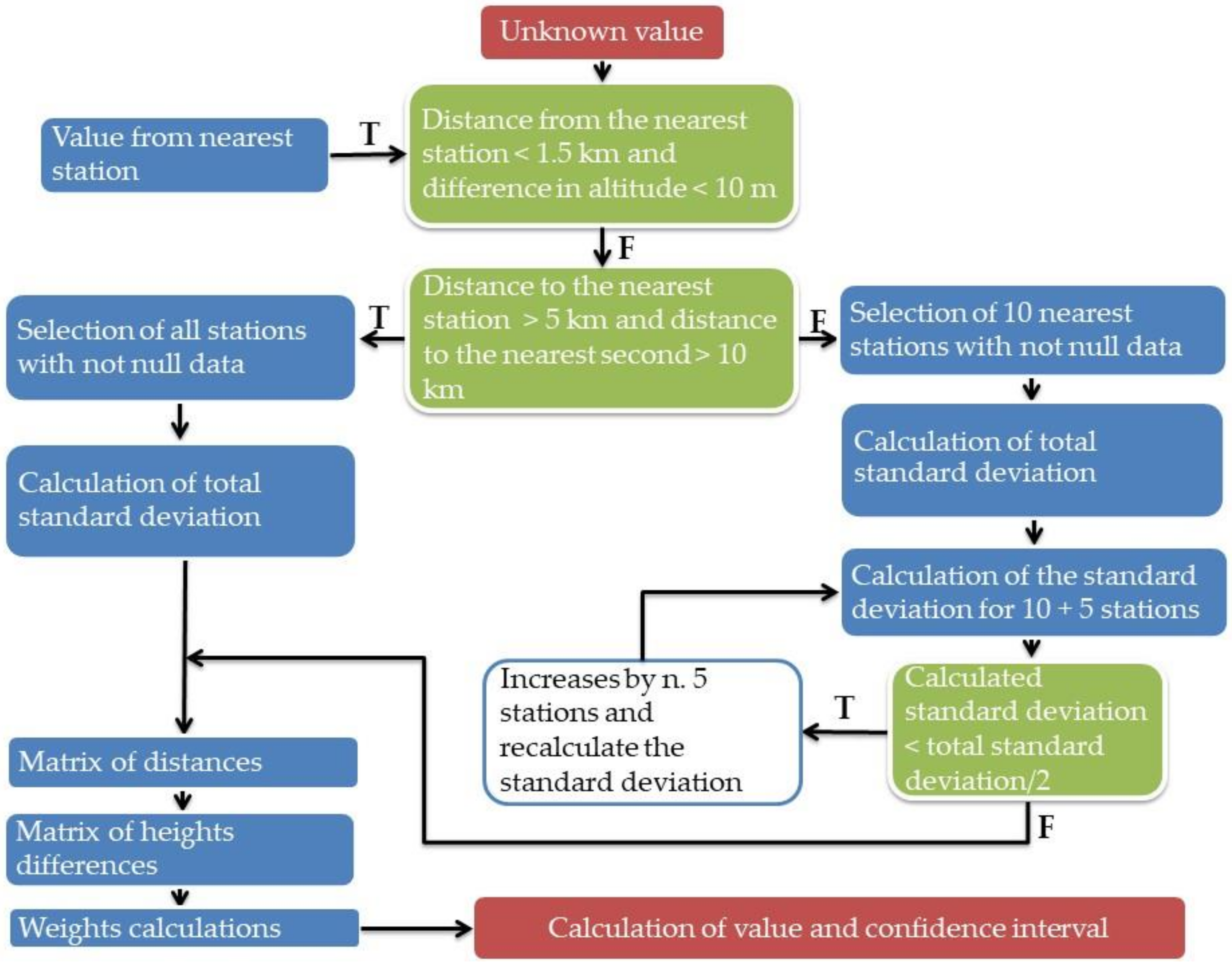
The AIDW algorithm has been implemented based on a decision tree diagram implemented through an if-then-else nested statement in the open-source scripting language python [44]. Python is a high-level language, object-oriented, suitable among other uses to develop scripting because it is portable, rich in libraries, and so can be integrated with other languages with a consistent number of python bindings [45] that are packages and extensions tools for programming and manipulating the Geospatial Data Abstraction Library (GDAL) [46]. So, we used the following Free and Open-Source libraries. The main python modules implemented are osgeo, ogr, gdal, pyproj, Proj, transform, math, datetime, itemgetter, etc.
This DSS is based on the geographical characteristics of stations, their mutual position, the availability of data of neighbouring stations and the standard deviation of the values measured by both neighbouring and total stations.
In Figure 2, we report the rules implemented in the decision algorithm to be replicated in other contexts and according to one’s needs. All the rules implemented have been subject to validation and contextualized to the geomorphological and meteorological peculiarities of the Puglia region territory.
To represent the decision framework, different colours have been arbitrarily chosen to identify the various phases of procedural programming represented by blocks of source code (called sub-routines or procedures in computer language). Each is characterised by the fact that performs a specific function within the whole program. Typically, such sub-routines are identifiable as decision-making statements that guide a program to make decisions based on specified criteria.
Coloured red blocks represent input and output data. The critical aspects that will have to be considered are mainly those related to the distribution of weather stations in the territory. In fact, in some areas, it is not possible to provide reliable data, while in certain conditions it is suggested to provide output data in an interval calculated by an n. 3 standard deviation value of the considered stations to provide as output a confidence interval [47].
In this case, the first station closest to the point to be calculated is more than 5 km away and the second more than 10 km (these values are empirical and came from our tests in very extreme situations), so we suggest multiplying with a coefficient up to 4 [47]. It is known that the confidence interval represents the range of values in which it is likely to find the predicted value accurately. It corresponds to 68% of possibility if it varies by the value of the standard deviation, by 95% if it varies by the value of the standard deviation multiplied by 1.96, and up to 99% if the coefficient with which to multiply the standard deviation is 2.58 [48].
2.5. Cross-Validation
A comparative analysis between the results obtained by applying our augmented algorithm and the classical inverse distance weighted is shown and discussed.
To validate the predictive model and verify the reliability of the results, Cross-Validation (CV) or the so-called “leave-one-out” technique, which is a statistical resampling method, has been used [49].
Cross-validation involves eliminating each observation, estimating the value at its site from the remaining observations and comparing the predicted value with the measured value. This procedure is a rapid, inexpensive approach for comparing predicted and measured values and is closely related to the statistical method of jack-knife estimation [50].
Proceeding in this way, we selected 28 stations in slightly different microclimatic conditions relative to the stations that surround them (based on our knowledge of the area) and stations that do not have many other stations nearby or surrounding and applied the CV technique. For each station considered to validate the method, the corresponding series was removed from the dataset; the precipitation and temperature values were calculated at the station’s location. Then, the calculation of the performance indicators, as described below, was performed and we compared the expected results (calculated with our AIDW) with those measured by the station whose series, as we said before, was removed from the dataset to apply these tests.
To evaluate the performance of the spatial interpolation results made with AIDW, three different statistical scores, among the most commonly used accuracy measures, have been calculated for both spatial interpolation methods (IDW and AIDW), and then the results were compared.
Performance evaluation criteria used in the current study have been calculated using the average of the absolute values of errors between the measured and calculated data (MAE) [51,52], the Root-Mean-Square Error (RMSE) [51,53] and the average of the ratio between the measured and calculated data and measured value (MRE) [54], computed as follows.
The Mean Absolute Error (MAE) is the average of all absolute errors. The formula is:
where:
n = the number of the measures;
|xi − x| = the absolute errors between measured and predicted values.
The Root-Mean-Square Error (RMSE) is a common way to measure the error in predicting quantitative data, the formula is:
where:
xi are the observed values;
x are predicted values;
n the number of observations.
Mean Relative Error (MRE) is also computed starting from Relative Error (RE) for each data set. The formula is:
where n is the number of datasets and with:
Each of these statistical error indicators emphasizes different features of the results and provides specific information on the true reliability of the method. As for indicators of the spatial interpolation scheme performance and the estimated values’ accuracy, each of them presents some inherent drawbacks associated with its definition.
MAE and RMSE are measures of accuracy of the interpolation, which should be as small as possible for more accurate interpolation [55]. MAE is conceptually simpler and more accessible to interpret than RMSE. Being only the average vertical or horizontal distance between each point, it represents the absolute difference between the predicted and measured values. The RMSE is mainly related to the standard deviation of forecast errors and therefore has a solid statistical sense. The squared function is very sensitive to extreme values as it puts much weight on significant errors [56] and errors smaller than one [57]. Compared to the previous MAE, RMSE involves squaring the differences so that a few significant differences will increase the RMSE to a greater degree than the MAE [58]. The RMSE value measures the absolute error in which deviations are squared to prevent positive and negative values from cancelling each other out. Therefore, with this measure, the errors of greater value are amplified, a characteristic that can eliminate the methods that have the most significant errors.
MRE is also used to measure the accuracy (closeness of the measurements to a specific value), which is the ratio of the absolute error of a measurement to the measurement being taken; in other words, this type of error is relative to the size of the item being measured.
3. Results and Discussion
Below, we report the results of the monthly cumulative rainfall, known as the climate variable with the highest spatial–temporal variability [36], as the hourly values of the temperatures showed minor variations. Therefore, the discussion would not be interesting for the reader.
In the following part, we report the results from different test stations located throughout the territory (Figure 1b) selected based on different altitudes, knowledge of different microclimatic conditions due to different factors such as the presence of nearby karst gorges, steep slopes or strong wind, or because of secluded positions in the sense that other stations do not surround them. We report for each of them the coordinates, the elevation, and the calculated values, proceeding with the CV validation technique of the performance indicators for MAE, RMSE and MRE for both AIDW and IDW. Since these are indicators of accuracy, the logic is “the smaller, the better”; i.e., the best is the one that takes the smallest value. The difference is not great but still significant given that the sample is large. In addition, we report in columns a, b, c and d some test results obtained comparing the indicators in a way that is understandable to the reader, i.e., 1 if true, 0 if false (Table 1).
From a descriptive point of view, the MAE minimum values were calculated for the Bari Osservatorio station and the maximum for Bosco Umbra. For RMSE, the minimum was found in Ostuni and the maximum was always in Boso Umbra. Finally, for MRE, the minimum for AIDW was in Cagnano Varano and IDW was in Foggia Osservatorio, while the highest was in Bari Osservatorio.
The value calculated for AIDW is less than that calculated for IDW for n. 23 out of 28 cases for the EAW, 22 out of 28 for RMSE and 20 out of 28 for MRE.
This implies that for the test stations considered for the data series, i.e., accumulated monthly rainfall in 10 years, considering only one of the performance indicators, the results obtained for AIDW are better performing than those obtained on IDW from 71% to 82%. For 16 stations, i.e., 57% of the test stations, all three indicators are aligned, i.e., the value calculated for AIDW is always lower than that calculated for IDW. In all these cases, the AIDW is better than the simple IDW.
These stations vary between those at low altitudes and close to the sea, for example, Taranto, Santa Maria di Leuca, to the one with a high altitude and a considerable distance from the sea, that is Faeto. It is reported that most of the stations where there are no correspondences between the three performance indicators are located at high altitudes where the climatic conditions are very variable and where mountain ranges could also act as a barrier to precipitation carried by air currents. These stations are, for example, Bosco Umbra, Monte Sant’Angelo, Monteleone di Puglia (in the latter two, IDW seems to perform better than AIDW). In these last two stations, we must recognize that the introduction of the weight of the altitude in the calculation of the spatialized value negatively affects the prediction (this may be due to the strong wind recorded). As can be seen from the map in Figure 1b, the Faeto station is positioned near two other stations, making the output data much more reliable. Otherwise, the Monteleone di Puglia and Monte Sant’Angelo stations not only are not near other stations, but they are not even surrounded by other stations and, being also in situations of different microclimate, the introduction of the altitude is a factor that could increase the error because another variable influences the precipitation, that is the wind. Therefore, if a station is not surrounded by others, further investigations should be made before introducing the quota, perhaps using the method based on these three performance indicators, while if we do not fall into these situations, the AIDW algorithm is more performant and this must be taken into consideration also given that it is possible to implement it with open-source software, it is low cost and can be integrated into other complex DSS systems.
Finally, regarding the distances from the sea, the rainfall values do not seem to be influenced by this parameter which could undoubtedly be helpful in the case of spatialisation of the absolute and relative humidity values.
Comparing our AIDW with previous studies, we can consider it a good compromise between deterministic (IDW) and geostatistical (OK, KED, COK, EBK) methods. On the one hand, deterministic methods are based on “the postulation that the rainfall value at an unsampled point can be estimated as the distance-weighted average of the rainfall values at sampling points” [32]. On the other hand, geostatistical interpolation algorithms involve the use of variables associated with the measured points in the prediction of the values in unknown points [32]. Our implemented algorithm combines both approaches considering different parameters, “in our case elevation”, associated with available data to improve missing data prediction. Usually, previous studies demonstrated better accuracy of more sophisticated geostatistical methods, e.g., KED and COK [32,59], than deterministic ones in terms of applicability to rainfall estimation.
However, some authors [59] observed similar good performance between IDW and OK for precipitation estimation. Furthermore, the great advantages of our AIDW are its simplicity and speed in returning information (a few seconds of computational time). The information is provided on demand in a point-like manner.
Therefore, it is not necessary to have large servers for storing information as high-resolution distribution maps are not produced. This is translated in an easy, rapid and low-cost customizable tool.
The effect of implementing algorithms adding complementary information on rainfall data should depend on the level of correlation among variables and the richness of pluviometric stations. Usually, high estimation accuracy is obtained when a very dense station network is available [60]. However, the accuracy of estimation is also highly correlated to the study area, time scale and precipitation. Therefore, there is no method appropriate for all circumstances and sometimes the efficiency of more sophisticated algorithms is not greater than that of simple ones [60,61,62,63].
4. Conclusions
Geospatial interpolation, implemented through the introduction of other factors into the weight calculation and through low-cost and open-source scripting languages, whose paradigm is based on an Augmented Inverse Distance Weighted algorithm, allow deriving more accurate pluviometric and thermometric values for unknown points. This is very useful for evaluating frosts, drought events and consequently better managing crop damage and related compensation. For example, this application proved to be very useful for identifying claims that were not truthful and for which compensation for crop loss was not provided. The algorithm created represents a solution implemented in on-demand mode as it can respond to different requests that must make use of different input data: if there is a request for compensation due to drought or frost, it can occur if the request is appropriate and follows up on refunds. This is the main application it carries out to date.
The methodology implemented also allows us to understand the geographical areas that need a greater concentration of monitoring stations, increasing network density. These considerations can be extrapolated from the calculated values of performance indicators, which prove to be very useful for understanding the added value of spatialized data, making us understand, at the same time, which factors most influence the recorded values and which must be considered for a more precise spatialisation.
This methodology could also be adopted, for its simplicity of implementation in any context, from applications for local administrators to applications in the search field, for example, the integration for a more accurate calculation of various climatic and bioclimatic indices and graphs [64,65,66,67] or to improve local weather reports.
All these indexes can provide more detailed and more functional information for adequate agricultural management, giving simple information of immediate use for the application and execution of various administrative procedures related to the management of agro-ecosystems.
Moreover, following simple precautions, they can be used in the different regional territories of reference following the project’s specific needs that arise from the bodies responsible for the local government.
With regard to the data available, the processing of the information provided by the various monitoring stations can also provide an overview of the current climate change trends and allow the adoption of appropriate strategies for reducing impacts in the agricultural sector. It is known that any changes in the frequency and intensity of extreme events can significantly impact society, agriculture, industry, and a functional ecosystem. An evaluation of historical data, whose historical series can also be reconstructed with this proposed methodology where they were not available, is essential for providing indications on trends and better planning of management policies considering site-specific conditions. From the analysis of a robust dataset indicating the current climatic trend, it is potentially possible to reduce the risks deriving from phenomena, such as intense precipitation (floods and landslides) and other risk factors such as population density and policies related to land utilisation.
Author Contributions
Conceptualization, C.M. and C.C.; methodology, C.M. and C.C.; software, C.M.; validation, C.M. and C.C.; formal analysis, C.M. and C.C.; investigation, C.M. and C.C.; resources, C.M. and V.F.U.; data curation, C.M. and C.C.; writing—original draft preparation, C.M. and C.C.; writing—review and editing, C.M. and C.C.; visualization, C.M. and C.C.; supervision, C.M.; project administration, C.M. and V.F.U.; funding acquisition, V.F.U. All authors have read and agreed to the published version of the manuscript.
Funding
This study was financed by Assocodipuglia, which associates the Defense Consortia of Intensive Production of the five Puglia region provinces legally established and recognized under the National and Regional Laws.
Institutional Review Board Statement
Not applicable.
Informed Consent Statement
Not applicable.
Data Availability Statement
Not applicable.
Acknowledgments
The authors thank Emanuele Barca for the precious support and collaboration in writing the AIDW algorithm and Charmaigne Pumihic for her essential help in correcting the first draft.
Conflicts of Interest
The authors declare no conflict of interest.
References
- Alfaro-Saiz, E.; García-González, M.E.; del Río, S.; Penas, Á.; Rodríguez, A.; Alonso-Redondo, R. Incorporating bioclimatic and biogeographic data in the construction of species distribution models in order to prioritize searches for new populations of threatened flora. Plant Biosyst. 2015, 149, 827–837. [Google Scholar] [CrossRef] [Green Version]
- Shul’gin, A.M. Bioclimatology as a Scientific Discipline and Its Current Objectives. Sov. Geogr. 1960, 1, 67–74. [Google Scholar] [CrossRef]
- Pignatti, S. Ecologia Vegetale; UTET: Turin, Italy, 1995; ISBN 8802046700. [Google Scholar]
- Stocker, T.F.; Qin, D.; Plattner, G.K.; Tignor, M.M.B.; Allen, S.K.; Boschung, J.; Nauels, A.; Xia, Y.; Bex, V.; Midgley, P.M. Climate Change 2013—The Physical Science Basis: Working Group I Contribution to the Fifth Assessment Report of the Intergovernmental Panel on Climate Change; Cambridge University Press: Cambridge, UK, 2014; Volume 9781107057999, pp. 1–1535. [Google Scholar] [CrossRef] [Green Version]
- Sectors Affected. Available online: https://ec.europa.eu/clima/eu-action/adaptation-climate-change/how-will-we-be-affected/sectors-affected_en (accessed on 24 December 2021).
- UNDESA World Social Report 2020|DISD. Available online: https://www.un.org/development/desa/dspd/world-social-report/2020-2.html (accessed on 24 December 2021).
- Zhai, Z.; Martínez, J.F.; Beltran, V.; Martínez, N.L. Decision support systems for agriculture 4.0: Survey and challenges. Comput. Electron. Agric. 2020, 170, 105256. [Google Scholar] [CrossRef]
- Massarelli, C.; Ancona, V.; Galeone, C.; Uricchio, V.F. Methodology for the implementation of monitoring plans with different spatial and temporal scales of plant protection products residues in water bodies based on site-specific environmental pressures assessments. Hum. Ecol. Risk Assess. Int. J. 2019, 26, 1341–1358. [Google Scholar] [CrossRef]
- Viggiano, M.; Busetto, L.; Cimini, D.; Di Paola, F.; Geraldi, E.; Ranghetti, L.; Ricciardelli, E.; Romano, F. A new spatial modeling and interpolation approach for high-resolution temperature maps combining reanalysis data and ground measurements. Agric. For. Meteorol. 2019, 276–277, 107590. [Google Scholar] [CrossRef]
- Wackernagel, H. Multivariate Geostatistics. Earth-Sci. Rev. 1999, 48, 132–133. [Google Scholar] [CrossRef]
- Hudson, G.; Wackernagel, H. Mapping temperature using kriging with external drift: Theory and an example from scotland. Int. J. Climatol. 1994, 14, 77–91. [Google Scholar] [CrossRef]
- Hungerford, R.D.; Nemani, R.R.; Running, S.W.; Coughlan, J.C. MTCLIM: A Mountain Microclimate Simulation Model; Res. Pap. INT-RP-414; US Department of Agriculture, Forest Service, Intermountain Research Station: Ogden, UT, USA, 1989; Volume 414, p. 52. [Google Scholar] [CrossRef]
- Thornton, P.E.; Running, S.W.; White, M.A. Generating surfaces of daily meteorological variables over large regions of complex terrain. J. Hydrol. 1997, 190, 214–251. [Google Scholar] [CrossRef] [Green Version]
- Vicente-Serrano, S.M.; Saz-Sánchez, M.A.; Cuadrat, J.M. Comparative analysis of interpolation methods in the middle Ebro Valley (Spain): Application to annual precipitation and temperature. Clim. Res. 2003, 24, 161–180. [Google Scholar] [CrossRef] [Green Version]
- Luo, Z.; Johnson, D.R. Spatial-Temporal Analysis of Temperature Using Smoothing Spline ANOVA. J. Clim. 1997, 11, 18–28. [Google Scholar] [CrossRef]
- Jiang, H.; Schörgendorfer, A.; Hwang, Y.; Amemiya, Y. A pratical approach to spatio-temporal analysis. Stat. Sin. 2015, 25, 369–384. [Google Scholar] [CrossRef] [Green Version]
- Sahu, S.K.; Mardia, K.V. Recent trends in modeling spatio-temporal data. In Proceedings of the Meeting of the Italian Statistical Society on Statistics and the Environment, Messina, Italy, 21–23 September 2005; pp. 69–83. [Google Scholar]
- Im, H.K.; Rathouz, P.J.; Frederick, J.E. Space–time modeling of 20 years of daily air temperature in the Chicago metropolitan region. Environmetrics 2009, 20, 494–511. [Google Scholar] [CrossRef]
- Loubier, J.C. Optimizing the Interpolation of Temperatures by GIS: A Space Analysis Approach. Mathematics 2010, 97–107. [Google Scholar] [CrossRef]
- Jian, W.; Zhili, S.; Qiang, Y.; Rui, L. Two accuracy measures of the Kriging model for structural reliability analysis. Reliab. Eng. Syst. Saf. 2017, 167, 494–505. [Google Scholar] [CrossRef]
- Kurtzman, D.; Kadmon, R. Mapping of temperature variables in Israel: Sa comparison of different interpolation methods. Clim. Res. 1999, 13, 33–43. [Google Scholar] [CrossRef] [Green Version]
- Liberoff, A.L.; Flaherty, S.; Hualde, P.; García Asorey, M.I.; Fogel, M.L.; Pascual, M.A. Assessing land use and land cover influence on surface water quality using a parametric weighted distance function. Limnologica 2019, 74, 28–37. [Google Scholar] [CrossRef]
- Pimentel, R.; Lopes, D.J.H.; Mexia, A.M.M.; Mumford, J.D. Validation of a geographic weighted regression analysis as a tool for area-wide integrated pest management programs for Ceratitis capitata Wiedemann (Diptera: Tephritidae) on Terceira Island, Azores. Int. J. Pest Manag. 2016, 63, 172–184. [Google Scholar] [CrossRef]
- Firozjaei, M.K.; Nematollahi, O.; Mijani, N.; Shorabeh, S.N.; Firozjaei, H.K.; Toomanian, A. An integrated GIS-based Ordered Weighted Averaging analysis for solar energy evaluation in Iran: Current conditions and future planning. Renew. Energy 2019, 136, 1130–1146. [Google Scholar] [CrossRef]
- Singh, V.; Xiaosheng, Q. Data assimilation for constructing long-term gridded daily rainfall time series over Southeast Asia. Clim. Dyn. 2019, 53, 3289–3313. [Google Scholar] [CrossRef]
- Radi, N.F.A.; Zakaria, R.; Azman, M.A.Z. Estimation of missing rainfall data using spatial interpolation and imputation methods. AIP Conf. Proc. 2015, 1643, 42–48. [Google Scholar] [CrossRef] [Green Version]
- Suhaila, J.; Deni, S.M.; Jemain, A.A. Revised spatial weighting methods for estimation of missing rainfall data. Asia-Pac. J. Atmos. Sci. 2008, 44, 93–104. [Google Scholar]
- CLIMPAG|DATA and MAPS|LocClim: Local Climate Estimator. Available online: https://www.fao.org/nr/climpag/pub/en0201_en.asp (accessed on 25 November 2021).
- Dobesch, H.; Dumolard, P.; Dyras, I. Spatial Interpolation for Climate Data: The Use of Gis in Climatology and Meteorology; John Wiley & Sons: Hoboken, NJ, USA, 2007; p. 284. [Google Scholar]
- Liu, Y.; Chen, Z.; Hu, B.D.; Jin, J.K.; Wu, Z. A non-uniform spatiotemporal kriging interpolation algorithm for landslide displacement data. Bull. Eng. Geol. Environ. 2019, 78, 4153–4166. [Google Scholar] [CrossRef]
- Wu, C.Y.; Mossa, J.; Mao, L.; Almulla, M. Comparison of different spatial interpolation methods for historical hydrographic data of the lowermost Mississippi River. Ann. GIS 2019, 25, 133–151. [Google Scholar] [CrossRef]
- Pellicone, G.; Caloiero, T.; Modica, G.; Guagliardi, I. Application of several spatial interpolation techniques to monthly rainfall data in the Calabria region (southern Italy). Int. J. Climatol. 2018, 38, 3651–3666. [Google Scholar] [CrossRef]
- Tobler, W.R. A Computer Movie Simulating Urban Growth in the Detroit Region. Econ. Geogr. 1970, 46, 234. [Google Scholar] [CrossRef]
- Chi Siamo|Agrometeopuglia—ARIF PUGLIA. Available online: http://www.agrometeopuglia.it/chi-siamo (accessed on 24 December 2021).
- FAO and the 2030 Agenda for Sustainable Development|Sustainable Development Goals|Food and Agriculture Organization of the United Nations. Available online: https://www.fao.org/sustainable-development-goals/overview/fao-and-the-2030-agenda-for-sustainable-development/en/ (accessed on 27 December 2021).
- Lyra, A.; Tavares, P.; Chou, S.C.; Sueiro, G.; Dereczynski, C.; Sondermann, M.; Silva, A.; Marengo, J.; Giarolla, A. Climate change projections over three metropolitan regions in Southeast Brazil using the non-hydrostatic Eta regional climate model at 5-km resolution. Theor. Appl. Climatol. 2017, 132, 663–682. [Google Scholar] [CrossRef]
- Wang, C.; Zhao, L.; Sun, W.; Xue, J.; Xie, Y. Identifying redundant monitoring stations in an air quality monitoring network. Atmos. Environ. 2018, 190, 256–268. [Google Scholar] [CrossRef]
- Kanevski, M.; Volpi, M.; Copa, L.; Kanevski, M.; Volpi, M.; Copa, L. Environmental Monitoring Networks Optimization Using Advanced Active Learning Algorithms. EGUGA 2010, 12, 2915. [Google Scholar]
- Chen, K.; Ni, M.; Cai, M.; Wang, J.; Huang, D.; Chen, H.; Wang, X.; Liu, M. Optimization of a Coastal Environmental Monitoring Network Based on the Kriging Method: A Case Study of Quanzhou Bay, China. Biomed Res. Int. 2016, 2016, 1–12. [Google Scholar] [CrossRef] [PubMed]
- Araki, S.; Iwahashi, K.; Shimadera, H.; Yamamoto, K.; Kondo, A. Optimization of air monitoring networks using chemical transport model and search algorithm. Atmos. Environ. 2015, 122, 22–30. [Google Scholar] [CrossRef] [Green Version]
- How Inverse Distance Weighted Interpolation Works—ArcGIS Pro|Documentation. Available online: https://pro.arcgis.com/en/pro-app/latest/help/analysis/geostatistical-analyst/how-inverse-distance-weighted-interpolation-works.htm (accessed on 27 December 2021).
- Masih, I.; Maskey, S.; Uhlenbrook, S.; Smakhtin, V. Assessing the Impact of Areal Precipitation Input on Streamflow Simulations Using the SWAT Model1. JAWRA J. Am. Water Resour. Assoc. 2011, 47, 179–195. [Google Scholar] [CrossRef]
- Puglia Region—Regional Planning Service Office Digital Terrain Model of Puglia Region. Available online: http://webapps.sit.puglia.it/freewebapps/DTM/index.html (accessed on 28 November 2021).
- Welcome to Python.org. Available online: https://www.python.org/ (accessed on 27 December 2021).
- Welcome to the Python GDAL/OGR Cookbook!—Python GDAL/OGR Cookbook 1.0 Documentation. Available online: http://pcjericks.github.io/py-gdalogr-cookbook/index.html# (accessed on 3 June 2021).
- GDAL—GDAL Documentation. Available online: https://gdal.org/index.html (accessed on 3 June 2021).
- Kanevski, M.; Maignan, M. Analysis and Modelling of Spatial Environmental Data; EPFL Press: Lausanne, Switzerland, 2004; p. 288. [Google Scholar]
- Field, A. Discovering Statistics Using IBM SPSS Statistics (Electronic Version); SAGE Publications, Inc.: New York, NY, USA, 2017; ISBN 9781526445766. [Google Scholar]
- Allen, D.M. The Relationship between Variable Selection and Data Agumentation and a Method for Prediction. Technometrics 1974, 16, 125–127. [Google Scholar] [CrossRef]
- Efron, B. The Jackknife, the Bootstrap and Other Resampling Plans; Society for Industrial and Applied Mathematics: Philadelphia, PA, USA, 1982. [Google Scholar]
- Willmott, C.J.; Matsuura, K. Advantages of the mean absolute error (MAE) over the root mean square error (RMSE) in assessing average model performance. Clim. Res. 2005, 30, 79–82. [Google Scholar] [CrossRef]
- Fürnkranz, J.; Chan, P.K.; Craw, S.; Sammut, C.; Uther, W.; Ratnaparkhi, A.; Jin, X.; Han, J.; Yang, Y.; Morik, K.; et al. Mean Absolute Error. Encycl. Mach. Learn. 2011, 652. [Google Scholar] [CrossRef]
- Chai, T.; Draxler, R.R. Root mean square error (RMSE) or mean absolute error (MAE)?—Arguments against avoiding RMSE in the literature. Geosci. Model Dev. 2014, 7, 1247–1250. [Google Scholar] [CrossRef] [Green Version]
- Li, W.E.I.; Chen, J.I.E.; Li, L.U.; Chen, H.U.A.; Liu, B.; Xu, C.Y.; Li, X. Evaluation and bias correction of S2S precipitation for hydrological extremes. J. Hydrometeorol. 2019, 20, 1887–1906. [Google Scholar] [CrossRef]
- Johnston, K.; Ver Hoef, J.M.; Krivoruchko, K.; Lucas, N. Using ArcGIS geostatistical analyst. Analysis 2001, 300, 300. [Google Scholar]
- Hernandez-Stefanoni, J.L.; Ponce-Hernandez, R. Mapping the spatial variability of plant diversity in a tropical forest: Comparison of spatial interpolation methods. Environ. Monit. Assess. 2006, 117, 307–334. [Google Scholar] [CrossRef]
- Montgomery, D.C.; Johnson, L.A.; Gardiner, J.S. Forecasting and Time Series Analysis, 2nd ed.; McGraw-Hill: New York, NY, USA, 1990; ISBN 9780070428584. [Google Scholar]
- Pontius, R.G.; Thontteh, O.; Chen, H. Components of information for multiple resolution comparison between maps that share a real variable. Environ. Ecol. Stat. 2007, 15, 111–142. [Google Scholar] [CrossRef]
- Berndt, C.; Haberlandt, U. Spatial interpolation of climate variables in Northern Germany—Influence of temporal resolution and network density. J. Hydrol. Reg. Stud. 2018, 15, 184–202. [Google Scholar] [CrossRef]
- Hu, Q.; Li, Z.; Wang, L.; Huang, Y.; Wang, Y.; Li, L. Rainfall Spatial Estimations: A Review from Spatial Interpolation to Multi-Source Data Merging. Water 2019, 11, 579. [Google Scholar] [CrossRef] [Green Version]
- Lloyd, C.D. Assessing the effect of integrating elevation data into the estimation of monthly precipitation in Great Britain. J. Hydrol. 2005, 308, 128–150. [Google Scholar] [CrossRef]
- Moral, F.J. Comparison of different geostatistical approaches to map climate variables: Application to precipitation. Int. J. Climatol. 2010, 30, 620–631. [Google Scholar] [CrossRef]
- Dirks, K.N.; Hay, J.E.; Stow, C.D.; Harris, D. High-resolution studies of rainfall on Norfolk Island: Part II: Interpolation of rainfall data. J. Hydrol. 1998, 208, 187–193. [Google Scholar] [CrossRef]
- Rivas-Martinez, S. Clasificacìon Bioclimàtica de la tierra. Folia Bot. Madritensis 1996, 16, 1–32. [Google Scholar]
- Walter, H. Klimadiagramm Weltatlas; [s.n.]: [S.l.]; ConchBooks: Harxheim, Germany, 1980. [Google Scholar]
- Thornthwaite, C. The Water Balance; Drexel Institute of Technology Laboratory of Climatology: Centerton, NJ, USA, 1955. [Google Scholar]
- Mckee, T.B.; Doesken, N.J.; Kleist, J. The relationship of drought frequency and duration to time scales. In Proceedings of the 8th Conference on Applied Climatology, Anaheim, CA, USA, 17–22 January 1993; pp. 17–22. [Google Scholar]
Figure 1.
(a) The borders of the Puglia region; (b) used monitoring stations for this study. We also reported the stations from which values were used as tests. The label refers to the Italian name of the station, which we will use in the paper. Note: the stations without underlying Puglia elevation map are located in another region, but the data were available for this study.

Figure 2.
The decision framework for the AIDW algorithm implemented in the Decision Support System for agricultural purposes. Legend. Colour red: input and output data. Colour green: box for choosing alternatives (T = True, F = False). Colour blue: operation to be performed. Colour white: operation to be performed until the condition is verified.


Table 1.
Summary table of the results obtained through the cross-validation technique and the application of the performance indicators to the predicted values with both AIDW and IDW.
Table 1.
Summary table of the results obtained through the cross-validation technique and the application of the performance indicators to the predicted values with both AIDW and IDW.
| Station Name | X (WGS84 UTM33N) | Y (WGS84 UTM33N) | Elevation (m) | MAE AIDW | MAE IDW | RMSE AIDW | RMSE IDW | MRE AIDW | MRE IDW | a | b | c | d |
|---|---|---|---|---|---|---|---|---|---|---|---|---|---|
| Altamura | 630998.1 | 4520285.1 | 482 | 1.285 | 1.651 | 2.603 | 2.742 | 0.798 | 0.915 | 1 | 1 | 1 | 1 |
| Andria | 608484.7 | 4564039.9 | 162 | 1.302 | 1.532 | 2.58 | 2.713 | 1.538 | 1.764 | 1 | 1 | 1 | 1 |
| Bari Osservatorio | 657148.7 | 4553462.8 | 34 | 0.853 | 0.895 | 2.687 | 2.727 | 2.51 | 2.53 | 1 | 1 | 1 | 1 |
| Bosco Umbra | 582616.4 | 4629940.4 | 798 | 40.472 | 49.962 | 57.167 | 69.01 | 0.544 | 0.604 | 1 | 1 | 1 | 1 |
| Cagnano Varano | 563907.1 | 4630768.9 | 181 | 18.298 | 22.088 | 27.638 | 32.821 | 0.354 | 0.393 | 1 | 1 | 1 | 1 |
| Canosa di Puglia | 589011.6 | 4564170.4 | 154 | 9.59 | 10.559 | 13.968 | 14.665 | 0.434 | 0.542 | 1 | 1 | 1 | 1 |
| Castel del Monte | 607008.9 | 4548253.3 | 543 | 10.891 | 12.258 | 15.604 | 17.532 | 0.359 | 0.3487 | 1 | 1 | 0 | 0 |
| Cerignola | 575810.8 | 4568397.3 | 134 | 9.524 | 9.799 | 14.136 | 14.134 | 0.361 | 0.415 | 1 | 0 | 1 | 0 |
| Faeto | 513658.1 | 4574523.6 | 776 | 18.198 | 21.136 | 26.913 | 30.886 | 0.469 | 0.482 | 1 | 1 | 1 | 1 |
| Foggia Osservatorio | 545323.2 | 4590048.3 | 82 | 6.592 | 18.213 | 9.92 | 22.736 | 0.994 | 0.242 | 1 | 1 | 0 | 0 |
| Gallipoli | 755424.5 | 4438104.3 | 31 | 14.421 | 18.285 | 21.706 | 27.312 | 1.001 | 1.269 | 1 | 1 | 1 | 1 |
| Lesina | 529318.2 | 4634539.7 | 13 | 15.609 | 20.296 | 22.272 | 27.745 | 0.58 | 0.815 | 1 | 1 | 1 | 1 |
| Maglie | 780678.2 | 4446165.2 | 102 | 16.387 | 15.266 | 25.21 | 23.875 | 0.483 | 0.445 | 0 | 0 | 0 | 0 |
| Mercadante | 643260.5 | 4527900.7 | 393 | 9.788 | 14.002 | 14.517 | 20.750 | 0.407 | 0.533 | 1 | 1 | 1 | 1 |
| Minervino Murge | 591064.4 | 4547652 | 454 | 14.455 | 15.201 | 21.912 | 23.975 | 0.5238 | 0.456 | 1 | 1 | 0 | 0 |
| Monte Sant’Angelo | 580020.1 | 4617529.6 | 817 | 31.072 | 23.303 | 44.037 | 37.777 | 0.888 | 0.494 | 0 | 0 | 0 | 0 |
| Monteleone di Puglia | 521705.7 | 4556971.7 | 844 | 17.303 | 16.103 | 24.054 | 22.647 | 0.387 | 0.361 | 0 | 0 | 0 | 0 |
| Ortanova | 559151.7 | 4575168.9 | 80 | 10.031 | 11.373 | 14.655 | 15.769 | 0.489 | 0.674 | 1 | 1 | 1 | 1 |
| Ostuni | 717709.9 | 4511508.1 | 234 | 1.465 | 1.915 | 2.529 | 2.687 | 0.38 | 0.41 | 1 | 1 | 1 | 1 |
| Otranto | 797186.8 | 4449554.4 | 29 | 19.485 | 20.424 | 32.041 | 33.768 | 0.697 | 0.747 | 1 | 1 | 1 | 1 |
| Pietramontecorvino | 510754.6 | 4599088.4 | 225 | 21.552 | 20.281 | 32.161 | 30.353 | 0.375 | 0.46 | 0 | 0 | 1 | 0 |
| Presicce | 779316.6 | 4421387.7 | 105 | 17.573 | 20.337 | 29.074 | 34.574 | 0.719 | 0.71 | 1 | 1 | 0 | 0 |
| San Giovanni Rotondo | 558967 | 4617451.4 | 572 | 18.855 | 22.163 | 27.969 | 32.652 | 0.426 | 0.423 | 1 | 1 | 0 | 0 |
| Sannicandro Garganico | 546701.7 | 4631844.5 | 236 | 20.781 | 23.665 | 32.693 | 37.232 | 0.415 | 0.466 | 1 | 1 | 1 | 1 |
| Santa Maria di Leuca | 787239 | 4410792.4 | 26 | 18.084 | 19.071 | 27.272 | 28.871 | 0.886 | 1.07 | 1 | 1 | 1 | 1 |
| Spinazzola | 592315 | 4535068.4 | 458 | 13.928 | 12.775 | 19.764 | 17.861 | 0.492 | 0.524 | 0 | 0 | 1 | 0 |
| Taranto | 690795.7 | 4481728 | 27 | 9.584 | 15.934 | 14.442 | 21.804 | 0.549 | 0.984 | 1 | 1 | 1 | 1 |
| Vieste | 597511.9 | 4637115.5 | 53 | 15.835 | 16.576 | 22.974 | 23.581 | 0.701 | 0.76 | 1 | 1 | 1 | 1 |
| TOT | 23 | 22 | 20 | 17 |
Legend. Results of the comparison tests between the performance indicator for AIDW and IDW according to the rule if AIDW < IDW is true then 1, otherwise 0, for: (a) MAE. (b) RMSE. (c) MRE. (d) Result of the comparison test between of the agreement of the three indicators, if all three are 1 then the value is 1, otherwise 0; TOT is the sum of the calculated values present in the column above.
Publisher’s Note: MDPI stays neutral with regard to jurisdictional claims in published maps and institutional affiliations. |
© 2022 by the authors. Licensee MDPI, Basel, Switzerland. This article is an open access article distributed under the terms and conditions of the Creative Commons Attribution (CC BY) license (https://creativecommons.org/licenses/by/4.0/).
Share and Cite
MDPI and ACS Style
Massarelli, C.; Campanale, C.; Uricchio, V.F. Custom Methodology to Improve Geospatial Interpolation at Regional Scale with Open-Source Software. Knowledge 2022, 2, 88-102. https://0-doi-org.brum.beds.ac.uk/10.3390/knowledge2010005
AMA Style
Massarelli C, Campanale C, Uricchio VF. Custom Methodology to Improve Geospatial Interpolation at Regional Scale with Open-Source Software. Knowledge. 2022; 2(1):88-102. https://0-doi-org.brum.beds.ac.uk/10.3390/knowledge2010005
Chicago/Turabian StyleMassarelli, Carmine, Claudia Campanale, and Vito Felice Uricchio. 2022. "Custom Methodology to Improve Geospatial Interpolation at Regional Scale with Open-Source Software" Knowledge 2, no. 1: 88-102. https://0-doi-org.brum.beds.ac.uk/10.3390/knowledge2010005