
The Benefit of Horizontal Photovoltaic Panels in Reducing Wind Loads on a Membrane Roofing System on a Flat Roof

1
National Institute of Technology (KOSEN), Akita College, Akita 011-8511, Japan
2
Tohoku Electric Power Network Corporation, Sendai 980-8551, Japan
3
S.B. Sheet Waterproof Systems Co., Ltd., Kanuma 322-0014, Japan
*
Author to whom correspondence should be addressed.
Wind 2021, 1(1), 44-62; https://0-doi-org.brum.beds.ac.uk/10.3390/wind1010003
Submission received: 8 September 2021
/
Revised: 29 October 2021
/
Accepted: 30 October 2021
/
Published: 9 November 2021
Abstract
:The present paper proposes a measure for improving the wind-resistant performance of photovoltaic systems and mechanically attached single-ply membrane roofing systems installed on flat roofs by combining them together. Mechanically attached single-ply membrane roofing systems are often used in Japan. These roofing systems are often damaged by strong winds, because they are very sensitive to wind action. Recently, photovoltaic (PV) systems placed on flat roofs have become popular. They are also often damaged by strong winds directed onto the underside, which cause large wind forces onto the PV panels. For improving the wind resistance of these systems, we proposed to install PV panels horizontally with gaps between them. Such an installation may decrease the wind forces on the PV panels due to the pressure equalization effect as well as on the waterproofing membrane due to the shielding effect of the PV panels. This paper discusses the validity of such an idea. The pressure on the bottom surface of a PV panel, called the “layer pressure” here, was evaluated by a numerical simulation based on the unsteady Bernoulli equation. In the simulation, the time history of the external pressure coefficients, measured at many points on the roof in a wind tunnel, was employed. It was found that the wind forces, both on the PV panels and on the roofing system, were significantly reduced. The reduction was large near the roof’s corner, where large suction pressures were induced in oblique winds. Thus, the proposed method improved the wind resistance of both systems significantly.
1. Introduction
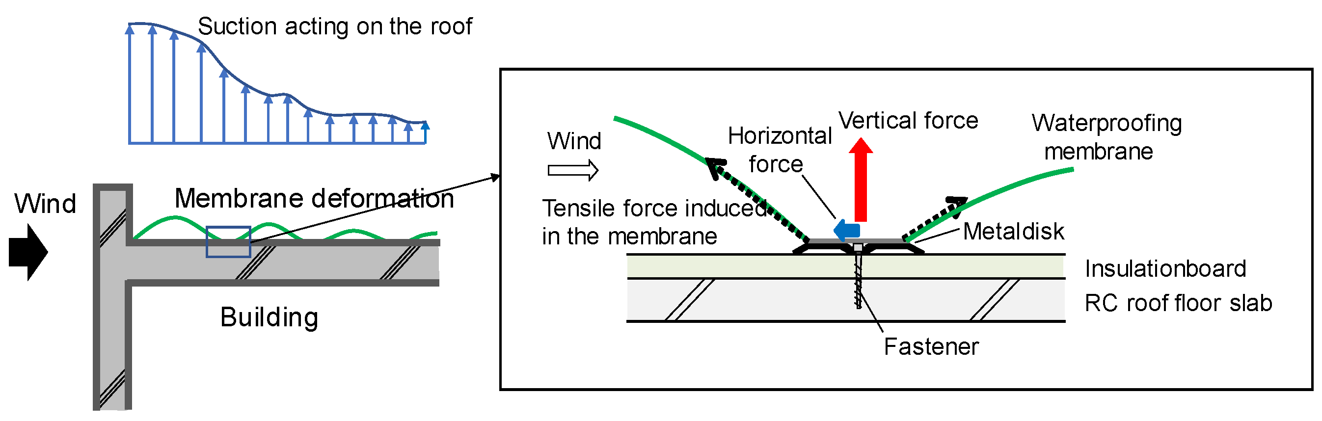
Mechanically attached single-ply membrane roofing systems are widely used for flat roofs in Japan because of their high workability, low installation cost, and consideration of environmental conservation; the amount of adhesive used for this system is much lower than that of conventional adhesion methods. Figure 1 shows a typical construction method used on roofs of reinforced concrete buildings. In this system, a waterproofing membrane is fixed to a roof’s substrate with many fasteners, which are generally arranged in a square lattice-like form with a spacing of 0.45–1.0 m. Note that this construction method is somewhat different from that generally used in Europe and North America, where membranes are anchored to a roof’s substrate by a series of fasteners arranged along the seams of the membranes (see Baskaran and Borujerdi [1], for example). In any case, roofing systems are generally sensitive to wind actions. Consequently, they are often damaged by strong winds [2]. Billowing of membranes due to the fact of high suction pressures may cause tears in the membrane or pull-out of the fasteners [3]. Therefore, for the safety design of this roofing system, it is important to evaluate the wind resistance of the roofing system appropriately. Cook [4] experimentally investigated the wind-induced dynamic behavior of single-ply membrane roofing systems using a full-scale specimen. Test methods for evaluating the wind resistance of mechanically attached waterproofing systems have been investigated by many researchers, e.g., Gerhardt and Kramer [5,6], Baskaran and Chen [7], and Baskaran et al. [8]. In conventional test methods, including the above-mentioned ones, the specimen is subjected to spatially uniform pressure, which may be static or dynamic. This type of loading generates only vertical forces on the fasteners. Miyauchi et al. [9] carried out a field measurement of wind pressures and wind-induced responses (membrane deformations and loads on fasteners) of a mechanically attached single-ply membrane roofing system installed on a full-scale flat-roofed test building without parapets during a typhoon. They found that fasteners located near the windward corner were subjected to horizontal forces as large as vertical ones. Then, they carried out a pressure test and a wind tunnel test using a full-scale roofing assembly [10]. In the pressure test, uniform pressure was applied to the bottom surface of the membrane. Accordingly, no horizontal force was generated on the fasteners. In the wind tunnel test, on the other hand, the test model was immersed in a turbulent flow. In this case, the wind pressures (suctions) on the membrane varied in the windward direction. As a result, the membrane deflection also varied in this direction (see Figure 2). There was larger deformation-induced tension in the membrane, resulting in larger vertical and horizontal forces at the fixing point. The resultant horizontal force at the fixing point was provided by the difference between the horizontal components of the membrane tensions in the windward and leeward directions as schematically illustrated in Figure 2. This feature was investigated by Sugiyama et al. [11] and Uematsu et al. [12] both experimentally and numerically. It is thought that the horizontal force affects the wind-resistant performance of the roofing systems significantly, because the horizontal force generates a moment at the fixing point of the fastener that may reduce the fastener’s pull-out resistance significantly.
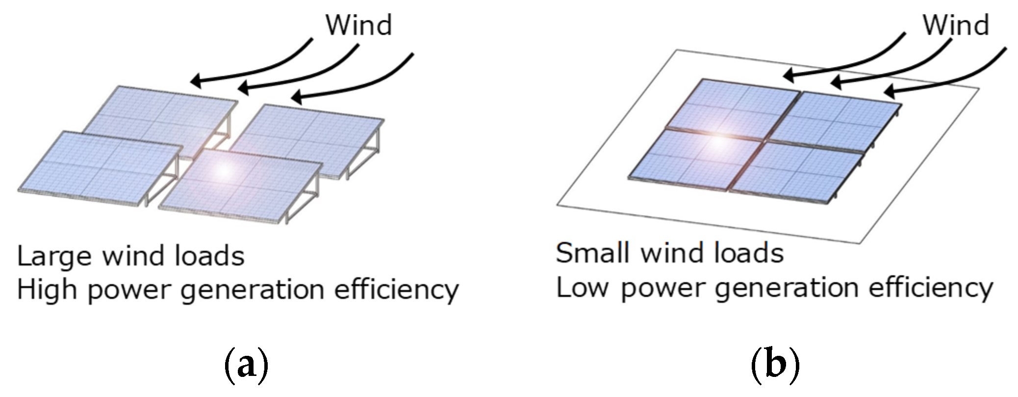
For improving the wind resistance of a roofing system, it seems effective to reduce the vertical and horizontal forces acting on the fasteners. For this purpose, we propose to use photovoltaic (PV) panels as a wind-load reduction device for a roofing system. Wind loads on PV panels placed on flat roofs have been investigated by many researchers [13,14,15]. PV panels are usually installed at a tilt angle of 20–30° with respect to the roof’s surface. In this case, the PV panels are subjected to large wind forces in a wind directed onto the underside. On the other hand, when PV panels are placed horizontally, the wind forces become small (Figure 3), although the power generation efficiency decreases.
In the present paper, we propose to install PV panels horizontally, parallel to a flat roof. Furthermore, small gaps are provided between them. Figure 4 schematically illustrates the wind forces acting on a roofing system (a) when PV panels are not installed and (b) when PV panels are installed. Without PV panels, large suction pressures act on the membrane directly. With PV panels, on the other hand, the membrane is subjected to “layer pressure”, i.e., pressure of the space between the roof’s surface and the bottom surface of the PV panel. The wind force acting on the PV panel may decrease significantly due to the effect of “pressure equalization” caused by the gaps. At the same time, the external pressure acting on the membrane may also decrease.
For evaluating the wind loads on the PV panels and roofing system appropriately, it is necessary to estimate the layer pressure accurately. It is quite difficult to measure the layer pressure experimentally in a wind tunnel, because we cannot make a wind tunnel model of a PV system with such a small geometric scale as 1/100; the gap between the roof’s surface and the bottom surface of a PV panel is generally as small as approximately 10 cm. Therefore, a numerical simulation based on the unsteady Bernoulli equation was applied to this problem. Similar approaches have been applied to wind-load estimation of air-permeable double-layer roof systems, loose-laid roof-insulation systems, and roofing tiles [16,17,18,19,20].
It should be noted that the present paper is an extended version of our previous papers [21,22]. The previous papers outlined the simulation method and focused only on the wind pressures on PV panels and waterproofing membranes. In the present paper, the simulation method and the simulated results are described in detail. Furthermore, the wind-induced responses of the roofing system (i.e., the membrane deformation and the wind forces acting on the fasteners) are also investigated.
2. Investigated Building and Roofing System
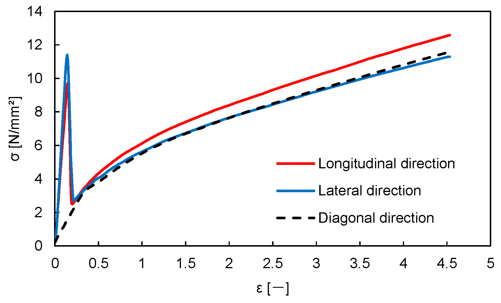
The main subject of the present study was a mechanically attached single-ply membrane roofing system installed on the flat roof of a low-rise building with parapets such as a residential house. Note that this is a case study. The breadth (B), depth (D), and height (H) of the building were 8, 8, and 10 m, respectively. The height (hp) and thickness (tp) of the parapets were both 0.15 m (see Figure 5). The waterproofing membrane was a polyvinyl chloride (PVC) resin sheet of approximately 1.5 mm in thickness, reinforced by glass fibers of 560 dTex with a density of 3.6 fibers per 10 mm in both the longitudinal and transverse directions. The mass per unit area was 2.044 kg/m2. Figure 6 shows the stress (σ)–strain (ε) relationship for the longitudinal, lateral, and diagonal directions obtained from a tensile test with No. 2 dumbbell-type specimens 10 mm wide. Note that we also tested with No. 3 dumbbell-type specimens 5 mm wide to obtain the material properties of the membrane. Regarding the specimens for the longitudinal and lateral directions, the tensile strength rapidly changed at ε 15%. This phenomenon was due to the fracture of glass fibers. After the glass fibers broke, the σ–ε curves were almost the same as that for the diagonal (45°) direction, which was further found to be almost the same as that for the unreinforced membrane. The membrane was anchored to the structural substrate using PVC-coated circular steel disks 65 mm in diameter and 1.2 mm in thickness and fasteners (i.e., screws). The disks were arranged in a square lattice-like form with a spacing of 0.6 m, to which the membrane was attached with a solvent.
3. Wind Tunnel Experiment of Wind Pressure Distributions
3.1. Experimental Method
The objective of the present experiment was to determine the most critical condition (i.e., wind direction and roof zone) providing the largest suction pressure on the waterproofing membrane. The time history of wind pressure coefficients at many locations under such a condition were used for simulating the layer pressures in Section 4, the results of which were used for analyzing the dynamic response of the waterproofing membrane in Section 5.
The wind tunnel model was made with a geometric scale of λL = 1/100. The PV system was not modeled. Figure 7 shows the arrangement of pressure taps. The diameter of the pressure taps was 0.5 mm. It is well-known that very large suction pressures are generated near the windward corner in oblique winds [23,24,25,26]. Therefore, the pressure taps were densely arranged in the corner and edge zones. The wind direction (θ), defined as shown in Figure 7, was changed from 0 to 45° at an increment of 5°.
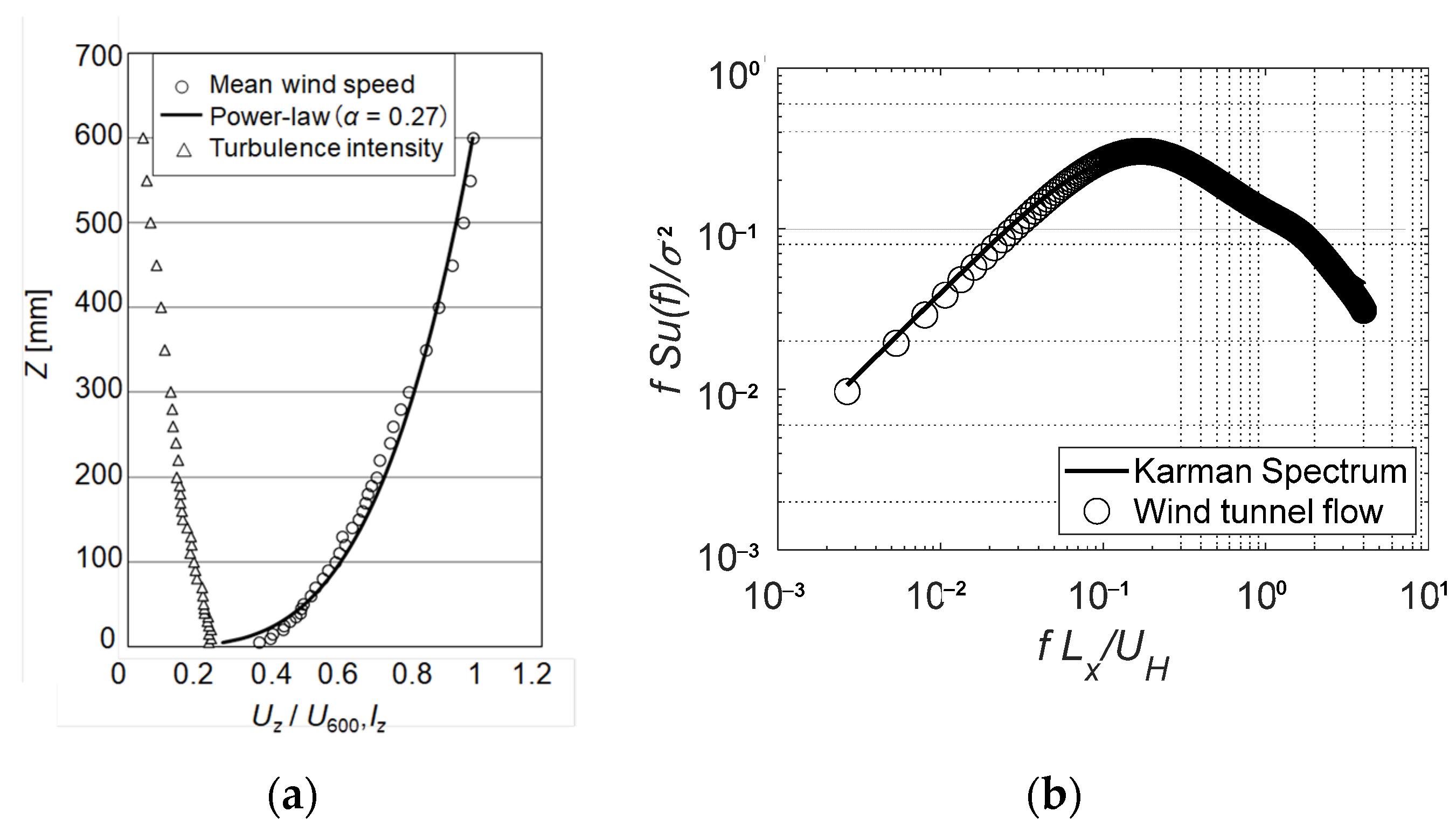
The wind tunnel experiment was conducted in an Eiffel-type wind tunnel, at Tohoku University, that had a working section 1.4 m wide, 1.0 m high, and 6.5 m long. The wind tunnel flow was a turbulent boundary layer generated on the floor using a standard spire-roughness technique. Figure 8a shows the profiles of the mean wind speed (UZ), normalized by a value at a reference height of Z = 600 mm, and the turbulence intensity, IZ. The power-law exponent α of the mean wind speed profile was approximately 0.27. The turbulence intensity, IZ, at Z = 100 mm was approximately 0.16. Figure 8b shows the normalized spectral energy density distribution at Z = 100 mm, which corresponded well to the Karman-type spectrum with an integral length scale, Lx, of approximately 0.2 m. The present study did not focus on a specific building in a specific area. However, these values were compared to the specified values in the AIJ Recommendations for Loads on Buildings [27] for Terrain Category III (suburban exposure). According to the Recommendations, these values are specified as α = 0.20, IZ = 0.24, and Lx = 57.7 m (at full scale). The value of α of the wind tunnel flow was larger than the specified value, while the values of IZ and Lx of the wind tunnel flow were smaller than the specified values. Such discrepancies can be accepted, because the main purpose of this study was to discuss the application of PV panels for the improvement of the wind resistance of mechanically attached single-ply membrane roofing systems and not to evaluate wind loads for designing a PV system and a roofing system.
The design wind speed, UH at Z = H, was determined based on the AIJ Recommendations for Loads on Buildings [27], assuming that the “Basic wind speed” U0 was 35 m/s and the terrain category was III. Indeed, UH was calculated as 27.8 m/s. The value of UH was set to 8 m/s in the wind tunnel experiment. The Reynolds number defined by was approximately 5.3 × 10⁴, where represents the coefficient of the kinematic viscosity of air. The blockage ratio (Br) of the model, with respect to the wind tunnel working section area, was approximately 0.8%. The Reynolds number and the blockage ratio satisfied the experimental criteria recommended in Wind Tunnel Testing for Buildings and Other Structures [28]; that is, Re was larger than 1.1 × 10⁴, and Br was smaller than 5%. The velocity and time scales, λV and λT, of the wind tunnel experiment were 1/3.48 and 1/28.8, respectively. Wind pressures at all pressure taps were sampled simultaneously at a rate of 800 Hz for a time duration of 10 min at full scale (approximately 20.8 s at model scale) using a multi-channel pressure measuring system (Wind Engineering Institute, MAPS-02). The internal diameter and length of the tubes connecting the pressure taps and the pressure transducers were 1 mm and 1 m, respectively. A low-pass filter with a cut-off frequency of 300 Hz was used to remove high-frequency noise from the signals. The measurements were repeated 10 times. The measured wind pressure was converted to a pressure coefficient (Cpe) defined in terms of the velocity pressure (qH) of the approach flow at Z = H. Ensemble averaging was applied to the results of the 10 consecutive measurements in order to obtain the statistical values of Cpe and others. The distortion of the measured wind pressures due to the tubing was compensated in the frequency domain by using the frequency response function of the measuring system.
3.2. Experimental Results
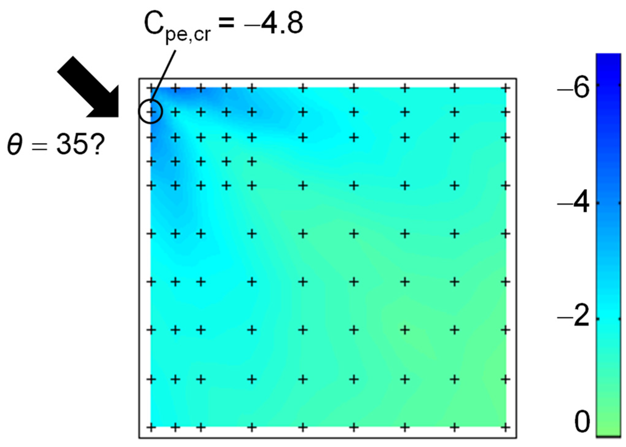
We first detected the condition (i.e., pressure tap and wind direction) generating the most critical negative peak pressure coefficient, Cpe,cr, irrespective of wind direction and tap location. We found that the value of Cpe,cr was −4.8 at a pressure tap near the windward roof corner when θ = 35°. Figure 9 shows the distribution of the minimum peak pressure coefficients in this wind direction, together with the pressure tap location represented by “+”. Note that the value at each pressure tap was the ensemble average applied to the ten results of the minimum peak pressure coefficients for a period of 10 min at full scale. It was clear that conical vortices generated large suction pressures near the windward corner as previous studies indicated [23,24,25,26]. However, the value of Cpe,cr was somewhat smaller in magnitude than those obtained in the previous studies. This may be due to the effect of the parapets [29,30,31]. Ten sets of the time history of wind pressure coefficients at θ = 35° were used for evaluating the layer pressures in Section 4 and the wind-induced responses of the roofing system in Section 5.
4. Simulation of Wind Pressures on PV Panels and Waterproofing Membrane
4.1. Method of Simulation
The simulation was made for a full-scale model in which the time history of external wind pressure coefficients obtained from the above-mentioned wind tunnel experiment were used. Thus, the layer pressures were provided as a function of time. The net wind forces on the PV panels and the wind pressures on the top surface of the waterproofing membrane were also time dependent. The outline of the simulation method for estimating the layer pressures is provided in our previous papers [21,22]. The fundamental idea is based on Amano et al. [16], Oh et al. [17], and Okada et al. [18]. In the simulation, we used the unsteady Bernoulli equation together with the time history of the external wind pressure coefficients obtained from the above-mentioned wind tunnel experiment.
The PV panel considered here was that commonly used in Japan (see Figure 10). The width, length, and depth were 977, 1257, and 21 mm, respectively. The panel was mounted in an aluminum frame, the side of which was not flat. The PV panels were installed horizontally with gaps between them on trestles 50 mm in height as shown in Figure 10a. The width of the gaps in the longitudinal direction was set to 26 mm, which made the installation of the PV panels on the frame easy. This value was tentative. The width of the gaps in the lateral direction was set to 3 mm considering the thermal expansion of the PV panels and aluminum frame. It was expected that the wind forces on the PV panels would be reduced significantly due to the pressure equalization caused by these gaps.
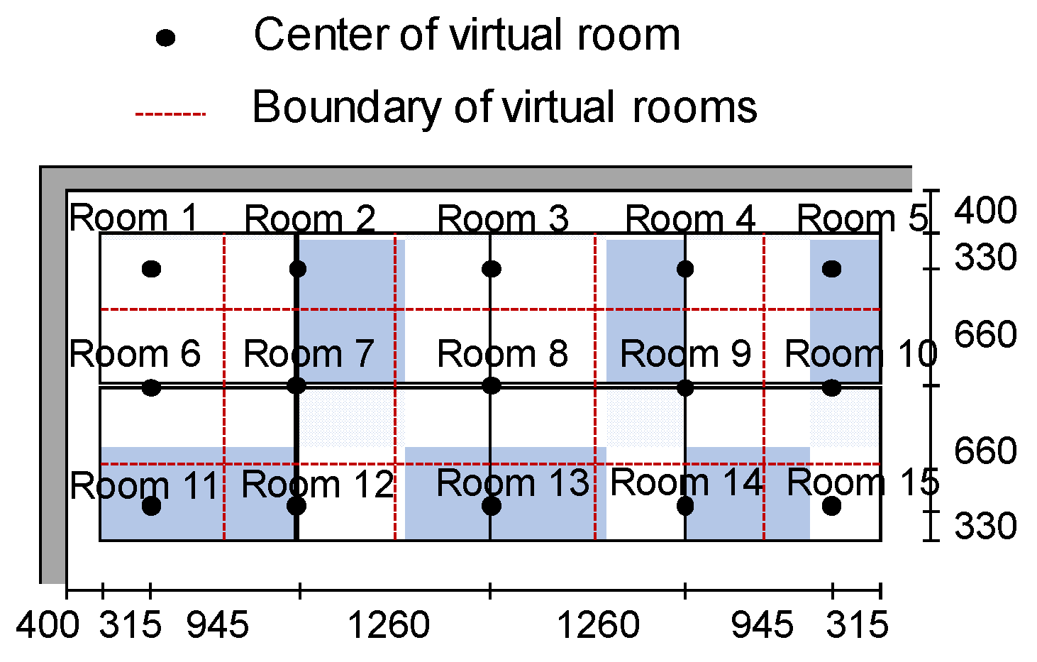
In the present analysis, eight PV panels were installed near the roof’s corner, as shown in Figure 11a, where large suction pressures are induced in oblique winds. It was expected that the effect of the PV panels on the reduction in wind forces on the roofing system would become the maximum in this zone. The panels were numbered as shown in Figure 11b. The layer pressure depends on many factors such as external pressures at the location of the gaps, gap geometry, and flow resistance of the gap and cavity flows. This is similar to the problem of building internal pressures, when the space under the PV panels is regarded as a building [16]. For evaluating the spatial variation in layer pressure, the space under the PV panels was divided into 15 sub-spaces as shown in Figure 12; the sub-spaces were called “Rooms” [20]. This was the simplest model of division that satisfied the condition that all Rooms, except for the four corner Rooms (i.e., Rooms 1, 5, 11, and 15), have gap flows in the vertical direction. The pressure in each Room (i.e., layer pressure) was time dependent but assumed spatial uniformity.
Figure 13 shows a schematic illustration of the gap and cavity flows. In the figure, P and U generally represent the room pressure and the flow speed, respectively. The subscripts i and j represent the Room number in a matrix form. For example, Room 1 is expressed as (i, j) = (1, 2) and Room 2 as (i, j) = (1, 2). The layer pressure was determined from the balance of the mass of air flowing into and out of the Room. The governing equation of the flow through the gap in the vertical direction (see Figure 13) may be represented by the unsteady Bernoulli equation as follows:
where ρ = air density; le = effective depth (slug length) of the gap; de = gap width; eUi,j = flow speed in the gap; t = time; ePi,j and Pi,j, respectively, represent the external pressure at the gap and the layer pressure of Room (i, j); CLe = pressure loss coefficient of the gap (shape resistance coefficient), depending on the gap shape; λ represents a friction coefficient, which is approximately given by the following equation assuming that the gap flow is a Hagen–Poiseuille flow [32]:
The effective depth le may be given by the following equation [33]:
where l0 and Ae represent the actual depth and area of the gap, respectively.
Similarly, the governing equation for the cavity flow under the PV panel in the x direction (see Figure 13) may be given by the following equation:
where li,j = distance from the center of a Room to that of the next Room; d = distance between the bottom surface of the PV panel and the roof; i,jUi+1,j = wind speed in the x direction from Room (i, j) to Room (i+1, j); Pi,j and Pi+1,j represent the layer pressures of Rooms (i, j) and (i+1, j), respectively; CL = shape resistance coefficient in the horizontal direction. When the boundary of a Room corresponds to the periphery of the array of PV panels, the subscript should be replaced by “e” in Equations (6) and (7). Similar equations can be obtained for the cavity flow in the y direction, not shown here to save space.
From the above equations, we can obtain the following equations for the flows in the x, y, and z directions as follows:
where eC = external pressure coefficient at the gap location; C = layer pressure coefficient; the subscript of C represents the Room location. The pressure loss coefficient CLe for the 3 mm gap between the PV panels was determined based on an experiment using a pressure loading actuator (PLA) [34] and a full-scale model of the gap. In the experiment, a full-scale model of a 3 mm gap (the length was 1000 mm) was attached to the testing wall of a chamber (the size was 900 × 830 × 200 mm), a PLA generated fluctuating pressure in the chamber using the time history of the wind pressure coefficient obtained from the wind tunnel experiment, and the pressures on both sides of the gap were measured. Then, the fluctuating pressure on the opposite side of the chamber was simulated based on the above-mentioned equation, changing the values of CLe incrementally. Comparing the simulated results with the experimental ones, we found that CLe = 1.42 provided results similar to the experimental ones. Regarding the details of this experiment, see Yambe et al. [21]. For wider gaps, we assumed that CLe = 1.0. Because the building had parapets and the installation area of the PV panels was immersed in a separated flow, it was thought that the speeds of the gap and cavity flows were relatively low. Thus, the gap and cavity flows were assumed to be laminar [17,35]. The external pressure coefficients at the gap location in Equations (9)–(11) were obtained from the above-mentioned wind tunnel experiment. Because the location of the gaps did not coincide with that of pressure taps installed on the wind tunnel model, the cubic spline function was applied to the experimental data of the wind pressure coefficients for interpolation; the value at the center of each gap was used as a representative value for the gap.
An assumption of the weak compressibility of the air and an adiabatic condition yielded a differential equation that related the internal pressure to the flow speed through the gaps as follows:
where γ is the heat capacity ratio of air; P0 is the atmospheric pressure; V0 is the volume of the Room; Qm and Um are the flow rate and flow speed at gap m, respectively; km and Am represent the discharge coefficient and area of gap m, respectively; and M is the total number of gaps. Note that the sign of Qm is positive for inflow and negative for outflow. The discharge coefficient km was determined from an experiment using a full-scale gap model and the PLA in which the flow rate and speed were measured. We found from the experiment using a full-scale model with a 3 mm gap that km = 0.55 simulated the experimental results relatively well. Regarding the details of the experiment, see Yambe et al. [21]. For wider gaps, we assumed that km = 1.0. From Equation (12), we can obtain the following equation for the layer pressure coefficient Ci,j of Room (i, j) which has a vertical gap and four adjacent Rooms:
The nonlinear simultaneous equations obtained above can be solved numerically by using a well-known Euler method of the fourth order together with the time history of the external pressures obtained from the wind tunnel experiment. The time step Δt was set to 1/8000 s based on the results of a preliminary analysis investigating the stability and accuracy of the solutions. The sampling interval of the pressure measurements in the wind tunnel experiment was approximately 0.036 s (= 1/800 s × 29) at full scale, which was much longer than Δt. Therefore, the cubic spline function was again applied to the time history of the wind pressure coefficients for interpolation.
The layer pressure in each Room was reduced to a layer pressure coefficient, Cpi, defined in terms of qH, in the same manner as Cpe. The wind force coefficient, Cf, of the PV panel may be given by:
where Cpe was obtained from the wind tunnel experiment, while Cpi was obtained from the above-mentioned numerical simulation. Similarly, the net wind pressure on the waterproofing membrane was given by the difference between pressures acting on the top and bottom surfaces of the membrane. The pressure on the top surface corresponded to the external pressure when no PV panels were placed, while it corresponded to the layer pressure when PV panels were placed. Because the pressure on the bottom surface of the membrane depended on the structural system and air tightness of the roof structure significantly, it was difficult to estimate the value generally, which may be positive or negative. Therefore, the value was assumed to be zero for simplicity. In this case, the wind force coefficient, Cf, of the membrane corresponded to the layer pressure coefficient, Cpi, or the external pressure coefficient, Cpe, whether the PV panels were installed or not.
The simulation program was made using MATLAB, which we developed by ourselves. In the simulation, we obtained ten series of the time history of Cpi and Cf for a period of 600 s at full scale. The results were used for analyzing the statistics of wind forces on the PV panels and the wind pressures on the waterproofing membrane as well as for the dynamic response analysis of the roofing system.
The above-mentioned simulation method was validated by a wind tunnel experiment [20]. In the experiment, the roof of a low-rise, flat-roofed building model was covered with a permeable panel that had small holes, constituting a kind of double-layer roof system. The layer pressures were measured at 36 locations on the roof. In the simulation, the space between the roof and the permeable plate was divided into 36 sub-spaces called “Rooms”, and the layer pressures at these Rooms were computed using the above-mentioned equations together with the time history of the external pressure coefficients at the location of the holes. It was found that the simulated results for the distributions of the mean and RMS fluctuating layer pressure coefficients were consistent with the experimental results. Then, the simulation method was employed for predicting the wind speed that caused wind-induced scatter of permeable unit flooring decks loosely laid on rooftops and balconies of high-rise buildings [20]. This simulation method was applied to the estimation of wind loads on ventilated exterior wall systems [36] as well as on PV panels installed on a hip roof [37]. In [37], almost the same simulation model and method were employed for the evaluation of layer pressures under PV panels installed on a hip roof. Comparing the simulated results with the experimental ones, the authors found that both results were consistent with each other, which implies that the simulation model and method were valid.
4.2. Results
Time history of the area-averaged wind force coefficient, Cf,panel, for each panel at θ = 35° was first computed. For computing the area-averaged wind pressure coefficient, Cpt,panel, on the top surface of a PV panel, we used the distribution of the external wind pressure coefficients obtained by applying the cubic spline function to the experimental data for interpolation. Similarly, we computed the area-averaged wind pressure coefficient, Cpb,panel, on the bottom surface of the PV panel using the layer pressure coefficients for the Rooms existing under the PV panel. The area-averaged wind force coefficient, Cf,panel, was provided by the difference between Cpt,panel and Cpb,panel. Note that the sign for Cf,panel was the same as that for Cpt,panel. We found from the results that the minimum peak value, , of Cf,panel was −1.2, which occurred on Panel 5 (regarding the panel location, see Figure 11b). This value was the ensemble average of ten results for obtained under the same condition. The positive (downward) and negative (upward) wind force coefficients of PV panels installed on flat roofs are specified in JIS C 8955 [38] as a function of the tilt angle β of PV panels. The negative value for panels with β = 0° installed near the roof corner was specified as −0.6. It should be noted that the wind force coefficient specified in the standard is defined by the minimum peak area-averaged wind force coefficient divided by a gust effect factor that depends on the terrain category and the mean roof height (H). Therefore, the present result corresponding to the minimum peak wind force coefficient should be compared with the product of the specified value and a gust effect factor. The gust effect factor for a building with H = 10 m located in an area of Terrain Category III is specified as 2.5. Therefore, the peak wind force coefficient was calculated as −0.6 × 2.5 = −1.5. This value was larger in magnitude than the minimum peak area-averaged wind force coefficient, , obtained in this study, i.e., −1.2. This result implies that the gaps between the PV panels could reduce wind loads on the PV panels due to the effect of pressure equalization.
Figure 14 shows the minimum peak external pressure coefficient, , on the roof without PV panels and the minimum peak layer pressure coefficients, , for each Room when θ = 35°. The waterproofing membrane was subjected to the external pressures, represented by the circles in the figure, when PV panels were not installed. On the other hand, the membrane was subjected to the layer pressures, represented by the squares in the figure, when PV panels were installed. It was found from this figure that the absolute value of was generally smaller than that of . Particularly, large difference could be seen near the roof corner. It can be concluded that installing PV panels horizontally with small gaps between them reduces the magnitude of suction pressures on the waterproofing membrane significantly.
5. Finite Element Analysis of the Wind-Induced Behavior of the Roofing System
5.1. Analytical Model and Procedure
For investigating the wind-induced dynamic behavior of the roofing system, we developed a 3D finite element model, using the commercial software Abaqus/CAE, in which the geometric nonlinearity of the membrane was considered. We obtained the time history of the responses of the roofing system (membrane deformations, etc.) for a period of 600 s at full scale.
The analysis was conducted on a 2.4 by 2.4 m square area located at the windward corner (see Figure 15). Most of this area was covered with PV panels. A preliminary analysis indicated that the response of the membrane in this area hardly changed, even if the analyzed area was extended. The membrane was modeled by a composite material consisting of a fiberglass layer and two PVC layers (i.e., sandwich structure) as shown in Figure 16. Because it is difficult to model glass–fiber mesh as it is, it was modeled using an anisotropic material 0.1 mm in thickness. On the other hand, PVC layers 0.7 and 0.8 mm in thickness were represented by a Mooney–Rivlin model, which is often used for super-elastic materials such as PVC [39,40]. The total thickness of the membrane was 1.51 mm. The mechanical properties of these layers were determined based on the results of material testing. Such a model for a waterproofing membrane was validated using an experiment with a 2.0 by 2.2 m full-scale specimen composed of the waterproofing membrane, nine disks, and a structural substrate (i.e., thick plywood plate) in our previous study [11,12]. In the experiment the specimen was attached to a chamber and subjected to fluctuating pressure that was generated by three PLAs based on the time history of the wind pressure coefficient obtained from a wind tunnel experiment. The membrane deformation and the forces acting on the fasteners were measured and compared to the results with those of the FE analysis. A good agreement between the experiment and FE analysis was observed for both the membrane deformation and the forces acting on the fasteners.
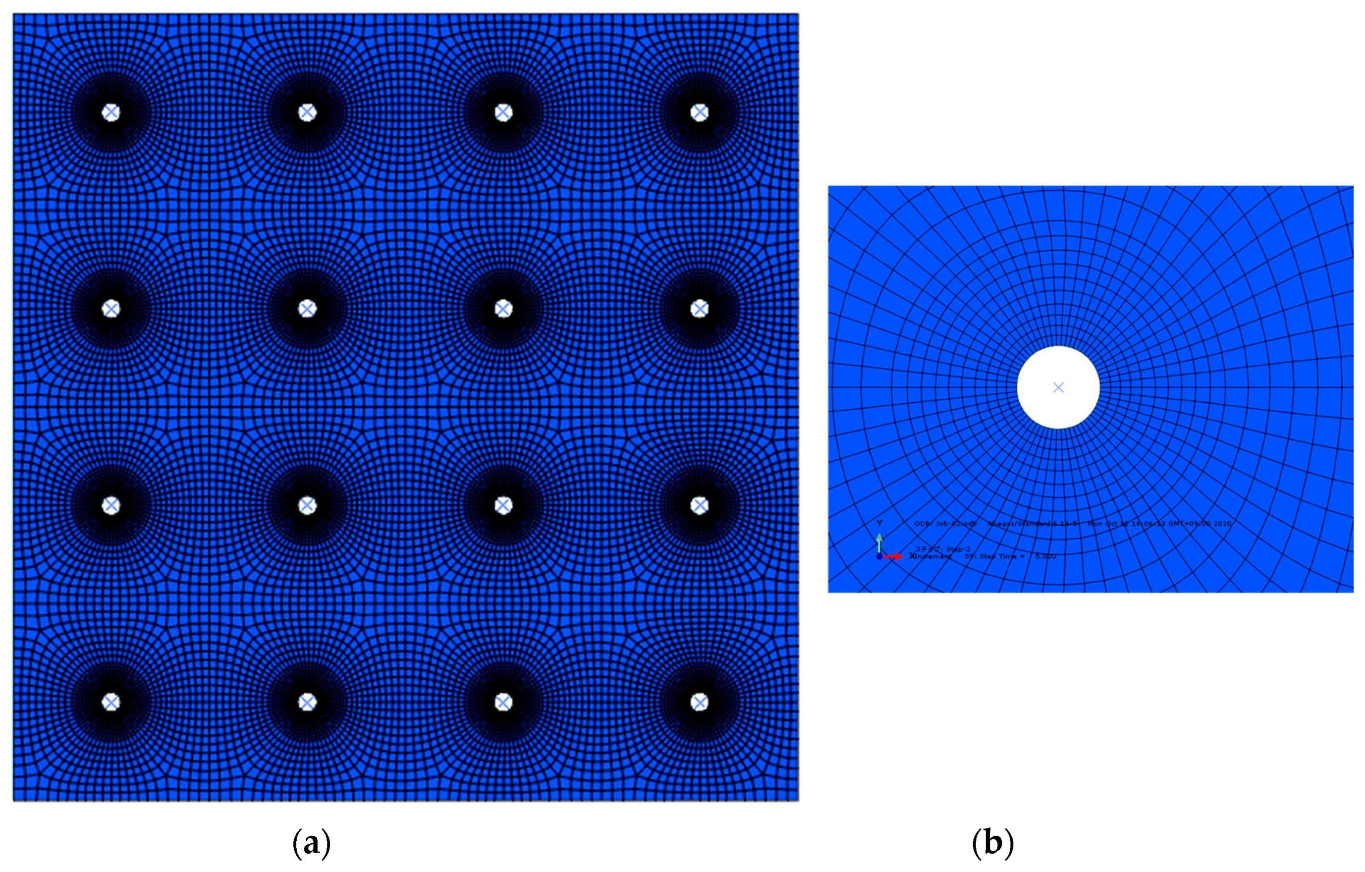
The practical values of the mechanical properties of these materials are presented in Table 1. Figure 17 shows the finite element (FE) model. Because the focus was on the wind-induced response of the membrane and the wind forces acting on the fasteners, the insulation board, fasteners, and structural substrate were not involved in the model. The areas of the membrane around the disks were divided into smaller elements. The membrane was clamped to the structural substrate along the edges. The lower surface of the membrane was fixed to circular disks 65 mm in diameter arranged in a square lattice-like form with a spacing of 0.6 m. The disks were assumed to be rigid. The membrane was represented by quadrangular shell elements. The numbers of elements and nodes were 16,384 and 17,163, respectively. The mesh division was determined based on the result of a preliminary analysis focusing on the computational accuracy and efficiency. Membrane deformation due to the suction forces may change the wind pressure distribution on the membrane (i.e., FSI effect). However, this effect was not considered in the present analysis for simplicity. In practice, the FSI effect seems small when the building has parapets. In this case, the flow separation occurred at the top of the parapet, which was minutely affected by the membrane deformation.
The Hilber–Hughes–Taylor method was employed for solving the equation of motion for the membrane. The structural damping was provided by a Rayleigh-type model, assuming that the critical damping ratios of the first and second modes were both 0.05. The wind loads at the nodes of the FE model were generated using the results of the above-mentioned wind tunnel experiment (Section 3). Because the spatial resolution of the pressure taps installed on the wind tunnel model was much coarser that that of the finite element nodes, the wind pressure coefficients at the nodes were computed by applying the cubic spline function to the experimental data for interpolation and extrapolation. In each dynamic response analysis, the time history of the wind pressure coefficients for a period of 600 s was used. The time step of computation was approximately 0.03 s. This time step was smaller than the sampling interval of wind pressure measurement in the wind tunnel experiment. Hence, we applied the cubic spline function to the time history of the wind pressure coefficients for interpolation. The computation was repeated ten times using the time history of the wind pressure coefficients obtained from the wind tunnel experiment. The statistical values of the responses were evaluated by the ensemble averages of the results of ten computations.
5.2. Results and Discussion
Figure 18 shows the results for the deflections of the membrane. The circles in the figure represent the fixing disks. Figure 18b shows the mean deformation of the membrane when the PV panels were not installed. As might be expected, the deflection became larger at the center of four fixing points, particularly along the edges. This was because these areas were subjected to large suction pressures (see Figure 9). Then, we focused on the nine points labelled from “a-1” to “c-3” in Figure 18a. In order to represent the location of the measuring points, a new coordinate system (ξ, η) was introduced as shown in Figure 18a. Figure 18c–f show the effects of the PV panels on the maximum values and the standard deviation of the deflections at nine points. It is clear that the deflections decreased significantly due to the installation of the PV panels.
The horizontal force (FH) acting on the fastener was provided by the following equation:
where Fx and Fy, respectively, represent the forces acting on the fastener in the x and y directions, which are provided by the sum of the x and y components of the forces at the nodes along the disk’s circumference. The vertical force (FV) acting on the fastener was provided by the sum of the z components of the forces at the nodes along the disk’s circumference and the force acting on the disk itself. Figure 19 shows the trajectory of the FV–FH relationship at each fixing point (see Figure 15). It was found that horizontal forces nearly equal to or larger than the vertical ones were generated on the fasteners when the PV panels were not installed. This feature corresponds well to the findings of Miyauchi et al. [9,10] and Sugiyama et al. [11]. When the PV panels were installed, the values of FV and FH were reduced significantly, except for FH at A-1.
The resultant force (F) acting on each fastener is given by:
Table 2 summarizes the maximum peak values of F at the fixing points. It was found that the maximum peak values decreased by approximately 20–40% when the PV panels were installed.
The horizontal force generated a moment on the fastener at the fixing point (roof level), which may have reduced the pull-out strength of the fastener. The present paper clearly indicates that installing PV panels horizontally over a roofing system decreases wind forces on the fastener not only in the vertical direction but also in the horizontal direction, which may improve the wind-resistant performance of a roofing system significantly. In order to evaluate the wind-resistant performance in more detail, we should investigate the failure loads and failure modes of the roofing system under practical wind loading. This is the subject of our future study.
6. Conclusions
We proposed to install PV panels horizontally with small gaps between them over mechanically attached single-ply membrane roofing systems. The pressure equalization caused by the gaps may decrease wind loads on the PV panels significantly. Furthermore, it was expected that the wind pressures on the waterproofing membrane were also reduced significantly. The reduction in wind forces on the PV system and the roofing system improved the wind-resistant performance of both systems significantly. As a result, wind-induced damage to these systems will be reduced.
In the present paper, the wind pressure distributions on a flat roof were measured in a turbulent boundary layer. The results indicated that an oblique wind caused large suction pressures on the roof near the windward corner. Then, the effects of PV panels on the wind loads and the wind-induced response of the roofing system were investigated. The pressures on the bottom surface of the PV panels, called “layer pressure” here, were numerically simulated in which we used the unsteady Bernoulli equations and the time history of the wind pressure coefficients measured at many locations on the roof in a wind tunnel. The simulation results indicated that the PV panels reduced the wind loads on the roofing system significantly. Finally, we developed a finite element model for analyzing the wind-induced responses of the roofing system. When PV panels were not installed, large suction pressures acted on the roofing system directly. On the other hand, when the PV panels were installed, the layer pressures acted on the roofing system. The results of the analysis indicated that the membrane deflections and the loads acting on the fasteners were reduced significantly by installing the PV panels.
This paper presents the results of a feasibility study investigating the application of PV panels for improvement of the wind-resistant performance of mechanically attached single-ply membrane roofing systems. In the simulation, we made many assumptions for the gap and cavity flows, such as the pressure loss coefficient (CLe), the shape resistance coefficient (CL), and the discharge coefficient (km). At present, these assumptions have not been verified yet sufficiently. Furthermore, the size of the gaps between the PV panels in the longitudinal direction was fixed to 26 mm in the present paper. This is a tentative value. Because the gap size affects the layer pressures significantly, it is necessary to investigate the effect of gap size on the layer pressures and to obtain the optimum gap size for reducing the wind loads on PV panels and the roofing system. It is also necessary to discuss the most effective arrangement of PV panels with respect to the wind-load reduction effects and the power generation efficiency.
Furthermore, it seems interesting to discuss the efficiency of the horizontal assemblage of the PV panels from an economical viewpoint. It is estimated that in Tokyo (latitude approximately 35.4° N), the power generation efficiency will decrease by approximately 10% when the tilt angle β of the PV panel is changed from the optimum value (approximately 30°) to 0°. On the other hand, the number of PV panels that can be installed in a limited area, such as the roof of a building, increases as β decreases, which may increase the total amount of the power generation output. Because the wind load on the PV panel becomes small when β = 0°, we can use a lighter frame to support the PV panels, resulting in a lower construction cost for the frame. Furthermore, the cost of a roofing system and the building structure will also decrease. As a result, wind-induced damage to the PV system and roofing system can be reduced. However, it seems difficult to assess the benefit of a horizontal installation of PV panels from an economical viewpoint, because many factors are related to this problem. Such an assessment will be important for the commercialization of the proposed system. These are the subjects of our future study.
Author Contributions
Conceptualization, Y.U.; methodology, Y.U., T.Y. and H.I.; software, T.Y.; validation, T.Y.; formal analysis, T.Y.; investigation, Y.U. and T.Y.; resources, T.W. and H.I.; data curation, T.Y. and H.I.; writing—original draft preparation, T.Y.; writing—review and editing, Y.U.; visualization, T.Y.; supervision, Y.U.; project administration, Y.U.; funding acquisition, T.W. and H.I. All authors have read and agreed to the published version of the manuscript.
Funding
This research received no external funding.
Conflicts of Interest
The authors declare no conflict of interest.
References
- Baskaran, A.; Borujerdi, J. Application of numerical models to determine wind uplift ratings of roofs. Wind. Struct. Int. J. 2001, 4, 213–226. [Google Scholar] [CrossRef]
- Japan Association for Wind Engineering, Tokyo Polytechnic University. Manual of Wind Resistant Design for Photovoltaic System; Japan Association for Wind Engineering: Tokyo, Japan, 2017. (In Japanese) [Google Scholar]
- Architectural Institute of Japan. Wind Damage in 2004 and Lessons; Architectural Institute of Japan: Tokyo, Japan, 2006. (In Japanese) [Google Scholar]
- Cook, N. Dynamic response of single-ply membrane roofing systems. J. Wind. Eng. Ind. Aerodyn. 1992, 42, 1525–1536. [Google Scholar] [CrossRef]
- Gerhardt, H.; Kramer, C. Wind induced loading cycle and fatigue testing of lightweight roofing fixations. J. Wind. Eng. Ind. Aerodyn. 1986, 23, 237–247. [Google Scholar] [CrossRef]
- Gerhardt, H.J.; Kramer, C. Wind loading and fatigue behavior of fixings and bondings of roof coverings. J. Wind. Eng. Ind. Aerodyn. 1988, 29, 109–118. [Google Scholar] [CrossRef]
- Baskaran, A.; Chen, Y. Wind load cycle development for evaluating mechanically attached single-ply roofs. J. Wind. Eng. Ind. Aerodyn. 1998, 77–78, 83–96. [Google Scholar] [CrossRef]
- Baskaran, A.; Chen, Y.; Vilaipornsawai, U. A New Dynamic Wind Load Cycle to Evaluate Mechanically Attached Flexible Membrane Roofs. J. Test. Eval. 1999, 27, 249. [Google Scholar] [CrossRef]
- Miyauchi, H.; Katou, N.; Tanaka, K. Force transfer mechanism on fastener section of mechanically anchored waterproofing membrane roofs under wind pressure during typhoons. J. Wind. Eng. Ind. Aerodyn. 2011, 99, 1174–1183. [Google Scholar] [CrossRef]
- Miyauchi, H.; Katou, N.; Tanaka, K. Behavior of a mechanically anchored waterproofing membrane system under wind suction and uniform pressure. Build. Environ. 2011, 46, 1047–1055. [Google Scholar] [CrossRef]
- Sugiyama, S.; Uematsu, Y.; Sato, K.; Usukura, T.; Ono, K. Development of a wind resistance performance test method for mechanically-attached waterproofing systems considering the time-space correlation of wind pressures. AIJ J. Technol. Des. 2019, 25, 585–589. (In Japanese) [Google Scholar] [CrossRef]
- Uematsu, Y.; Sugiyama, S.; Usukura, T. Wind-induced dynamic behavior of mechanically-attached single-ply membrane roofing systems installed on flat roofs. Eng. Sci. Technol. 2022, 3. (to be published). [Google Scholar]
- Kopp, G.A. Wind loads on low-profile, tilted, solar arrays placed on large, flat, low-rise building roofs. ASCE J. Struct. Eng. 2013, 140. [Google Scholar] [CrossRef]
- Wang, J.; Yang, Q.; Tamura, Y. Effects of building parameters on wind loads on flat-roof-mounted solar arrays. J. Wind. Eng. Ind. Aerodyn. 2018, 174, 210–224. [Google Scholar] [CrossRef]
- Alrawashdeh, H.; Stathopoulos, T. Wind loads on solar panels mounted on flat roofs: Effect of geometric scale. J. Wind. Eng. Ind. Aerodyn. 2020, 206, 104339. [Google Scholar] [CrossRef]
- Amano, T.; Fujii, K.; Tazaki, S. Wind loads on permeable roof-blocks in roof insulation systems. J. Wind. Eng. Ind. Aerodyn. 1988, 29, 39–48. [Google Scholar] [CrossRef]
- Oh, J.H.; Kopp, G.A.; Inculet, D.R. The UWO contribution to the NIST aerodynamic database for wind loads on low buildings: Part 3. Internal pressures. J. Wind. Eng. Ind. Aerodyn. 2007, 95, 755–799. [Google Scholar] [CrossRef]
- Okada, H.; Ohkuma, T.; Katagiri, J. Study on estimation of wind pressure under roof tiles. J. Struct. Constr. Eng. Archit. Inst. Jpn. 2008, 73, 1943–1950. (In Japanese) [Google Scholar] [CrossRef] [Green Version]
- Oh, J.-H.; Kopp, G.A. Modeling of spatially and temporary-varying cavity pressures in air-permeable, double-layer roof systems. Build. Environ. 2014, 82, 135–150. [Google Scholar] [CrossRef]
- Uematsu, Y.; Shimizu, Y.; Miyake, Y.; Kanegae, Y. Wind-induced scattering of permeable unit flooring decks loosely laid on rooftops and balconies of high-rise buildings. Tech. Trans. Civ. Eng. 2015, 2-B, 191–213. [Google Scholar]
- Yambe, T.; Uematsu, Y.; Sato, K.; Watanabe, T. Wind loads on photovoltaic systems installed parallel to the roof of flat-roofed building and its wind load reduction effect on the roofing system. AIJ J. Technol. Des. 2020, 26, 461–466. (In Japanese) [Google Scholar] [CrossRef]
- Yambe, T.; Uematsu, Y.; Sato, K. Wind Loads on Roofing System and Photovoltaic System Installed Parallel to Flat Roof. In STR-39, Proceedings of International Structural Engineering and Construction Holistic Overview of Structural Design and Construction, Limassol, Cyprus, 3–8 August 2020; Vacanas, Y., Danezis, C., Singh, A., Yazdani, S., Eds.; ISEC Press: Fargo, ND, USA, 2020. [Google Scholar]
- Lin, J.X.; Surry, D.; Tieleman, H.W. The distribution of pressure near roof corners of flat roof low buildings. J. Wind. Eng. Ind. Aerodyn. 1995, 56, 235–265. [Google Scholar] [CrossRef]
- Kawai, H.; Nishimura, G. Characteristics of fluctuating suction and conical vortices on a flat roof in oblique flow. J. Wind. Eng. Ind. Aerodyn. 1996, 60, 211–225. [Google Scholar] [CrossRef]
- Kawai, H. Structure of conical vortices related with suction fluctuation on a flat roof in oblique smooth and turbulent flows. J. Wind. Eng. Ind. Aerodyn. 1997, 69–71, 579–588. [Google Scholar] [CrossRef]
- Kawai, H. Local peak pressure and conical vortex on building. J. Wind. Eng. Ind. Aerodyn. 2002, 90, 251–263. [Google Scholar] [CrossRef]
- Architectural Institute of Japan. Recommendations for Loads on Buildings; Architectural Institute of Japan: Tokyo, Japan, 2015. [Google Scholar]
- American Society of Civil Engineers. Wind Tunnel Testing for Buildings and Other Structures; ASCE/SEI 49-12; American Society of Civil Engineers: Reston, VA, USA, 2012. [Google Scholar]
- Lythe, G.; Surry, D. Wind loading of flat roofs with and without parapets. J. Wind. Eng. Ind. Aerodyn. 1983, 11, 75–94. [Google Scholar] [CrossRef]
- Baskaran, A.; Stathopoulos, T. Roof corner wind loads and parapet configurations. J. Wind. Eng. Ind. Aerodyn. 1988, 29, 79–88. [Google Scholar] [CrossRef]
- Furuichi, K.; Uematsu, Y.; Nakamura, S.; Sera, M. Evaluation of Dynamic Wind Loads for Mechanically-Attached Waterproofing Systems. In Proceedings of the 19th National Symposium on Wind Engineering, Tokyo, Japan, 29 November–1 December 2006. (In Japanese). [Google Scholar]
- Ueda, H.; Hibi, K.; Kikuchi, H. Simulation of wind induced internal pressures in low-rise buildings using the Poiseuille’s law for leak-flows. J. Struct. Constr. Eng. AIJ 2010, 75, 2115–2124. (In Japanese) [Google Scholar] [CrossRef] [Green Version]
- Vickery, B.J. Gust-factors for internal pressures in low rise buildings. J. Wind. Eng. Ind. Aerodyn. 1986, 23, 259–271. [Google Scholar] [CrossRef]
- Gavanski, E.; Takahashi, N.; Uematsu, Y.; Morrison, M.J. Quantitative performance evaluation of time-varying wind pressure loading actuator. AIJ J. Technol. Des. 2015, 21, 1075–1080. (In Japanese) [Google Scholar] [CrossRef] [Green Version]
- Oh, J.H.; Kopp, G.A. An experimental study of pressure equalization on double-layered roof system of low-rise buildings. In Proceedings of the 6th International Conference on Computational Wind Engineering, Hamburg, Germany, 8–12 June 2014. [Google Scholar]
- Watanabe, K.; Uematsu, Y. Evaluation of wind loads on ventilated exterior wall systems. J. Wind. Eng. 2014, 44, 23–32. (In Japanese) [Google Scholar] [CrossRef] [Green Version]
- Yambe, T.; Yamamoto, A.; Uematsu, Y. Wind loads of photovoltaic panels mounted on a hip roof to the edge and their wind-load reduction effect on roof cladding. J. Struct. Constr. Eng. AIJ. to be published in December 2021 (In Japanese).
- Japanese Industrial Standard. Load Design Guide on Structures for Photovoltaic Array—JIS C 8955; Japanese Standard Association: Tokyo, Japan, 2017. [Google Scholar]
- Mooney, M. A theory of large elastic deformation. J. Appl. Phys. 1940, 11, 582–592. [Google Scholar] [CrossRef]
- Rivlin, R.S.; Thomas, A.G.; Andrade, E.N.D.A. Large elastic deformations of isotropic materials VIII. Strain distribution around a hole in a sheet. Philosophical Transaction of the Royal Society of London, Series A. Math. Phys. Sci. 1951, 243, 289–298. [Google Scholar]
Figure 1.
Schematic illustration of a mechanically attached single-ply membrane roofing system generally used for roofs of reinforced concrete buildings in Japan.
Figure 1.
Schematic illustration of a mechanically attached single-ply membrane roofing system generally used for roofs of reinforced concrete buildings in Japan.

Figure 2.
Deformation of a waterproofing membrane and the forces acting on the fastener.

Figure 3.
Wind loads on PV panels: (a) tilted PV panels; (b) horizontal PV panels.

Figure 4.
Schematic illustration of the wind loads on a waterproofing system and PV panels: (a) without PV panels; (b) with PV panels.
Figure 4.
Schematic illustration of the wind loads on a waterproofing system and PV panels: (a) without PV panels; (b) with PV panels.

Figure 5.
Dimensions of the building considered in the present study.

Figure 6.
Stress–strain relationship of the waterproofing membrane.

Figure 7.
Pressure tap arrangement and definition of the wind direction.

Figure 8.
Characteristics of wind tunnel flow: (a) profiles of mean wind speed and turbulence intensity in the longitudinal direction; (b) normalized spectral energy density distribution of wind speed fluctuation at Z = 100 mm.
Figure 8.
Characteristics of wind tunnel flow: (a) profiles of mean wind speed and turbulence intensity in the longitudinal direction; (b) normalized spectral energy density distribution of wind speed fluctuation at Z = 100 mm.

Figure 9.
Distribution of the minimum peak pressure coefficients over the roof at θ = 35°.

Figure 10.
Size of the PV panels and coordinate system: (a) cross-section; (b) plan view.

Figure 11.
Installation of PV panels: (a) installation position of the PV panels; (b) panel numbers.
Figure 11.
Installation of PV panels: (a) installation position of the PV panels; (b) panel numbers.

Figure 12.
Definition of the Rooms.

Figure 13.
Schematic illustrations of gap flows.

Figure 14.
Minimum peak values of the external pressure coefficient, , (without PV panels) and the layer pressure coefficient, , (with PV panels) at θ = 35°.
Figure 14.
Minimum peak values of the external pressure coefficient, , (without PV panels) and the layer pressure coefficient, , (with PV panels) at θ = 35°.

Figure 15.
Location of the PV panels and the analyzed area of the membrane.

Figure 16.
Model of the waterproofing membrane.

Figure 17.
Finite element model of the membrane: (a) general view; (b) vicinity of a disk.

Figure 18.
Deflections of the membrane: (a) measuring points; (b) general view of the mean deformation; (c) maximum peak value (without parapets); (d) maximum peak value (with parapets); (e) standard deviation (without parapets); (f) standard deviation (with parapets).
Figure 18.
Deflections of the membrane: (a) measuring points; (b) general view of the mean deformation; (c) maximum peak value (without parapets); (d) maximum peak value (with parapets); (e) standard deviation (without parapets); (f) standard deviation (with parapets).


Figure 19.
Trajectory of the FV–FH relationship.


Table 1.
Properties of the materials constituting the waterproofing membrane.
| Layer | t (mm) | E (N/mm2) | ν | G12 (N/mm2) | G23 (N/mm2) | G31 (N/mm2) | |
|---|---|---|---|---|---|---|---|
| Longitudinal | Lateral | ||||||
| PVC | 0.8 + 0.7 | 25.0 | 25.0 | 0.50 | 8.30 | 8.30 | 8.30 |
| Fiberglass | 0.01 | 65.0 | 70.3 | 0.24 | 0.001 | 28,000 | 28,000 |
t: thickness; E: Young’s modulus; ν: Poisson’s ratio; and G12, G23, and G31: shear modulus.
Table 2.
Maximum peak values of the resultant forces acting on the fasteners (unit: N).
| Fastener | Without PV Panels | With PV Panels | Reduction Rate (%) |
|---|---|---|---|
| A-1 | 770.2 | 599.9 | 22.1 |
| A-2 | 563.5 | 464.1 | 17.6 |
| A-3 | 576.9 | 478.5 | 17.1 |
| A-4 | 565.6 | 359.4 | 36.5 |
| B-1 | 618.5 | 385.2 | 37.7 |
| B-2 | 635.0 | 388.5 | 38.8 |
| B-3 | 605.1 | 450.8 | 25.5 |
| B-4 | 511.9 | 397.8 | 22.3 |
| C-1 | 726.5 | 509.0 | 29.9 |
| C-2 | 610.8 | 507.6 | 16.9 |
| C-3 | 399.4 | 287.4 | 28.0 |
| C-4 | 483.3 | 332.2 | 31.3 |
| D-1 | 599.7 | 419.2 | 30.1 |
| D-2 | 500.5 | 376.9 | 24.7 |
| D-3 | 386.1 | 270.9 | 29.8 |
| D-4 | 308.0 | 272.5 | 11.5 |
Publisher’s Note: MDPI stays neutral with regard to jurisdictional claims in published maps and institutional affiliations. |
© 2021 by the authors. Licensee MDPI, Basel, Switzerland. This article is an open access article distributed under the terms and conditions of the Creative Commons Attribution (CC BY) license (https://creativecommons.org/licenses/by/4.0/).
Share and Cite
MDPI and ACS Style
Uematsu, Y.; Yambe, T.; Watanabe, T.; Ikeda, H. The Benefit of Horizontal Photovoltaic Panels in Reducing Wind Loads on a Membrane Roofing System on a Flat Roof. Wind 2021, 1, 44-62. https://0-doi-org.brum.beds.ac.uk/10.3390/wind1010003
AMA Style
Uematsu Y, Yambe T, Watanabe T, Ikeda H. The Benefit of Horizontal Photovoltaic Panels in Reducing Wind Loads on a Membrane Roofing System on a Flat Roof. Wind. 2021; 1(1):44-62. https://0-doi-org.brum.beds.ac.uk/10.3390/wind1010003
Chicago/Turabian StyleUematsu, Yasushi, Tetsuo Yambe, Tomoyuki Watanabe, and Hirokazu Ikeda. 2021. "The Benefit of Horizontal Photovoltaic Panels in Reducing Wind Loads on a Membrane Roofing System on a Flat Roof" Wind 1, no. 1: 44-62. https://0-doi-org.brum.beds.ac.uk/10.3390/wind1010003