Article

Parameters Estimation of Uncertain Fractional-Order Chaotic Systems via a Modified Artificial Bee Colony Algorithm

1
School of Science, Beijing Jiaotong University, Beijing 100044, China
2
School of Information, Beijing Wuzi University, Beijing 101149, China
*
Author to whom correspondence should be addressed.
Submission received: 25 December 2014 / Revised: 23 January 2015 / Accepted: 27 January 2015 / Published: 4 February 2015
(This article belongs to the Special Issue Recent Advances in Chaos Theory and Complex Networks)

Abstract

:
Parameter estimation for fractional-order chaotic systems has been an interesting and important issue in theory and various fields of application. In this paper, fractional orders, as well as systematic parameters of fractional-order chaotic systems are considered by treating fractional orders as additional parameters. The parameter estimation is transformed into a multidimensional optimization problem, and an effective modified artificial bee colony algorithm is proposed to solve this problem. Numerical simulations are conducted on two typical fractional-order chaotic systems to show the effectiveness of the proposed scheme.

1. Introduction

Recently, considerable attention has been give to making use of the great potential of fractional calculus in physics [1], electrical circuit theory [2] and control systems [3]. In particular, a significant role is played in chaos control theory, and many control methods have been devised for fractional-order chaotic systems under the condition of known fractional orders and systematic parameters. However, in the real world, the fractional orders and systematic parameters of fractional-order chaotic systems cannot be exactly known. Therefore, to achieve the goal of the control and synchronization of fractional-order chaotic systems, the parameters should be estimated beforehand if they are unknown.
However, direct measurement of parameters for the fractional-order chaotic systems is very difficult, so estimating system parameters through an observed chaotic scalar time series based on parameter estimation methods is feasible and valuable. Recently, by formulating the problem as a multidimensional optimization problem and treating the fractional order as one of the parameters to be estimated, many optimization approaches have been applied to solve this problem, such as the particle swarm optimization (PSO) [46] and differential evolution (DE) [79].
The artificial bee colony (ABC) algorithm is one of the most recently introduced swarm-based optimization algorithms. It was developed by Karaboga in 2005 based on simulating the foraging behavior of a honeybee colony and has been shown to be competitive with other population-based algorithms for the global numerical optimization problem with the advantage of employing fewer control parameters [1015]. For instance, apart from the maximum evaluation number and population size, a standard GA has three more control parameters (crossover rate, mutation rate, generation gap) [16], a standard DE has at least two control parameters (crossover rate, scaling factor) [17] and a basic PSO has three control parameters (cognitive and social factors, inertia weight) [4]. Besides, limit values for the velocities vmax have a significant effect on the performance of PSO. The ABC algorithm has only one control parameter (limit) apart from colony size and maximum cycle number. Although it uses less control parameters, the performance of the ABC algorithm is better than or similar to that of these algorithms, and it can be efficiently used for solving multimodal and multidimensional optimization problems.
Similar to other population-based algorithms, the ABC algorithm can be further improved to enhance the exploration and exploitation abilities. Therefore, in this paper, a modified artificial bee colony (MABC) algorithm is put forward. Additionally, it is modified by employing two new searching equations. The MABC algorithm is further used to estimate the parameters of uncertain fractional-order chaotic systems via a functional extrema model. Numerical simulations are performed to estimate two well-known fractional-order chaotic systems and statistically compared with some typical existing methods. The simulation results demonstrate the good performance and the superiority of the MABC algorithm, and thus, the MABC algorithm proves to be a promising candidate for parameter estimation of uncertain fractional-order chaotic systems.
The rest of the paper is organized as follows. In Section 2, some preliminaries are given. In Section 3, a brief problem formulation is described. Section 4 describes the MABC algorithm in sufficient detail. The simulation results based on the MABC algorithm are given in Section 5, and the compared results based on PSO and DE are also presented. The paper ends with conclusions in Section 6.

2. Preliminaries

2.1. Caputo Fractional-Order Derivative

There are several definitions of fractional-order derivatives. There are three best-known definitions: the Grunwald–Letnikov, Riemann–Liouville and Caputo definitions [18]. In particular, the Caputo fractional-order derivative has the same initial conditions as integer-order derivatives, which is well understood in physical situations and more applicable to real-world problems. Thus, the Caputo fractional-order derivative is introduced in this paper.
Definition 1. Caputo fractional-order derivative: The Caputo fractional-order derivative of order α > 0 for a function f(t) ∈ Cn+1([t0, +∞), R) is defined as:
t 0 D t α f ( t ) = 1 Γ ( n α ) t 0 t f ( n ) ( τ ) ( t τ ) α + 1 n d τ ,
where Γ(·) denotes the gamma function and n is a positive integer, such that n − 1 < αn.

2.2. The Standard Artificial Bee Colony (ABC) Algorithm

The standard artificial bee colony (ABC) algorithm proposed by Karaboga in 2005 is a competitive optimization technique that simulates the intelligent foraging behavior of a honeybee colony [1012]. In fact, the ABC algorithm is an iteration optimization technique similar to other population-based algorithms. In the ABC algorithm, the colony of artificial bees contains three groups of bees: employed bees, onlooker bees and scouts. The first half of the colony consists of the employed artificial bees, and the second half includes the onlookers. For every food source, there is only one employed bee. In other words, the number of food sources is equal to the number of employed bees. The employed bee of an abandoned food source becomes a scout. The search carried out by the artificial bees can be described as follows.

2.2.1. Initialization of the Population

The initial population of solutions is filled with SN number of n-dimensional real-valued vectors, which are generated randomly (i.e., food sources). Let Xi = (xi,1, xi,2,⋯, xi,D) represent the i-th food source in the population, and then, each food source is generated as follows:
x i , j = x min , j + r a n d ( 0 , 1 ) ( x max , j x min , j ) ,
where i = 1, 2,⋯, SN, j = 1, 2,⋯, D. xmin,j and xmax,j are the lower and upper bounds for the dimension j, respectively. These food sources are randomly assigned to SN number of employed bees, and their fitness is evaluated accordingly.

2.2.2. The Employed Bee Phase

At this stage, for each position of the employed bee’s food source Xi, a new food source position Vi is generated via the equation as follows:
v i , j = x i , j + ϕ i , j ( x i , j x k , j ) ,
where k = 1, 2,⋯, SN and j = 1, 2,⋯, D. k and j are randomly generated, and k must be different from i. ϕi,,j is a random number in [−1, 1]. The above explanation implies that the other components of Vi, except for dimension j, are the same as the ones of Xi.
Then, a greedy selection is made between Xi and Vi. That is, once Vi is obtained, it will be evaluated and compared with Xi. If the fitness of Vi is equal to or better than that of Xi, consequently, Vi will replace Xi and correspondingly become a member of the population. Otherwise, Xi is retained.

2.2.3. Calculating Probability Values Referring to the Probability Selection

After finishing the update process, employed bees share their nectar amount information, which is related to the food sources, with the onlooker bees in the nearby hive. An onlooker bee evaluates the nectar information taken from all employed bees and chooses a food source through a probability value pi, which is calculated by the following form:
p i = f i t i j = 1 S N f i t j ,
where fiti denotes the fitness value of solution Xi. It is obvious that the higher the fitness value of solution Xi, the higher the probability of selecting the i-th food source corresponding to solution Xi is. Besides, the fitness value fiti is defined as follows:
f i t i = { 1 1 + f ( X i ) , i f f ( X i ) 0 , 1 + | f ( X i ) | , i f f ( X i ) < 0 ,
where f(Xi) represents the objective function value of the decision vector Xi.

2.2.4. The Onlooker Bee Phase

Based on the probability value pi calculated by Equation (4), each onlooker bee randomly chooses a food source corresponding to the solution Xi with a probability value pi. Thereafter, it makes a modification (i.e., Vi) around the chosen food source by the Equation (3). Similarly to the phase of employed bees, the greedy selection mechanism is applied to select a better solution between solution Xi and Vi.

2.2.5. The Scout Bee Phase

In this phase, the number trial denotes the times that the food source position corresponding to the solution Xi is not improved continuously in the honeybee’s memory. Additionally, once the value of the number trial is more than the predetermined parameter limit employed in the ABC algorithm, the corresponding employed bee abandons the food source and becomes a scout bee. The scout bee produces a new food source randomly as Equation (2).

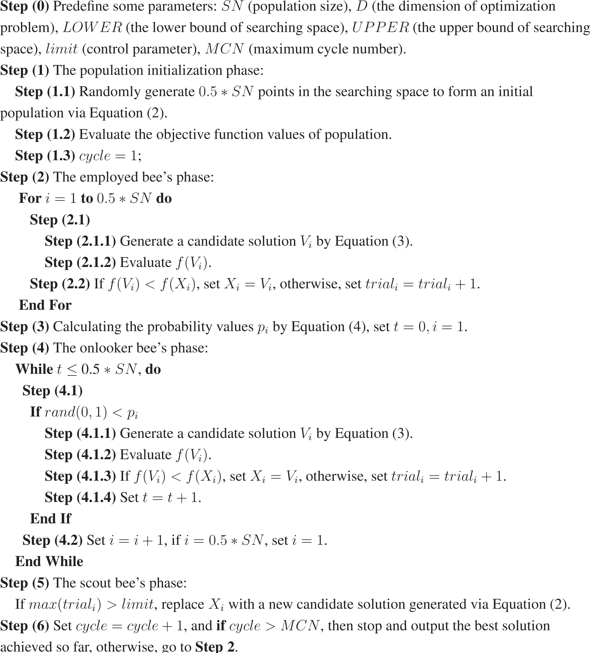
2.2.6. Framework of the Standard Artificial Bee Colony Algorithm

Based on the above introduction, the framework of the standard artificial bee colony algorithm can be given as below:
Algorithm 1:. Framework of the standard artificial bee colony algorithm.
Entropy 17 00692f7

3. Problem Formulation

Consider the following fractional-order chaotic system:
0 D t α Y ( t ) = f ( Y ( t ) , Y 0 , θ ) ,
where Y (t) = (y1(t), y2(t),⋯, yn (t))TRn denotes the state vector of System (6), Y0 = Y (0) denotes the initial value, θ = (θ1, θ2,⋯, θn)T denotes the set of original systematic parameters and α = (α1, α2,⋯, αn)(0 < αi < 1, i = 1, 2,⋯, n) are the fractional derivative orders. Additionally, f(Y (t), Y0, θ) = (f1(Y (t), Y0, θ), f2(Y (t), Y0, θ),⋯, fn(Y (t), Y0, θ))T.
The corresponding estimated system can be written as:
0 D t α ˜ Y ˜ ( t ) = f ( Y ˜ ( t ) , Y 0 , θ ˜ ) ,
where Y ˜ ( t ) = ( y ˜ 1 ( t ) , y ˜ 2 ( t ) , , y ˜ n ( t ) ) T R n is the state vector of the estimated System (7), θ ˜ = ( θ ˜ 1 , θ ˜ 2 , θ ˜ n ) T is a set of estimated systematic parameters and α ˜ = ( α ˜ 1 , α ˜ 2 , α ˜ n ) T is the estimated fractional orders. Besides, Systems (6) and (7) have the same initial conditions Y0.
In general, to identify the fractional-order chaotic System (6), it can be transformed into a functional extrema model as follows:
J ( α ˜ , θ ˜ ) = arg min ( α ˜ , θ ˜ ) Ω F = arg min ( α ˜ , θ ˜ ) Ω k = 1 N Y k Y ˜ k 2 ,
where k = 1, 2,⋯, N is the sampling time point and N denotes the length of data used for parameter estimation. Yk and Y ˜ k respectively denote the state vector of the original System (6) and the estimated System (7) at time kh. h is the step size employed in the predictor-corrector approach for the numerical solutions of fractional differential equations [19]. ‖⋅‖ is the Euclid norm. Ω is the searching area admitted for parameters θ ˜, where fractional orders α ˜ are considered as special variables. The parameter identification of System (6) can be achieved by searching suitable θ ˜ and α ˜ in the searching space Ω, such that the objective function is minimized. In other words, the main task is to find the best combination of the independent variables of α ˜ and θ ˜ for the objective function.

4. A Modified Artificial Bee Colony Algorithm

In order to improve the convergence speed and accuracy of the standard ABC algorithm, some modifications in terms of the searching equations are proposed. Additionally, they are described in detail in the following subsections.

4.1. Two Modified Solution Searching Equations

To improve the performance of the standard ABC algorithm, one effective research trend is to investigate searching equations. So far, a variety of searching equations have been put forward [2024]. The most representative one is GABCproposed by Zhu and Kwong [21]. In this method, in order to improve the exploitation and make full use of the information of the gbest solution to guide the search of candidate solution, a modified searching equation enlightened by PSO is suggested as follows:
v i , j = x i , j + ϕ i , j ( x i , j x k , j ) + ψ i , j ( x b e s t , j x i , j ) ,
where the third term in the right-hand side of Equation (9) is a new added term called the gbest term, xbest,j is the j-th element of the global best solution and ψi,j is a uniform random number in [0, 1.5]. Nevertheless, based on the experiment results shown in [21], it can be found that the improvement of the algorithm is not notable.
Thus, owing to the poor performance of the above Equation (3) and Equation (9), two new searching equations are presented to be used by the employed and onlooker bees, separately. The two equations are written as below:
v i , j = x r 1 , j + λ ( x i , j x r 1 , j ) + μ ( x b e s t , j x r 1 , j ) ,
v i , j = x b e s t , j + p i ( x i , j x b e s t , j ) + ν ( x r 1 , j x r 2 , j ) ,
where xbest,j is the j-th element of the global best solution. Similar to PSO algorithms, xi,j denotes the j-th element of the best previous solution of employed bee i (i.e., the local-best position or its experience). r1 and r2 are distinct integers randomly selected from {1, 2,⋯, SN} and are also different from i and best. j ∈ {1, 2,⋯, n} is a randomly chosen index. pi represents the current probability of the i-th employed bee. λ, μ are a random number in the range [0, 1], and ν is a random number in the range [−1, 1].
From Equation (10), due to the first term, the new candidate solution is generated around Xr1, which is a randomly selected individual from the population. The randomly selected individual Xr1 can bring more information to the searching equation and avoid being trapped into the local optimum, which is good at exploration. Besides, despite the guidance of Xbest not being used in the first term, Equation (10) can also take full advantage of xi,j and Xbest in the latter two terms to drive the new candidate solution towards the current best solution, which can guarantee its convergence speed. Therefore, the last two terms of Equation (10) do well in the exploitation. Generally speaking, Equation (10) can keep the exploration and exploitation well balanced. However, because of the guidance of Xr1 in the first term, Equation (10) pays more attention to the exploration. According to [10], in the employed bee phase, the searching process focuses on the exploration, which is consistent with the emphasis of Equation (10). Therefore, Equation (10) is chosen as the searching equation for the employed bees.
In Equation (11), owing to the first term, the new candidate solution is generated around Xbest, which stands for the current global best solution. The current probability is introduced in the second term to make full use of the information of the current population to further enhance the exploitation. Thus, the first two terms have effects on the exploitation ability. In addition, to keep balance corresponding to the first two terms in Equation (11), the third term is recommended to improve the diversity of the population. To sum up, Equation (11) may be beneficial to not only the convergence, but also the diversity of the population. However, due to the guidance of Xbest in the first term, Equation (11) places more emphasis on the exploitation. According to [10], the onlooker bee phase concentrates on the exploitation, which is inconsistent with the emphasis of Equation (11). Therefore, Equation (11) is selected as the searching equation for the onlooker bees.

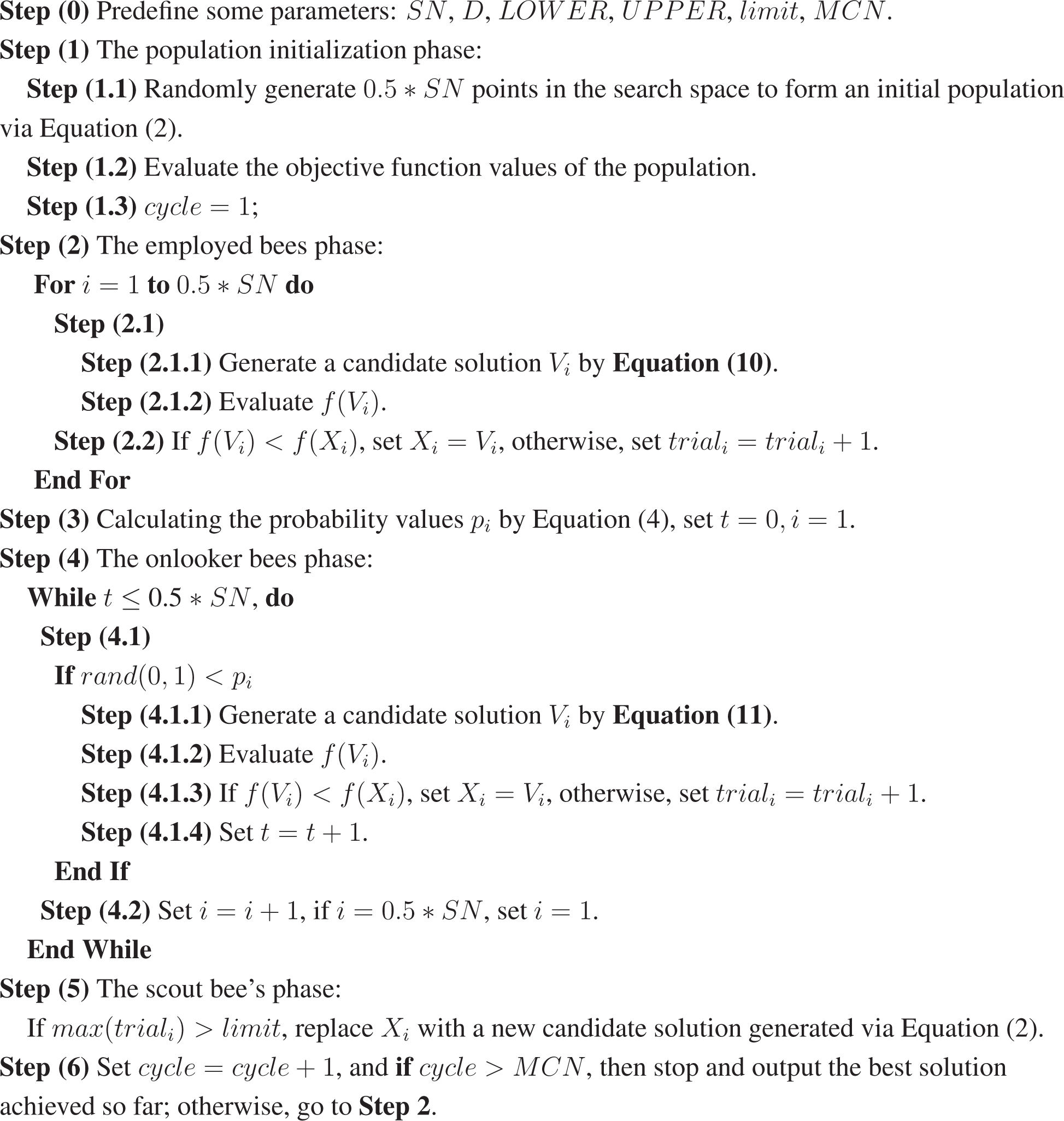
4.2. The Proposed Method
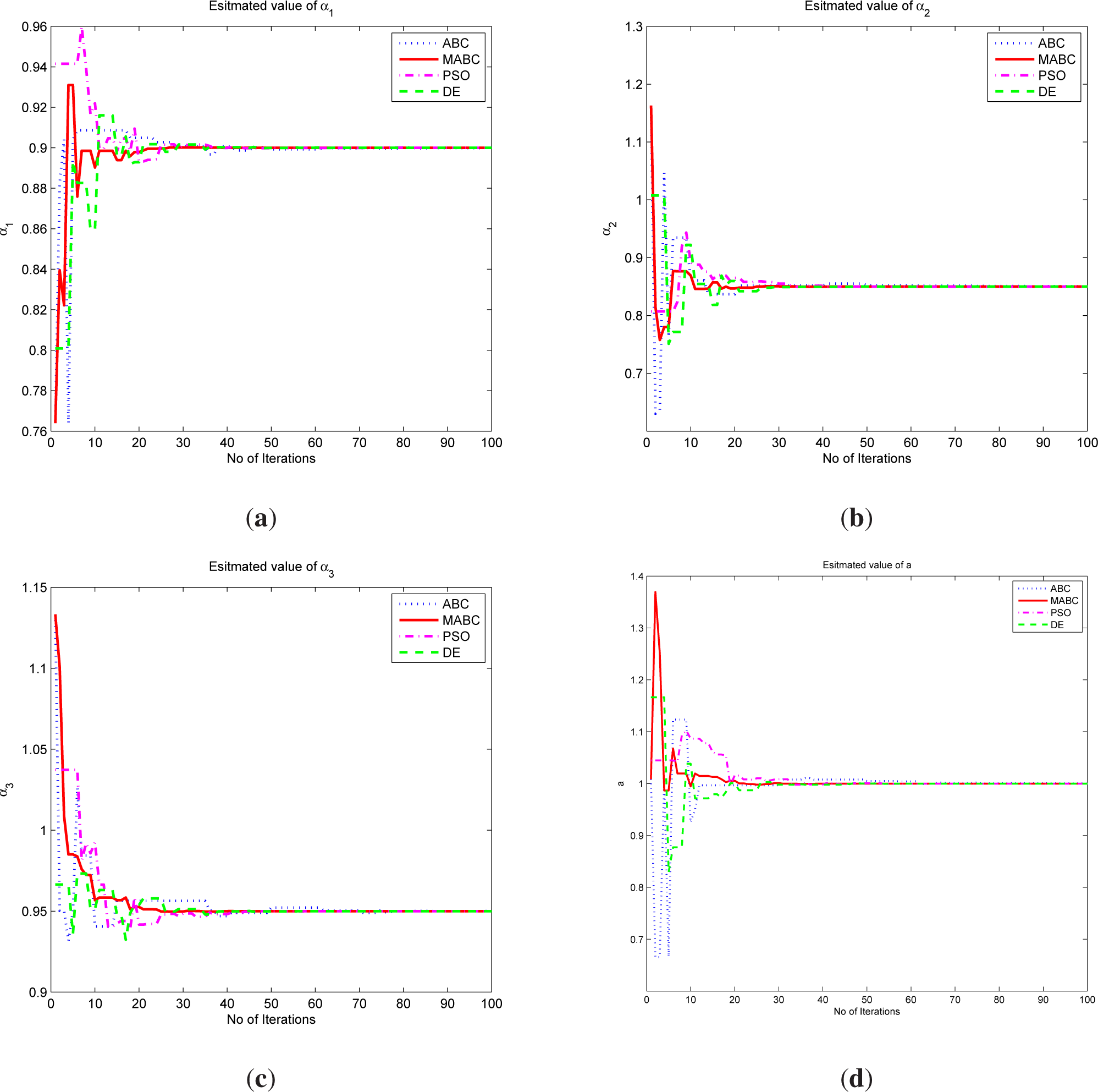
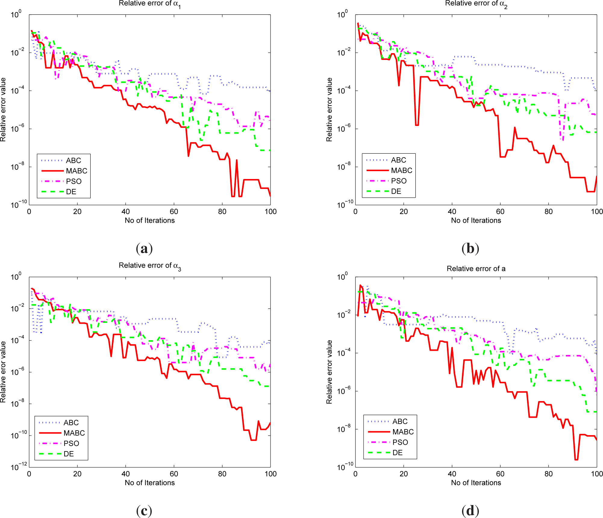
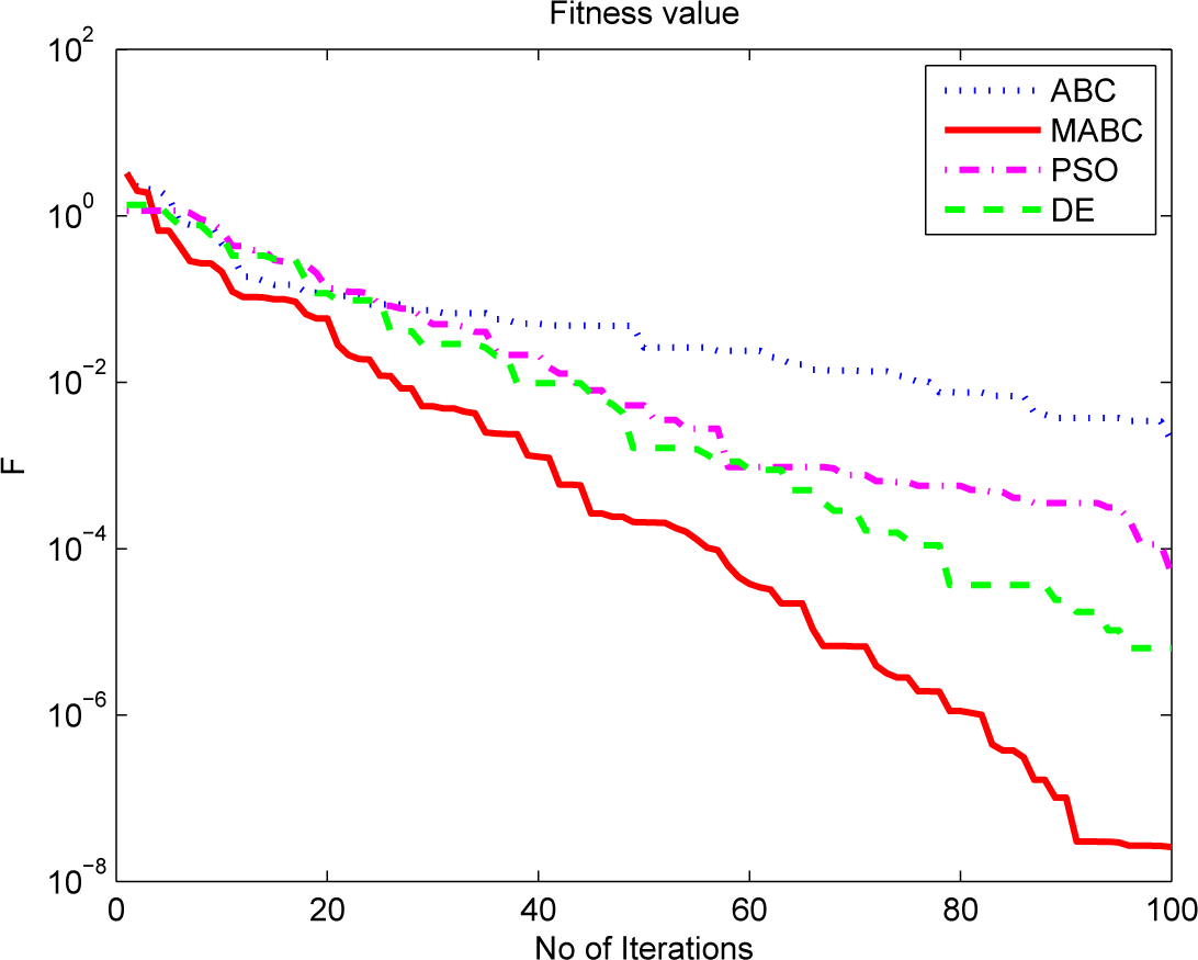
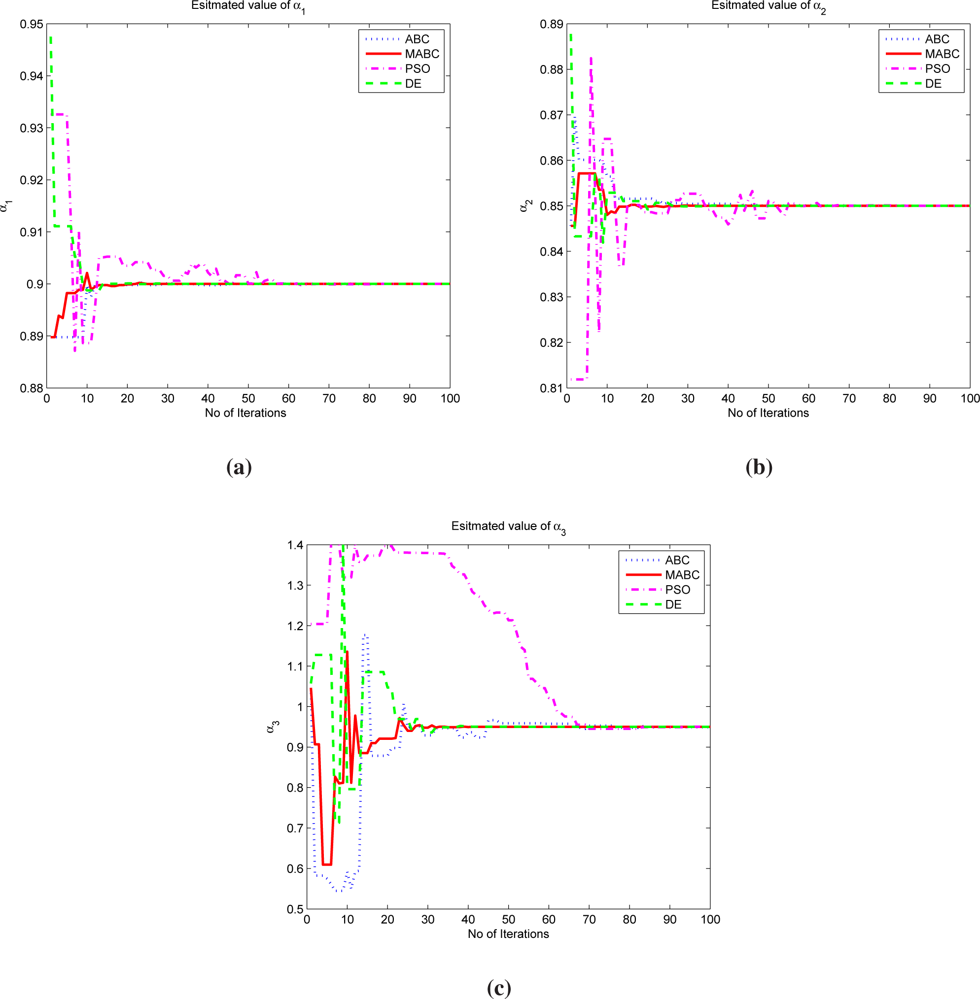
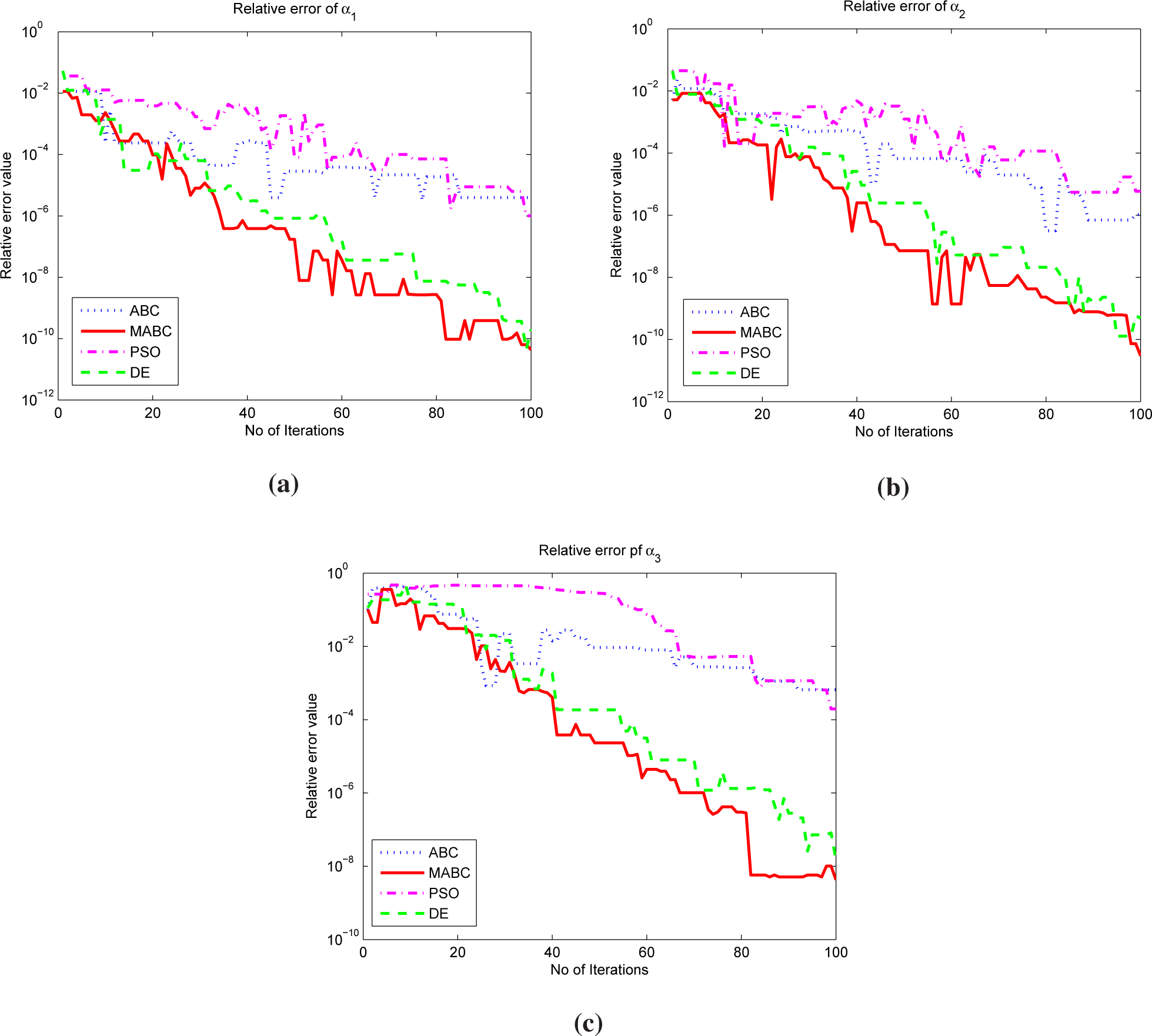
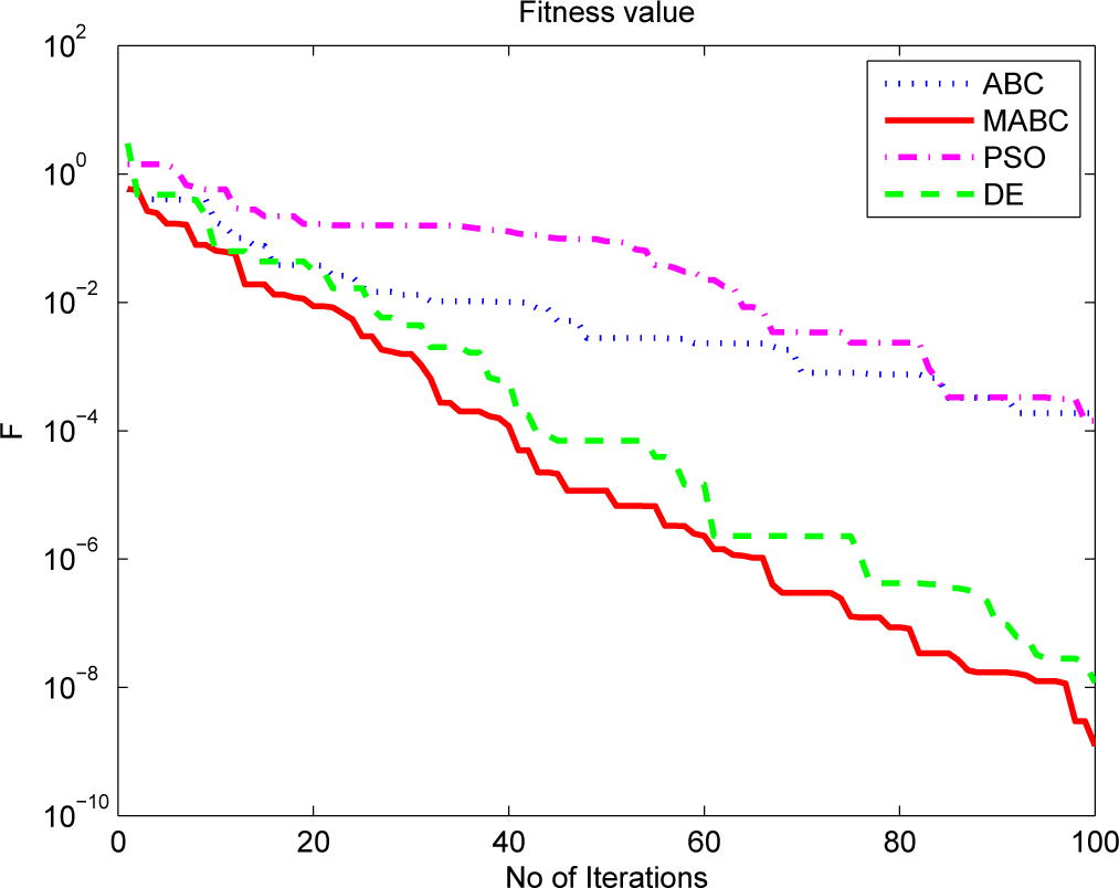
In view of the above, a new algorithm is proposed. Two new searching equations are proposed to generate new candidate solutions on the employed bee’s phase and onlooker bee’s phase, respectively. The pseudo-code of the modified ABC algorithm (here, we call it MABC) is given below:
Algorithm 2:. Framework of the modified ABC algorithm.
Entropy 17 00692f8

5. Simulations

To verify the effectiveness of the MABC algorithm, two typical fractional-order chaotic systems are chosen to test the performance. The simulations were done using MATLAB (Version 7.1, MathWorks, Natick, MA, USA) on an Intel(R) Core(TM) i5-3470 CPU, 3.2 GHz with 4 GB of RAM. In order to calculate the objective function, the number of samples is set as 300 and the step size is 0.01. As is well known, the larger the population and the maximum cycle number, the larger the probability of finding the global optimum. However, a larger population and maximum cycle number implies a larger number of function evaluations. In the following simulations, for the MABC, ABC, PSO and DE algorithms, the population size (SN) and maximum cycle number (MCN) are all set as: SN = 100, MCN = 100. Besides, for the MABC and ABC algorithms, according to [10], to make a fair comparison and have good searching ability, the control parameter limit is chosen as 15. For the parameters of the DE algorithm, according to [7], the scaling factor F = 0.5 is usually a good choice. If the parameter F is smaller, the population may converge prematurely. On the contrary, the convergence speed decreases. Besides, regarding the crossover rate CR, a large CR often speeds up the convergence. However, from a certain value upwards, the convergence speed may decrease or the population may also converge prematurely. A good choice for the crossover rate is a value between CR = 0.3 and CR = 0.9. In the following experiments, the parameters of DE are selected as: F = 0.5, CR = 0.7. For PSO, empirical results have shown that an inertia weight w = 0.7298 and cognitive and social factors with c1 = c2 = 1.49618 provide good convergent behavior [4,25]. Therefore, in the following simulation, the parameters for PSO are set as: w = 0.7298, c1 = c2 = 1.49618. To make a fair comparison, the searching spaces of the parameters are the same for all algorithms.
Example 1. The fractional-order economic system [26,27] is described as:
{ 0 D t α 1 x ( t ) = z ( t ) + ( y ( t ) a ) x ( t ) , 0 D t α 2 y ( t ) = 1 b y ( t ) x 2 ( t ) , 0 D t α 3 z ( t ) = x ( t ) c z ( t ) ,
when (a, b, c) = (1, 0.1, 1), (α1, α2, α3) = (0.90, 0.85, 0.95) and the initial point is (2, −1, 1), System (12) is chaotic. To show the performance of the MABC algorithm clearly, the true values of fractional orders α1, α2, α3 and systematic parameter a are assumed as unknown parameters, which need to be estimated. The searching spaces of the unknown parameters and orders are set as (α1, α2, α3, a) ∈ [0.1, 1.4] × [0.1, 1.4] × [0.1, 1.4] × [0.5, 1.5].
The statistical results of the best, the mean and the worst estimated parameters with the corresponding relative error values over 15 independent runs are shown in Table 1. From Table 1, it can be easily seen that the estimated value generated by the MABC algorithm is closer to the true parameter value, which means that it is more accurate than the standard ABC, PSO and DE algorithms. Besides, it can also be clearly found that the relative error values obtained by the MABC algorithm and marked with black are all smaller than those of the standard ABC, PSO and DE algorithms, which can further prove that the MABC algorithm has higher calculation accuracy. What is more, the best fitness value obtained by the MABC algorithm is better than those obtained by the standard ABC, PSO and DE algorithms.
The evolutionary curves of the parameters and fitness values estimated by the various algorithms are shown in Figures 13 in a single run. From Figures 13, it can be clearly seen that convergence processes of the parameters and fitness values of MABC algorithm are much better than other algorithms. The estimated parameters can be closer to the true values than the standard ABC, PSO and DE algorithms. Additionally, the relative error values and fitness values obtained by the MABC algorithm decline faster than the other algorithms. In other words, it can be concluded that the MABC algorithms can more efficiently identify a fractional-order economic system than the standard ABC algorithm, as well as the existing PSO and DE algorithms.
Example 2. The fractional-order Rössler system [26,28] is described as:
{ 0 D t α 1 x ( t ) = ( y ( t ) + z ( t ) ) , 0 D t α 2 y ( t ) = x ( t ) + a y ( t ) , 0 D t α 3 z ( t ) = b + z ( t ) ( x ( t ) c ) ,
when (a, b, c) = (0.5, 0.2, 10), (α1, α2, α3) = (0.90, 0.85, 0.95) and the initial point is (0.5, 1.5, 0.1), System (13) is chaotic. In this example, the fractional orders α1, α2, α3 are selected as unknown parameters to be estimated. The searching spaces of the unknown parameters are set as (α1, α2, α3) ∈ [0.1, 1.4] × [0.1, 1.4] × [0.1, 1.4].
To show the performance of MABC algorithm, the statistical results of the best, the mean and the worst estimated parameters by various algorithms over 15 independent runs are listed in Table 2. From Table 2, it can be seen that the MABC algorithm has more accurate results than those of the standard ABC, PSO and DE algorithms. Figures 46 depict the convergence profile of the evolutionary processes of the estimated parameters and the fitness values. From the figures, it can be seen that the MABC algorithm still can converge to the optimal solution more rapidly than the other algorithms.
Based on the above two examples, the proposed scheme is significantly better than all of the other listed algorithms, and it has a faster convergence speed and higher calculation accuracy in estimating the unknown fractional orders and systematic parameters of fractional-order systems.

6. Conclusions

In this paper, the parameter estimation of fractional-order chaotic systems is converted to an optimization problem from the prospect of optimization. A modified artificial bee colony algorithm is proposed to solve the optimization problem via a functional extrema model. In simulations, the proposed method is employed to identify two typical fractional-order chaotic systems. It is shown that, for the given parameter configurations and maximum number of iterations, the modified ABC algorithm could estimate the unknown fractional orders and parameters of the uncertain fractional-order chaotic systems more rapidly, more accurately and more stably than standard the ABC, PSO and DE algorithms. Additionally, the proposed method can avoid the design of the parameter update law in the synchronization analysis of the fractional-order chaotic systems with unknown parameters. Furthermore, although this paper is mainly concentrated on the parameter estimation problem of the fractional-order chaotic systems, the proposed method is also a useful tool for the study of various numerical optimization problems in physics and other related areas.

Acknowledgments

This work is supported by the National Nature Science Foundation of China (No. 11371049).

Author Contributions

Wei Hu and Yongguang Yu proposed and designed the research; Wei Hu performed the simulations and wrote the paper; Wei Hu, Yongguang Yu and Sha Wang analyzed the simulation results. All authors have read and approved the final manuscript.

Conflicts of Interest

The authors declare no conflict of interest.

References

  1. Kilbas, A.A.A.; Srivastava, H.M.; Trujillo, J.J. Theory and Applications of Fractional Differential Equations; Elsevier: Amsterdam, the Netherlands, 2006. [Google Scholar]
  2. Arena, P.; Caponetto, R.; Fortuna, L.; Porto, D. Nonlinear Noninteger Order Circuits and Systems—An Introduction; World Scientific: Singapore, Singapore, 2000. [Google Scholar]
  3. Rivero, M.; Rogosin, S.V.; Tenreiro Machado, J.A.; Trujillo, J.J. Stability of fractional order systems. Math. Probl. Eng. [CrossRef]
  4. Kennedy, J.; Eberhart, R. Particle swarm optimization, Proceedings of IEEE International Conference on Neural Networks, Piscataway, NJ, USA, 27 November–1 December 1995; pp. 1942–1948.
  5. Yuan, L.G.; Yang, Q.G. Parameter identification and synchronization of fractional-order chaotic systems. Commun. Nonlinear Sci. Numer. Simul. 2012, 17, 305–316. [Google Scholar]
  6. Alfi, A.; Modares, H. System identification and control using adaptive particle swarm optimization. Appl. Math. Model. 2011, 35, 1210–1221. [Google Scholar]
  7. Storn, R.; Price, K. Differential evolution—a simple and efficient heuristic for global optimization over continuous spaces. J. Global Optim 1997, 11, 341–359. [Google Scholar]
  8. Gao, F.; Fei, F.X.; Lee, X.J.; Tong, H.Q.; Deng, Y.F.; Zhao, H.L. Inversion mechanism with functional extrema model for identification incommensurate and hyper fractional chaos via differential evolution. Expert Syst. Appl. 2014, 41, 1915–1927. [Google Scholar]
  9. Tang, Y.G.; Zhang, X.Y.; Hua, C.C.; Li, L.X.; Yang, Y.X. Parameter identification of commensurate fractional-order chaotic system via differential evolution. Phys. Lett. A. 2012, 376, 457–464. [Google Scholar]
  10. Karaboga, D. An Idea Based on Honey Bee Swarm for Numerical Optimization; Technical Report-TR06; Erciyes University: Kayseri, Turkey, October 2005. [Google Scholar]
  11. Karaboga, D.; Akay, B. A comparative study of artificail bee colony algorithm. Appl. Math. Comput. 2009, 214, 108–132. [Google Scholar]
  12. Karaboga, D.; Akay, B. On the performance of artificial bee colony (ABC) algorithm. Appl. Soft Comput. 2008, 8, 687–697. [Google Scholar]
  13. Biswas, S.; Das, S.; Debchoudhury, S.; Kundu, S. Co-evolving bee colonies by forager migration: A multi-swarm based Artificial Bee Colony algorithm for global search space. Appl. Math. Comput. 2014, 232, 216–234. [Google Scholar]
  14. Li, X.T.; Yin, M.H. Parameter estimation for chaotic systems by hybrid differential evolution algorithm and artificial bee colony algorithm. Nonlinear Dyn 2014, 77, 61–71. [Google Scholar]
  15. Zhang, W.; Wang, N.; Yang, S.P. Hybrid artificial bee colony algorithm for parameter estimation of proton exchange membrane fuel cell. Int. J. Hydrog. Energy. 2013, 38, 5796–5806. [Google Scholar]
  16. Tang, K.S.; Man, K.F.; Kwong, S.; He, Q. Genetic algorithms and their applications. IEEE Signal Proc. Mag. 1996, 13, 22–37. [Google Scholar]
  17. Price, K.V.; Storn, R.M.; Lampinen, J.A. Differential Evolution: A Practial Approach to Global Optimization; Springer: Berlin/Heidelberg, Germany, 2005. [Google Scholar]
  18. Podlubny, I. Fractional Differential Equations; Academic Press: San Diego, CA, USA, 1999. [Google Scholar]
  19. Diethelm, K.; Ford, N.J.; Freed, A.D. A predictor-corrector approach for the numerical solution of fractional differential equations. Nonlinear Dyn 2002, 29, 3–22. [Google Scholar]
  20. Gao, W.F.; Liu, S.Y. A modified artificial bee colony algorithm. Comput. Oper. Res. 2012, 39, 687–697. [Google Scholar]
  21. Zhu, G.P.; Kwong, S. Gbest-guided artificial bee colony algorithm for numerical function optimization. Appl. Math. Comput. 2010, 217, 3166–3173. [Google Scholar]
  22. Gao, W.F.; Liu, S.Y.; Huang, L.L. A global best artificial bee colony algorithm for global optimization. J. Comput. Appl. Math. 2012, 236, 2741–2753. [Google Scholar]
  23. Gao, W.F.; Liu, S.Y.; Huang, L.L. A novel artificial bee colony algorithm based on modified search equation and orthogonal learning. IEEE Trans. Cybern. 2013, 43, 1011–1024. [Google Scholar]
  24. Banharnsakun, A.; Achalakul, T.; Sirinaovakul, B. The best-so-far selection in artificial bee colony algorithm. Appl. Soft Comput 2010, 11, 2888–2901. [Google Scholar]
  25. Eberhart, R.C.; Shi, Y. Comparing inertia weights and constriction factors in particle swarm optimization, Proceedings of the 2000 Congress on Evolutionary Computation, San Diego, CA, USA, 16–19 July 2000; pp. 84–88.
  26. Petráš, I. Fractional-order chaotic systems. In Fractional-Order Nonlinear Systems: Modeling, Analysis and Simulation; Spring: Berlin/Heidelberg, Germany, 2011; pp. 103–184. [Google Scholar]
  27. Chen, W.C. Nonlinear dynamics and chaos in a fractional-order financial system. Chaos Soliton. Fract. 2008, 36, 1305–1314. [Google Scholar]
  28. Li, C.; Chen, G.R. Chaos and hyperchaos in the fractional-order Rössler equations. Physica A 2004, 341, 55–61. [Google Scholar]
Figure 1. Estimated parameter values with various algorithms on a fractional-order economic system.
Entropy 17 00692f1
Figure 2. Relative error values with various algorithms on a fractional-order economic system.
Entropy 17 00692f2
Figure 3. Best fitness values with various algorithms on a fractional-order economic system.
Entropy 17 00692f3
Figure 4. Estimated parameter values with various algorithms on a fractional-order Rössler system.
Entropy 17 00692f4
Figure 5. Relative error values with various algorithms on a fractional-order Rössler system.
Entropy 17 00692f5
Figure 6. Best fitness values with various algorithms on a fractional-order Rössler system.
Entropy 17 00692f6
Table 1. Simulation results of various algorithm for System (12) over 15 independent runs. MABC, modified ABC; DE, differential evolution.
AlgorithmABCMABCPSODE
Bestα10.899997107511390.900000000007790.900000087340440.90000000839266
| α 1 0.90 | 0.900.000002890.000000000007790.00000008730.0000000839
α20.850003404257670.849999999748200.849998498346070.85000001554904
| α 2 0.85 | 0.850.000003400.0000000002520.000001500.0000000155
α30.950001095566630.950000000066060.949998159944240.94999999728649
| α 3 0.95 | 0.950.000001100.00000000006610.000001840.00000000271
a1.000008244467131.000000000016850.999999408899940.99999991725828
| α 1.00 | 1.000.000008240.00000000001690.0000005910.0000000827
F0.0001090.000000003810.00004960.00000150

Meanα10.899998988390060.900000000096920.900003911813210.90000002685242
| α 1 0.90 | 0.900.000001010.00000000009690.000003910.0000000269
α20.849992000414400.849999999957730.849995849874090.85000004254726
| α 2 0.85 | 0.850.0000080.00000000004230.000004150.0000000425
α30.950013654333650.949999999791060.949999458174900.94999990594634
| α 3 0.95 | 0.950.00001370.0000000002090.0000005420.0000000941
a0.999999601821300.999999999070770.999988424417331.00000002104131
| α 1.00 | 1.000.0000003980.0000000009290.00001160.0000000210
F0.001100.00000001870.0001360.00000441

Worstα10.899867590493170.899999997542740.900018510000840.90000037757625
| α 1 0.90 | 0.900.0001320.000000002460.00001850.000000378
α20.850244400080370.850000007092500.849981255615420.85000066521416
| α 2 0.85 | 0.850.0002440.000000007090.00001870.000000665
α30.950211287076720.949999998459070.949969093753710.94999907973644
| α 3 0.95 | 0.950.0002110.000000001540.00003090.000000920
a1.000431672624470.999999996472420.999932456424780.99999938116949
| α 1.00 | 1.000.0004320.000000003530.00006750.000000619
F0.002530.00000006260.0003770.00000982
Table 2. Simulation results of various algorithm for System (13) over 15 independent runs.
AlgorithmABCMABCPSODE
Bestα10.899999883364650.900000000000570.899999768008250.89999999997794
| α 1 0.90 | 0.900.0000001170.0000000000005650.0000002320.0000000000221
α20.849999730458740.849999999999370.849998560190880.85000000023856
| α 2 0.85 | 0.850.0000002700.0000000000006350.000001440.000000000239
α30.949988116212000.950000000055660.950125182897190.95000000987768
| α 3 0.95 | 0.950.00001190.00000000005570.0001250.00000000988
F0.00006660.00000000004050.00008280.0000000120

Meanα10.900002275417880.899999999977840.899995811661100.89999999996680
| α 1 0.90 | 0.900.000002280.00000000002220.000004190.0000000000332
α20.850000372331120.850000000043180.850010367461140.84999999991562
| α 2 0.85 | 0.850.0000003720.00000000004320.00001040.0000000000844
α30.950376641056730.950000000563340.949573642044930.94999999450775
| α 3 0.95 | 0.950.0003770.0000000005630.0004260.00000000549
F0.0003950.000000003280.0005570.0000000234

Worstα10.900020812049870.899999999898720.899947776222300.90000000092049
| α 1 0.90 | 0.900.00002080.0000000001010.00005220.000000000920
α20.850020336752380.850000000492230.850129935221340.84999999861606
| α 2 0.85 | 0.850.00002030.0000000004920.0001300.00000000138
α30.952051651779200.950000035057320.943528721375210.94999989275506
| α 3 0.95 | 0.950.002050.00000003510.006470.000000107
F0.0007810.00000001160.002790.0000000383

