
Yangtze River Basin Environmental Regulation Efficiency Based on the Empirical Analysis of 97 Cities from 2005 to 2016


Abstract
:1. Introduction
2. Methodology
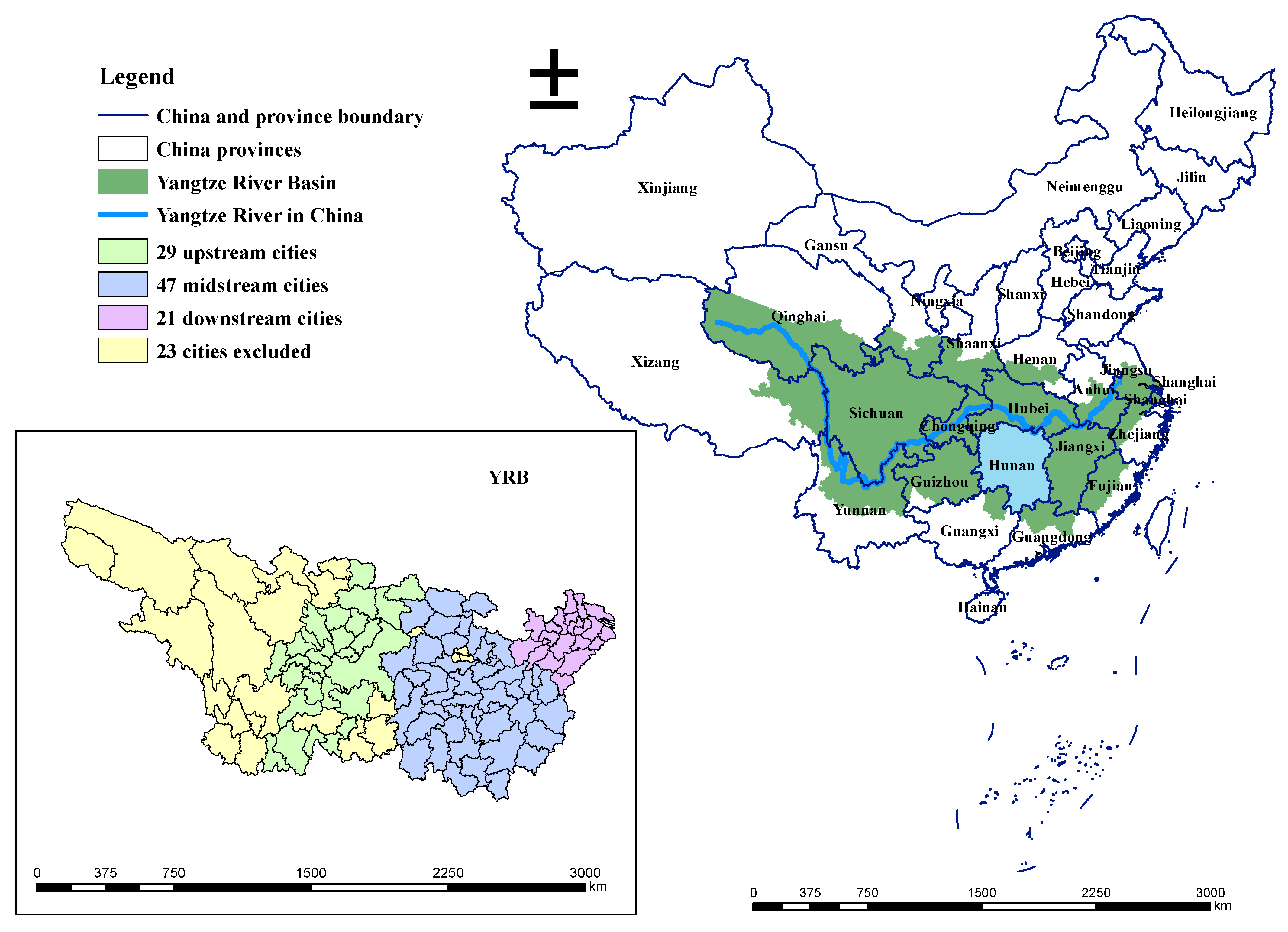
2.1. Study Area
2.2. The SE-SBM Model
2.3. DEA–Malmquist Index
3. Statistical Datasets
4. Results
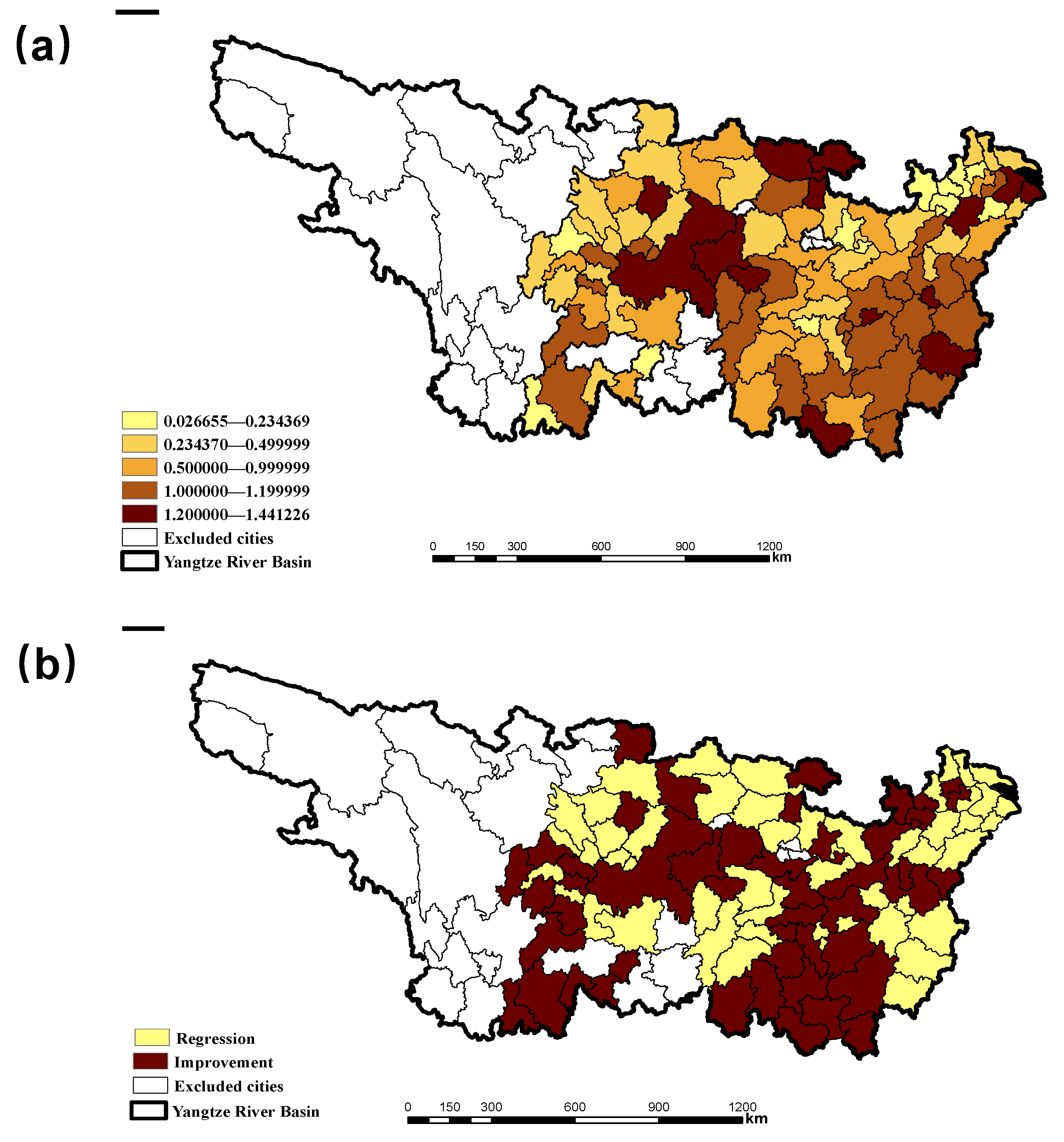
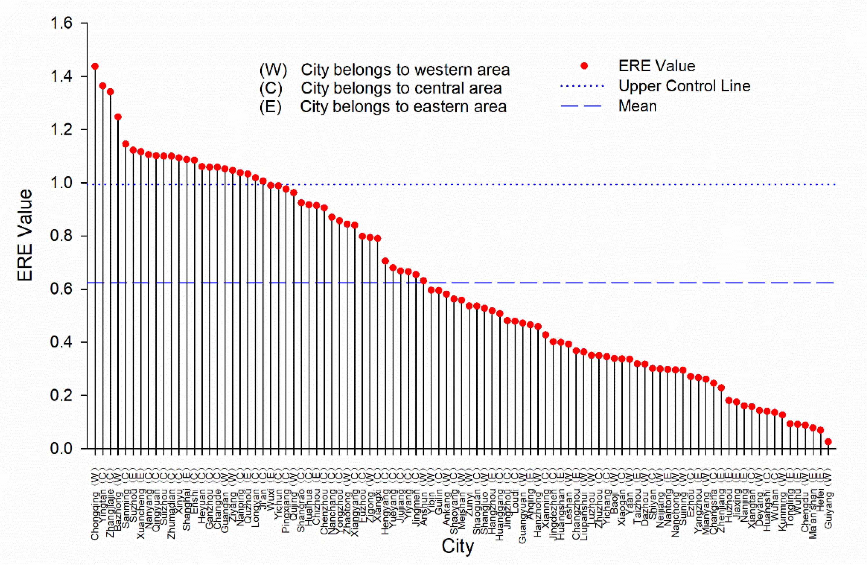
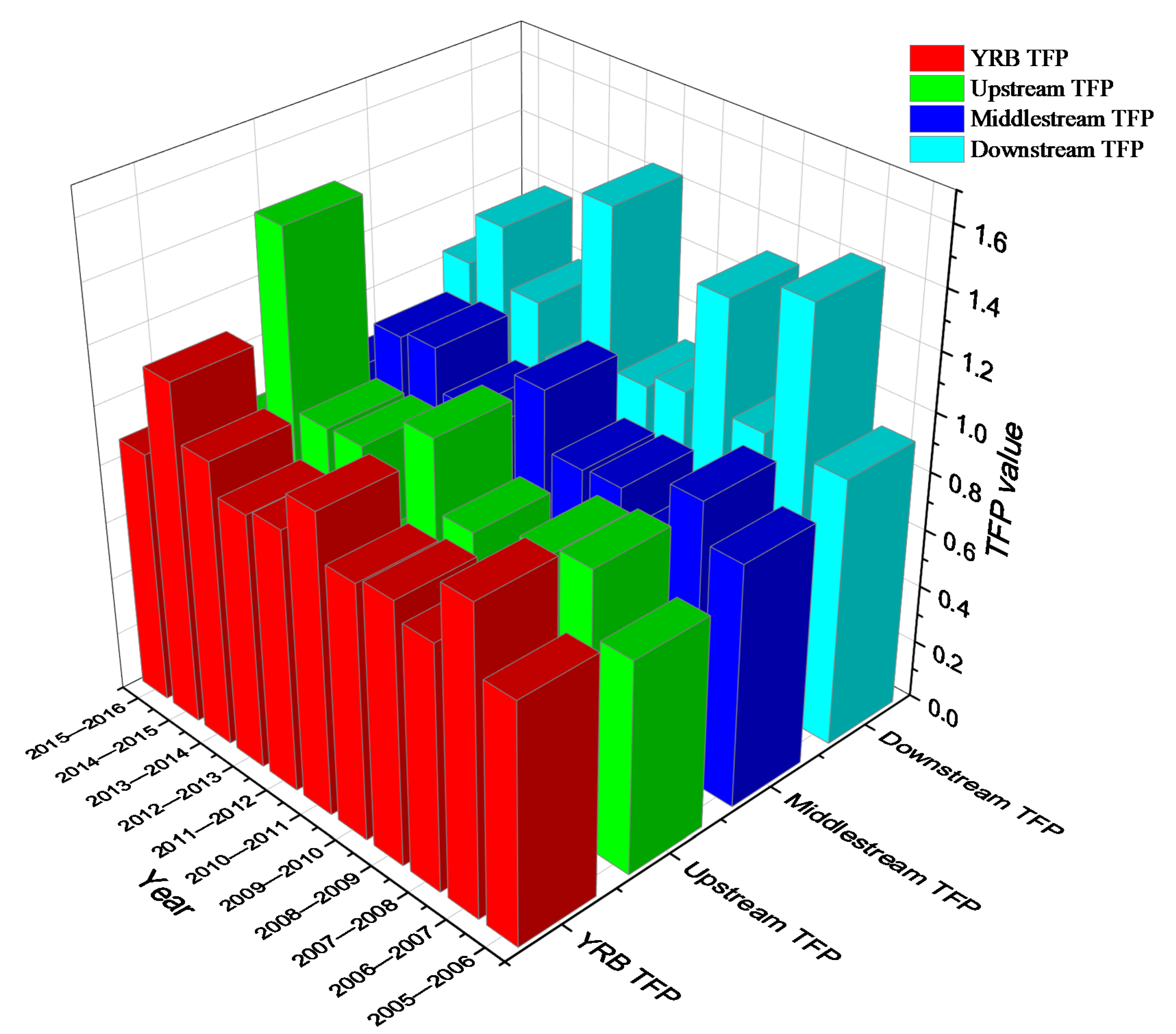
4.1. Yangtze River Basin Environmental Regulation Efficiency
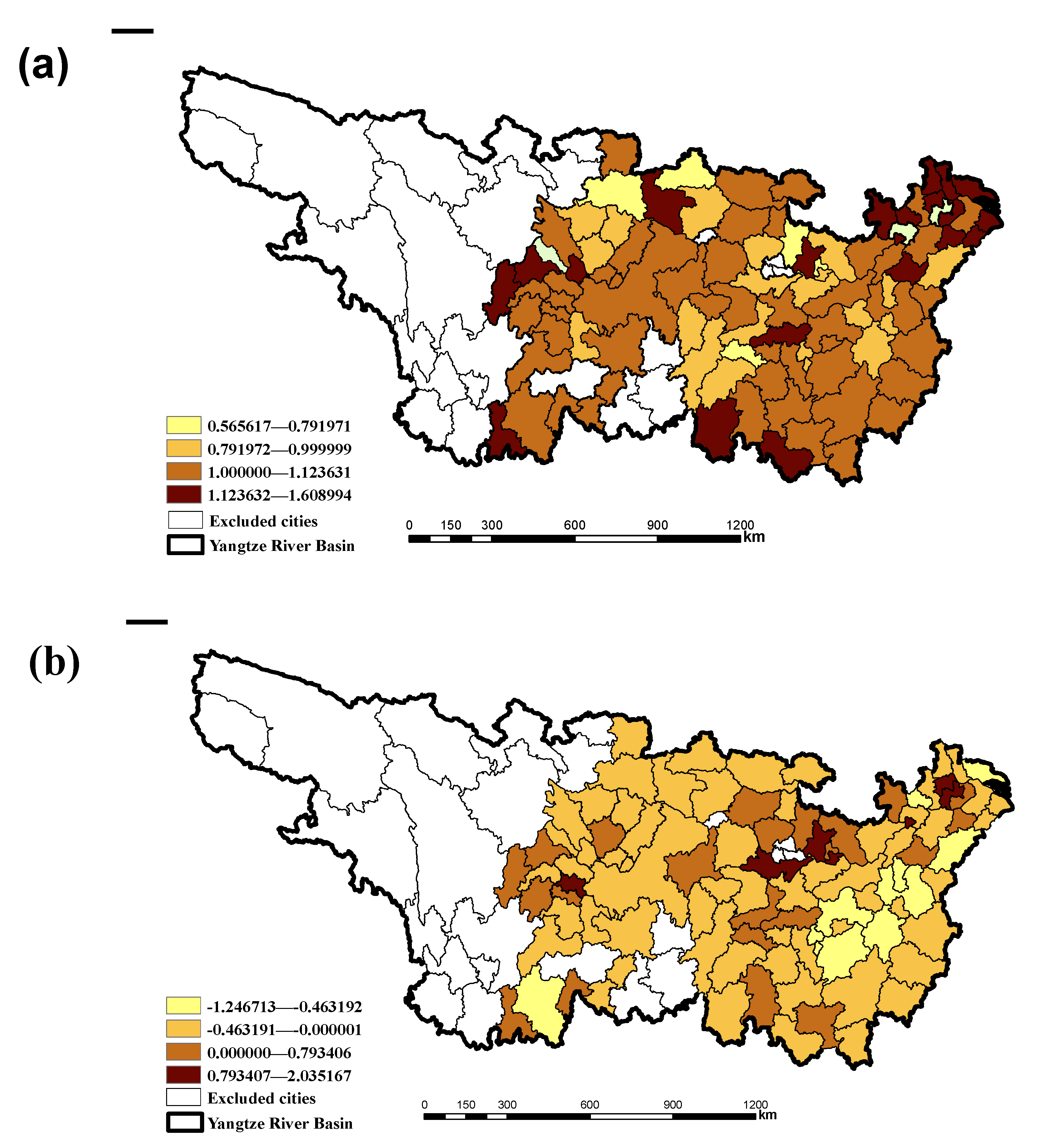
4.2. DEA–Malmquist Index
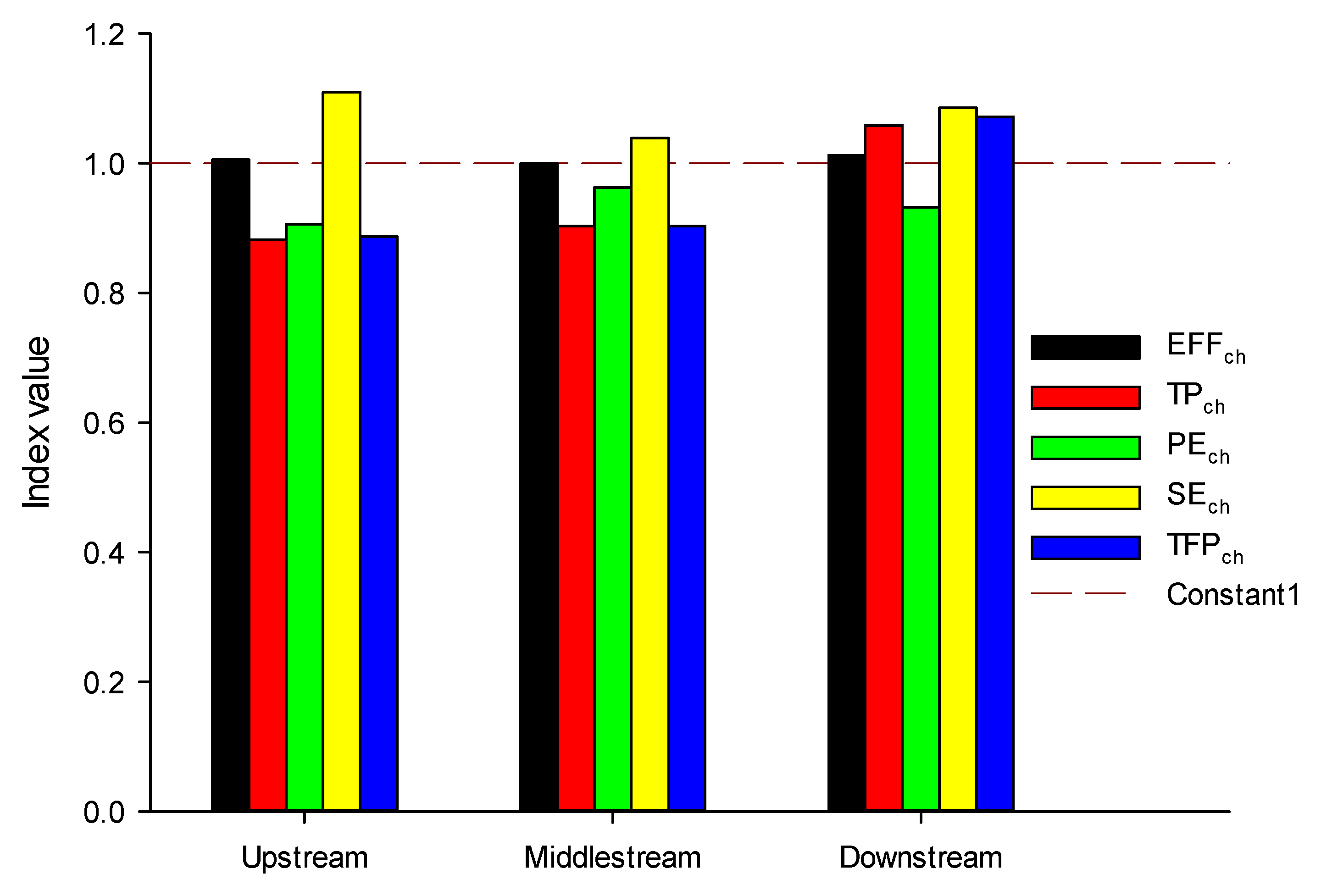
4.3. TFP Decomposition
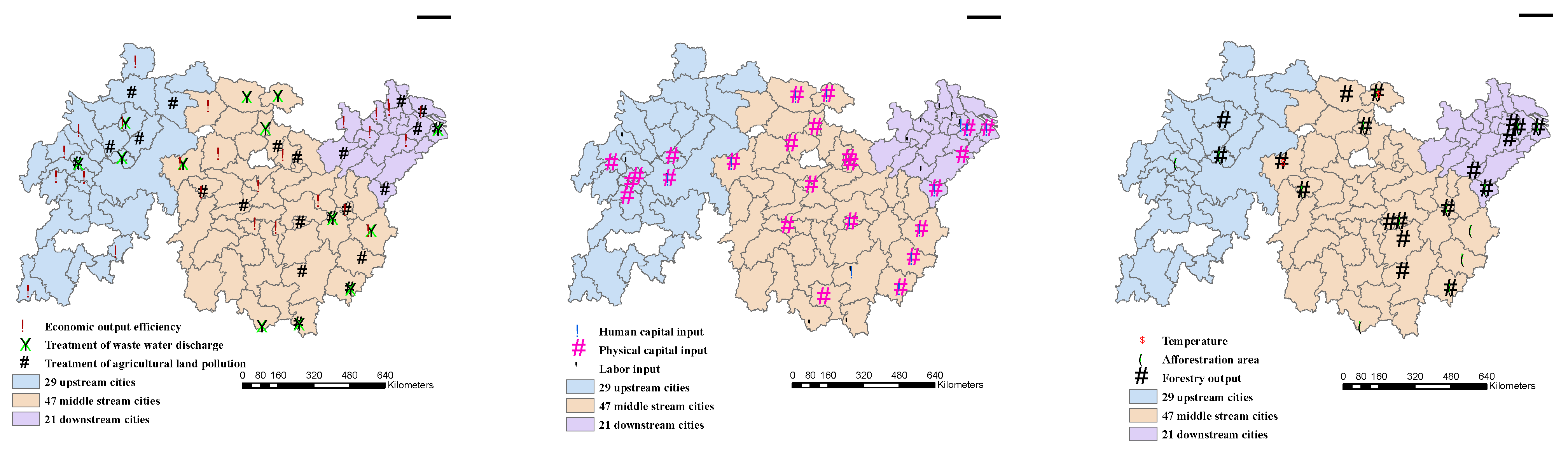
4.4. Slack Analysis Based on SE-SBM Model
5. Conclusions and Recommendations
Author Contributions
Funding
Institutional Review Board Statement
Informed Consent Statement
Data Availability Statement
Conflicts of Interest
Appendix A. ERE of 97 cities in YRB from 2005 to 2016

| City | 2005 | 2006 | 2007 | 2008 | 2009 | 2010 | 2011 | 2012 | 2013 | 2014 | 2015 | 2016 | Average |
|---|---|---|---|---|---|---|---|---|---|---|---|---|---|
| Changsha | 0.11 | 0.13 | 0.15 | 0.07 | 0.14 | 0.19 | 0.17 | 0.18 | 0.34 | 1.01 | 1.01 | 1.01 | 0.38 |
| Zhuzhou | 0.20 | 0.24 | 0.41 | 0.26 | 0.35 | 0.45 | 0.41 | 0.39 | 0.36 | 0.41 | 0.36 | 0.46 | 0.36 |
| Xiangtan | 0.19 | 0.16 | 0.15 | 0.05 | 0.12 | 0.11 | 0.17 | 0.19 | 0.18 | 0.23 | 0.25 | 0.23 | 0.17 |
| Hengyang | 0.52 | 1.04 | 1.02 | 1.01 | 1.01 | 0.76 | 0.44 | 0.48 | 0.51 | 0.56 | 0.58 | 1.00 | 0.74 |
| Shaoyang | 0.77 | 1.00 | 0.60 | 0.28 | 0.47 | 0.53 | 0.59 | 0.57 | 0.50 | 0.58 | 0.49 | 0.63 | 0.59 |
| Yueyang | 0.70 | 0.78 | 0.82 | 0.57 | 0.49 | 0.52 | 0.64 | 0.64 | 0.64 | 0.72 | 0.79 | 1.00 | 0.69 |
| Changde | 1.15 | 1.05 | 1.07 | 1.06 | 1.07 | 1.05 | 1.05 | 1.03 | 1.03 | 1.05 | 1.05 | 1.04 | 1.06 |
| Zhangjiajie | 1.27 | 1.25 | 1.20 | 1.30 | 1.24 | 1.27 | 1.33 | 1.39 | 1.49 | 1.45 | 1.44 | 1.50 | 1.34 |
| Yiyang | 1.01 | 0.77 | 0.72 | 0.38 | 0.58 | 0.70 | 0.74 | 0.63 | 0.27 | 0.66 | 1.01 | 1.00 | 0.71 |
| Chenzhou | 0.60 | 0.73 | 1.00 | 1.01 | 0.57 | 1.01 | 1.00 | 1.07 | 1.01 | 1.05 | 1.02 | 1.02 | 0.92 |
| Yongzhou | 0.68 | 0.63 | 1.00 | 0.47 | 0.58 | 1.06 | 1.03 | 1.05 | 1.00 | 1.05 | 1.04 | 1.08 | 0.89 |
| Huaihua | 1.07 | 1.02 | 1.05 | 1.03 | 0.75 | 0.72 | 1.01 | 1.02 | 0.69 | 1.01 | 0.77 | 1.00 | 0.93 |
| Loudi | 1.02 | 1.06 | 1.02 | 1.02 | 0.37 | 0.39 | 0.50 | 0.29 | 0.26 | 0.26 | 0.27 | 0.33 | 0.57 |
| Xiangxi | 1.11 | 1.13 | 1.01 | 0.26 | 0.44 | 0.52 | 1.10 | 1.05 | 1.03 | 1.01 | 0.66 | 1.01 | 0.86 |
| Nanchang | 1.03 | 1.03 | 1.04 | 1.02 | 1.04 | 1.04 | 1.05 | 1.05 | 1.06 | 1.05 | 1.05 | 0.12 | 0.96 |
| Jingdezhen | 0.23 | 0.34 | 0.49 | 0.36 | 0.34 | 0.26 | 0.40 | 0.40 | 0.42 | 0.59 | 1.01 | 0.35 | 0.43 |
| Pingxiang | 1.07 | 1.04 | 1.04 | 1.01 | 1.05 | 1.05 | 1.04 | 1.05 | 1.05 | 1.06 | 1.04 | 0.46 | 1.00 |
| Jiujiang | 0.43 | 0.44 | 1.03 | 0.50 | 0.67 | 0.55 | 0.62 | 0.59 | 1.02 | 1.03 | 1.03 | 0.55 | 0.71 |
| Xinyu | 1.05 | 1.07 | 1.07 | 1.00 | 1.07 | 1.16 | 1.18 | 1.13 | 1.12 | 1.13 | 1.14 | 1.01 | 1.09 |
| Yingtan | 1.22 | 1.78 | 1.35 | 1.34 | 1.37 | 1.28 | 1.37 | 1.41 | 1.48 | 1.40 | 1.28 | 1.17 | 1.37 |
| Ganzhou | 1.01 | 1.07 | 1.05 | 1.09 | 1.06 | 1.06 | 1.04 | 1.07 | 1.07 | 1.09 | 1.07 | 1.03 | 1.06 |
| Ji’an | 0.73 | 1.09 | 1.02 | 1.00 | 1.05 | 1.02 | 1.03 | 1.12 | 1.08 | 1.11 | 1.14 | 0.78 | 1.01 |
| Yichun | 0.68 | 1.02 | 1.12 | 1.06 | 1.06 | 1.07 | 1.05 | 1.05 | 1.05 | 1.03 | 1.04 | 0.74 | 1.00 |
| Fuzhou | 0.70 | 1.00 | 1.02 | 1.00 | 1.00 | 0.64 | 1.00 | 0.83 | 0.71 | 0.68 | 0.66 | 0.55 | 0.82 |
| Shangrao | 0.51 | 1.01 | 1.05 | 1.00 | 1.05 | 1.05 | 1.02 | 1.01 | 0.86 | 1.01 | 1.01 | 0.72 | 0.94 |
| Nanjing | 0.23 | 0.24 | 0.23 | 0.20 | 0.18 | 0.12 | 0.10 | 0.13 | 0.12 | 0.16 | 0.16 | 0.15 | 0.17 |
| Wuxi | 1.05 | 1.09 | 1.06 | 1.03 | 1.03 | 1.01 | 0.57 | 1.01 | 1.04 | 1.05 | 1.04 | 1.04 | 1.00 |
| Changzhou | 0.21 | 0.19 | 1.01 | 1.01 | 1.06 | 1.08 | 0.08 | 0.16 | 0.10 | 0.11 | 1.01 | 1.00 | 0.58 |
| Suzhou | 1.12 | 1.09 | 1.10 | 1.08 | 1.08 | 1.11 | 1.17 | 1.18 | 1.14 | 1.14 | 1.13 | 1.11 | 1.12 |
| Nantong | 0.26 | 0.32 | 0.39 | 0.31 | 0.29 | 0.28 | 0.22 | 0.26 | 0.25 | 0.30 | 0.53 | 0.26 | 0.31 |
| Yangzhou | 0.40 | 0.41 | 0.31 | 0.15 | 0.28 | 0.41 | 0.31 | 0.30 | 0.23 | 0.18 | 0.18 | 0.19 | 0.28 |
| Zhenjiang | 0.24 | 0.22 | 0.26 | 0.12 | 0.23 | 0.22 | 0.20 | 0.23 | 0.35 | 0.28 | 0.23 | 0.25 | 0.23 |
| Taizhou | 0.59 | 1.00 | 0.48 | 1.10 | 0.31 | 0.24 | 0.22 | 0.26 | 0.19 | 0.17 | 0.16 | 0.16 | 0.41 |
| Shanghai | 1.11 | 1.10 | 1.10 | 1.10 | 1.09 | 1.09 | 1.08 | 1.08 | 1.07 | 1.07 | 1.07 | 1.07 | 1.09 |
| Hangzhou | 1.11 | 1.11 | 1.11 | 1.10 | 1.11 | 1.07 | 0.29 | 0.26 | 0.25 | 0.20 | 0.22 | 0.26 | 0.67 |
| Jiaxing | 1.03 | 1.03 | 1.02 | 0.17 | 0.10 | 0.05 | 0.05 | 0.06 | 0.05 | 0.07 | 0.09 | 1.01 | 0.39 |
| Huzhou | 0.28 | 0.22 | 0.11 | 0.02 | 0.10 | 0.34 | 0.23 | 0.33 | 0.31 | 0.29 | 0.15 | 0.25 | 0.22 |
| Quzhou | 1.03 | 1.04 | 1.05 | 1.01 | 1.03 | 1.02 | 1.01 | 1.03 | 1.03 | 1.01 | 1.02 | 1.13 | 1.03 |
| Sanming | 1.19 | 1.14 | 1.13 | 1.12 | 1.18 | 1.18 | 1.14 | 1.12 | 1.17 | 1.13 | 1.11 | 1.14 | 1.15 |
| Nanping | 1.05 | 1.06 | 1.05 | 1.06 | 1.06 | 1.04 | 1.05 | 1.03 | 1.01 | 1.01 | 1.01 | 1.02 | 1.04 |
| Longyan | 1.05 | 1.03 | 1.01 | 1.02 | 1.03 | 1.02 | 1.01 | 1.01 | 1.01 | 1.01 | 1.01 | 1.02 | 1.02 |
| Guilin | 0.42 | 0.49 | 0.50 | 0.56 | 1.00 | 0.58 | 0.41 | 1.36 | 0.41 | 1.11 | 0.48 | 0.49 | 0.65 |
| Hefei | 0.11 | 0.02 | 0.02 | 0.04 | 0.02 | 0.03 | 0.02 | 0.12 | 0.23 | 0.26 | 0.25 | 0.29 | 0.12 |
| Wuhu | 0.02 | 0.02 | 0.19 | 0.02 | 0.11 | 0.05 | 0.03 | 0.09 | 0.27 | 0.30 | 0.33 | 0.32 | 0.15 |
| Ma’an’shan | 0.06 | 0.11 | 0.06 | 0.02 | 0.07 | 0.06 | 0.07 | 0.14 | 0.08 | 0.09 | 0.11 | 0.14 | 0.09 |
| Tongling | 0.15 | 0.04 | 0.18 | 0.03 | 0.10 | 0.14 | 0.02 | 0.05 | 0.13 | 0.14 | 0.14 | 0.29 | 0.12 |
| Anqing | 0.23 | 0.28 | 0.59 | 0.36 | 0.55 | 0.51 | 0.44 | 0.52 | 0.58 | 0.59 | 0.56 | 0.61 | 0.49 |
| Huangshan | 0.69 | 0.19 | 0.43 | 0.36 | 0.46 | 0.54 | 0.45 | 0.28 | 0.33 | 0.34 | 0.40 | 0.56 | 0.42 |
| Chizhou | 1.06 | 1.05 | 1.05 | 1.03 | 1.05 | 1.07 | 1.07 | 1.09 | 0.69 | 0.73 | 0.61 | 0.71 | 0.93 |
| Xuancheng | 1.18 | 1.46 | 1.20 | 1.18 | 1.16 | 1.12 | 1.18 | 0.61 | 1.04 | 1.21 | 1.14 | 1.14 | 1.13 |
| Wuhan | 0.14 | 0.11 | 0.11 | 0.09 | 0.09 | 0.10 | 0.11 | 0.13 | 0.16 | 0.21 | 0.25 | 0.25 | 0.14 |
| Huangshi | 0.25 | 0.17 | 0.24 | 0.16 | 0.19 | 0.13 | 0.07 | 0.08 | 0.08 | 0.09 | 0.15 | 0.26 | 0.15 |
| Shiyan | 0.34 | 0.43 | 0.48 | 0.39 | 0.37 | 0.27 | 0.27 | 0.22 | 0.23 | 0.22 | 0.21 | 0.30 | 0.31 |
| Yichang | 0.34 | 0.26 | 0.40 | 0.36 | 0.28 | 0.29 | 0.36 | 0.36 | 0.39 | 0.39 | 0.40 | 0.35 | 0.35 |
| Xiangyang | 1.08 | 1.05 | 1.06 | 1.05 | 1.00 | 0.79 | 0.55 | 0.47 | 0.47 | 1.00 | 1.01 | 1.00 | 0.88 |
| Ezhou | 1.00 | 1.00 | 0.29 | 0.23 | 0.25 | 0.26 | 0.12 | 0.20 | 0.18 | 0.20 | 0.20 | 0.20 | 0.35 |
| Jingmen | 1.01 | 0.62 | 1.00 | 1.02 | 0.62 | 0.64 | 0.36 | 0.37 | 0.39 | 0.46 | 1.01 | 1.01 | 0.71 |
| Xiaogan | 0.60 | 0.45 | 0.49 | 0.40 | 0.37 | 0.35 | 0.23 | 0.30 | 0.24 | 0.26 | 0.24 | 0.31 | 0.35 |
| Jingzhou | 1.00 | 0.56 | 1.00 | 0.51 | 0.40 | 0.30 | 0.40 | 0.29 | 0.28 | 0.34 | 0.36 | 1.12 | 0.55 |
| Huanggang | 1.04 | 0.54 | 0.49 | 0.57 | 0.55 | 0.53 | 0.46 | 1.01 | 0.32 | 0.32 | 0.32 | 0.42 | 0.55 |
| Xianning | 0.55 | 0.44 | 1.04 | 0.35 | 0.48 | 0.41 | 0.35 | 0.32 | 0.32 | 0.34 | 0.41 | 0.43 | 0.45 |
| Suizhou | 1.10 | 1.06 | 1.08 | 1.06 | 1.09 | 1.06 | 1.03 | 1.04 | 1.07 | 1.11 | 1.24 | 1.27 | 1.10 |
| Enshi | 1.09 | 1.01 | 1.03 | 1.06 | 1.07 | 1.09 | 1.10 | 1.11 | 1.13 | 1.09 | 1.09 | 1.14 | 1.09 |
| Kunming | 0.18 | 0.08 | 0.06 | 0.05 | 0.14 | 0.12 | 0.13 | 0.14 | 0.19 | 0.18 | 0.18 | 0.21 | 0.14 |
| Qujing | 0.39 | 1.01 | 1.16 | 1.16 | 1.10 | 1.04 | 1.05 | 1.09 | 1.05 | 1.02 | 1.02 | 0.84 | 0.99 |
| Zhaotong | 0.48 | 1.03 | 0.57 | 0.33 | 1.11 | 1.12 | 1.09 | 0.56 | 1.16 | 1.23 | 1.13 | 1.12 | 0.91 |
| Chengdu | 0.19 | 0.18 | 0.21 | 0.05 | 0.06 | 0.04 | 0.12 | 0.01 | 0.07 | 0.07 | 0.13 | 0.25 | 0.11 |
| Zigong | 1.05 | 1.03 | 1.04 | 1.00 | 0.56 | 0.65 | 1.00 | 0.35 | 1.00 | 0.58 | 1.01 | 0.74 | 0.83 |
| Luzhou | 0.52 | 0.56 | 0.50 | 0.50 | 0.46 | 0.41 | 0.27 | 0.30 | 0.17 | 0.17 | 0.32 | 0.35 | 0.38 |
| Deyang | 1.01 | 1.02 | 1.02 | 0.55 | 0.03 | 0.04 | 0.01 | 0.03 | 0.04 | 0.10 | 0.31 | 0.36 | 0.38 |
| Mianyang | 0.47 | 0.41 | 0.05 | 0.21 | 0.22 | 0.33 | 0.30 | 0.27 | 0.24 | 0.20 | 0.47 | 0.41 | 0.30 |
| Guangyuan | 1.06 | 0.67 | 0.61 | 0.79 | 0.20 | 0.65 | 0.42 | 1.02 | 0.21 | 0.16 | 0.31 | 0.60 | 0.56 |
| Suining | 0.51 | 0.47 | 0.50 | 0.30 | 0.43 | 0.38 | 0.11 | 0.29 | 0.13 | 0.10 | 0.42 | 0.41 | 0.34 |
| Neijiang | 0.39 | 0.43 | 0.33 | 0.22 | 0.48 | 0.38 | 0.51 | 0.30 | 0.16 | 0.07 | 0.26 | 0.55 | 0.34 |
| Leshan | 0.45 | 0.39 | 0.50 | 0.50 | 0.39 | 0.43 | 0.28 | 0.33 | 0.26 | 0.27 | 0.46 | 0.58 | 0.40 |
| Nanchong | 0.42 | 0.39 | 0.28 | 0.33 | 0.18 | 0.22 | 0.34 | 0.33 | 0.28 | 0.21 | 0.29 | 0.41 | 0.31 |
| Meishan | 1.16 | 1.08 | 1.03 | 1.09 | 1.01 | 1.00 | 0.37 | 0.22 | 0.15 | 0.19 | 0.51 | 0.54 | 0.70 |
| Yibin | 0.43 | 0.43 | 0.61 | 0.60 | 0.75 | 0.69 | 0.49 | 0.44 | 0.46 | 0.51 | 1.02 | 1.08 | 0.63 |
| Guangan | 1.05 | 1.13 | 1.03 | 1.04 | 1.05 | 1.05 | 1.08 | 1.06 | 1.07 | 1.03 | 1.02 | 1.02 | 1.05 |
| Dazhou | 0.52 | 0.44 | 0.36 | 0.39 | 0.34 | 0.46 | 0.42 | 0.07 | 0.20 | 0.19 | 0.40 | 0.45 | 0.35 |
| Yaan | 0.57 | 0.25 | 0.40 | 1.02 | 0.25 | 0.40 | 0.38 | 0.14 | 0.09 | 0.14 | 0.56 | 1.02 | 0.43 |
| Bazhong | 1.06 | 1.18 | 1.07 | 1.02 | 1.00 | 1.00 | 1.00 | 1.00 | 2.68 | 1.90 | 1.55 | 1.32 | 1.31 |
| Ziyang | 1.00 | 1.02 | 1.00 | 1.00 | 1.00 | 1.00 | 1.00 | 1.00 | 1.18 | 1.13 | 1.10 | 1.15 | 1.05 |
| Nanyang | 1.20 | 1.28 | 1.09 | 1.10 | 1.11 | 1.05 | 1.06 | 1.10 | 1.07 | 1.11 | 1.08 | 1.04 | 1.11 |
| Zhumadian | 1.10 | 1.13 | 1.09 | 1.09 | 1.11 | 1.10 | 1.10 | 1.11 | 1.12 | 1.08 | 1.07 | 1.10 | 1.10 |
| Baoji | 0.33 | 0.41 | 0.37 | 0.30 | 0.41 | 0.31 | 0.25 | 0.34 | 0.28 | 0.32 | 0.37 | 0.44 | 0.34 |
| Hanzhong | 0.51 | 0.60 | 1.02 | 0.52 | 0.53 | 0.56 | 0.47 | 0.38 | 0.35 | 0.35 | 0.28 | 0.30 | 0.49 |
| Ankang | 0.32 | 1.05 | 1.07 | 0.22 | 0.29 | 0.15 | 1.03 | 1.09 | 0.35 | 1.03 | 1.00 | 1.05 | 0.72 |
| Shangluo | 1.05 | 1.04 | 0.55 | 0.46 | 0.51 | 0.45 | 0.47 | 0.41 | 0.43 | 0.44 | 0.46 | 0.43 | 0.56 |
| Guiyang | 0.03 | 0.03 | 0.03 | 0.04 | 0.02 | 0.02 | 0.02 | 0.01 | 0.02 | 0.02 | 0.03 | 0.03 | 0.03 |
| Liupanshui | 0.25 | 0.27 | 0.19 | 0.19 | 0.31 | 0.29 | 0.30 | 0.32 | 0.46 | 0.84 | 1.00 | 0.66 | 0.42 |
| Zunyi | 1.09 | 1.00 | 0.40 | 0.28 | 0.31 | 0.35 | 0.35 | 0.29 | 0.53 | 1.00 | 1.02 | 0.77 | 0.62 |
| Anshun | 0.38 | 0.23 | 0.23 | 1.06 | 1.19 | 1.13 | 0.59 | 0.36 | 1.09 | 1.12 | 1.24 | 0.44 | 0.75 |
| Chongqing | 1.47 | 1.36 | 1.44 | 1.18 | 1.39 | 1.44 | 1.41 | 1.43 | 1.47 | 1.51 | 1.59 | 1.61 | 1.44 |
| Shaoguan | 0.43 | 0.32 | 0.38 | 0.35 | 0.18 | 1.04 | 0.60 | 0.69 | 0.72 | 0.63 | 0.80 | 1.08 | 0.60 |
| Qingyuan | 1.01 | 1.02 | 1.03 | 1.04 | 1.04 | 1.02 | 1.08 | 1.17 | 1.13 | 1.16 | 1.23 | 1.33 | 1.11 |
| Heyuan | 1.03 | 1.01 | 1.01 | 1.01 | 1.04 | 1.08 | 1.08 | 1.12 | 1.10 | 1.14 | 1.06 | 1.04 | 1.06 |
| Average | 0.70 | 0.72 | 0.72 | 0.65 | 0.63 | 0.64 | 0.61 | 0.61 | 0.61 | 0.65 | 0.70 | 0.70 | 0.62 |
Appendix A.1. Spatial Evolution of Total Factor Productivity of 97 Cities in Yangtze River Basin
| Malmquist | 2005–2006 | 2006–2007 | 2007–2008 | 2008–2009 | 2009–2010 | 2010–2011 | 2011–2012 | 2012–2013 | 2013–2014 | 2014–2015 | 2015–2016 | Arithmetic Mean | GEOMEAN |
|---|---|---|---|---|---|---|---|---|---|---|---|---|---|
| Changsha | 0.93 | 1.44 | 0.65 | 2.05 | 1.40 | 1.00 | 1.03 | 1.10 | 2.97 | 1.00 | 1.59 | 1.38 | 1.27 |
| Zhuzhou | 1.18 | 2.03 | 0.51 | 1.07 | 1.13 | 1.13 | 0.85 | 0.91 | 0.96 | 0.87 | 1.01 | 1.06 | 1.01 |
| Xiangtan | 0.77 | 1.03 | 0.58 | 1.48 | 0.74 | 1.78 | 0.88 | 0.98 | 1.02 | 1.04 | 0.77 | 1.01 | 0.96 |
| Hengyang | 1.76 | 0.95 | 0.72 | 0.69 | 0.66 | 0.73 | 0.98 | 0.92 | 0.99 | 1.01 | 1.30 | 0.97 | 0.93 |
| Shaoyang | 1.07 | 0.57 | 0.44 | 1.28 | 1.01 | 1.24 | 0.80 | 0.85 | 1.00 | 0.83 | 0.82 | 0.90 | 0.86 |
| Yueyang | 0.88 | 1.21 | 0.68 | 0.73 | 0.85 | 1.65 | 0.88 | 0.80 | 0.93 | 1.08 | 0.98 | 0.97 | 0.94 |
| Changde | 0.87 | 0.99 | 0.94 | 0.96 | 0.94 | 1.00 | 0.96 | 0.97 | 1.01 | 1.01 | 0.97 | 0.96 | 0.96 |
| Zhangjiajie | 0.95 | 0.88 | 1.00 | 0.87 | 0.95 | 1.03 | 0.99 | 1.00 | 0.95 | 0.99 | 0.90 | 0.95 | 0.95 |
| Yiyang | 0.67 | 0.80 | 0.49 | 0.83 | 0.82 | 1.12 | 0.70 | 0.37 | 1.94 | 1.47 | 0.90 | 0.92 | 0.83 |
| Chenzhou | 1.08 | 1.36 | 1.00 | 0.55 | 1.64 | 1.41 | 1.01 | 0.97 | 1.07 | 0.98 | 0.96 | 1.09 | 1.06 |
| Yongzhou | 0.66 | 1.23 | 0.49 | 0.97 | 1.66 | 1.20 | 0.78 | 0.94 | 1.02 | 0.97 | 0.98 | 0.99 | 0.95 |
| Huaihua | 0.76 | 0.77 | 0.94 | 0.58 | 0.75 | 1.49 | 0.78 | 0.66 | 1.21 | 0.83 | 0.88 | 0.88 | 0.85 |
| Loudi | 0.72 | 0.58 | 0.49 | 0.30 | 0.53 | 1.51 | 0.41 | 0.81 | 0.87 | 0.93 | 1.05 | 0.75 | 0.68 |
| Xiangxi | 1.00 | 0.55 | 0.25 | 1.04 | 0.60 | 2.12 | 0.82 | 0.72 | 0.75 | 0.63 | 0.82 | 0.85 | 0.75 |
| Nanchang | 0.42 | 1.00 | 1.00 | 0.99 | 0.99 | 1.01 | 0.81 | 0.99 | 0.63 | 1.00 | 0.11 | 0.81 | 0.71 |
| Jingdezhen | 1.22 | 1.10 | 0.49 | 0.74 | 0.65 | 2.49 | 0.49 | 0.66 | 0.76 | 0.88 | 0.28 | 0.89 | 0.76 |
| Pingxiang | 0.97 | 1.00 | 1.01 | 1.03 | 0.98 | 1.01 | 1.01 | 0.98 | 1.01 | 0.81 | 0.39 | 0.93 | 0.90 |
| Jiujiang | 0.61 | 1.58 | 0.90 | 0.78 | 1.07 | 1.53 | 0.71 | 1.32 | 1.01 | 0.99 | 0.47 | 1.00 | 0.94 |
| Xinyu | 1.04 | 1.02 | 0.98 | 1.37 | 1.06 | 1.01 | 0.96 | 0.95 | 1.02 | 0.99 | 0.88 | 1.03 | 1.02 |
| Yingtan | 1.21 | 0.83 | 0.97 | 0.94 | 0.78 | 1.02 | 0.95 | 0.96 | 0.91 | 0.73 | 0.86 | 0.92 | 0.92 |
| Ganzhou | 0.99 | 0.96 | 1.02 | 0.92 | 0.97 | 0.98 | 0.98 | 1.00 | 0.98 | 0.98 | 0.74 | 0.96 | 0.95 |
| Ji’an | 1.20 | 0.91 | 0.95 | 1.03 | 0.98 | 1.02 | 1.05 | 0.98 | 1.00 | 1.02 | 0.53 | 0.97 | 0.95 |
| Yichun | 1.06 | 1.05 | 0.97 | 0.94 | 0.99 | 0.98 | 0.98 | 0.99 | 0.97 | 1.00 | 0.59 | 0.96 | 0.95 |
| Fuzhou | 1.33 | 1.05 | 0.79 | 1.00 | 0.58 | 1.25 | 0.68 | 0.72 | 0.70 | 0.74 | 0.54 | 0.85 | 0.82 |
| Shangrao | 1.51 | 1.18 | 1.01 | 1.00 | 0.98 | 1.11 | 0.99 | 0.93 | 1.09 | 0.99 | 0.59 | 1.03 | 1.01 |
| Nanjing | 1.04 | 1.14 | 1.05 | 0.95 | 0.79 | 0.95 | 1.28 | 0.89 | 1.24 | 1.16 | 0.88 | 1.03 | 1.02 |
| Wuxi | 1.04 | 0.98 | 0.99 | 1.01 | 1.00 | 1.45 | 2.47 | 1.00 | 1.01 | 1.00 | 1.48 | 1.22 | 1.17 |
| Changzhou | 1.32 | 3.19 | 2.20 | 1.36 | 1.02 | 0.13 | 5.41 | 0.23 | 3.44 | 9.22 | 2.79 | 2.75 | 1.61 |
| Suzhou | 0.99 | 1.00 | 0.99 | 1.01 | 1.02 | 1.05 | 1.01 | 0.92 | 0.99 | 1.00 | 0.98 | 1.00 | 1.00 |
| Nantong | 1.38 | 1.35 | 1.24 | 1.24 | 0.99 | 1.54 | 2.44 | 0.58 | 1.24 | 2.55 | 0.74 | 1.39 | 1.28 |
| Yangzhou | 1.13 | 0.99 | 1.05 | 1.79 | 1.27 | 1.32 | 1.77 | 0.40 | 0.71 | 1.13 | 0.89 | 1.13 | 1.05 |
| Zhenjiang | 1.01 | 1.33 | 0.84 | 1.67 | 0.89 | 1.27 | 1.06 | 0.88 | 0.82 | 1.73 | 2.41 | 1.27 | 1.19 |
| Taizhou | 1.19 | 0.61 | 2.73 | 0.31 | 0.88 | 1.99 | 1.57 | 0.35 | 0.85 | 0.93 | 0.96 | 1.12 | 0.93 |
| Shanghai | 1.21 | 1.12 | 1.00 | 1.25 | 1.00 | 1.01 | 1.87 | 0.99 | 1.00 | 1.63 | 0.99 | 1.19 | 1.16 |
| Hangzhou | 0.99 | 1.00 | 0.99 | 1.02 | 0.96 | 0.31 | 0.62 | 0.76 | 0.64 | 1.13 | 0.42 | 0.80 | 0.75 |
| Jiaxing | 0.99 | 0.99 | 0.33 | 2.96 | 0.68 | 1.59 | 1.09 | 0.85 | 1.05 | 1.25 | 0.93 | 1.16 | 1.02 |
| Huzhou | 0.62 | 1.75 | 0.59 | 3.29 | 1.94 | 1.29 | 0.83 | 0.92 | 0.83 | 0.58 | 1.05 | 1.24 | 1.07 |
| Quzhou | 1.03 | 1.01 | 1.00 | 1.00 | 0.98 | 1.80 | 1.27 | 0.99 | 0.85 | 1.01 | 1.03 | 1.09 | 1.06 |
| Sanming | 0.94 | 0.96 | 1.00 | 1.01 | 1.01 | 1.03 | 0.96 | 1.06 | 0.94 | 0.96 | 0.98 | 0.99 | 0.98 |
| Nanping | 0.99 | 0.96 | 1.00 | 0.98 | 0.97 | 1.05 | 0.93 | 1.00 | 0.99 | 0.98 | 0.99 | 0.98 | 0.98 |
| Longyan | 0.96 | 0.96 | 1.01 | 1.00 | 0.98 | 1.02 | 0.98 | 1.00 | 1.01 | 1.12 | 1.01 | 1.00 | 1.00 |
| Guilin | 1.63 | 1.50 | 1.06 | 1.86 | 0.53 | 0.57 | 3.34 | 0.30 | 2.61 | 0.41 | 1.35 | 1.38 | 1.07 |
| Hefei | 0.19 | 1.32 | 4.58 | 0.47 | 1.13 | 0.87 | 3.67 | 1.77 | 1.06 | 0.96 | 0.99 | 1.55 | 1.12 |
| Wuhu | 1.12 | 9.30 | 0.26 | 3.88 | 0.39 | 0.66 | 2.18 | 2.91 | 1.02 | 1.05 | 0.85 | 2.15 | 1.28 |
| Ma’an’shan | 2.32 | 0.65 | 0.86 | 3.60 | 0.89 | 1.61 | 2.52 | 0.25 | 1.03 | 1.00 | 1.07 | 1.44 | 1.15 |
| Tongling | 0.35 | 2.61 | 0.28 | 2.04 | 1.18 | 0.16 | 2.24 | 2.47 | 0.92 | 0.88 | 1.62 | 1.34 | 0.97 |
| Anqing | 0.88 | 2.41 | 0.79 | 1.37 | 0.86 | 1.11 | 1.16 | 1.00 | 0.88 | 0.90 | 0.84 | 1.11 | 1.05 |
| Huangshan | 0.65 | 4.64 | 0.97 | 0.98 | 0.88 | 0.59 | 0.63 | 0.79 | 0.98 | 1.08 | 0.93 | 1.19 | 0.97 |
| Chizhou | 0.99 | 1.00 | 0.98 | 1.01 | 1.02 | 1.00 | 1.03 | 0.60 | 0.99 | 1.08 | 0.83 | 0.96 | 0.95 |
| Xuancheng | 0.96 | 0.96 | 1.00 | 0.98 | 0.96 | 1.02 | 0.42 | 1.84 | 1.15 | 0.93 | 0.93 | 1.01 | 0.97 |
| Wuhan | 0.63 | 1.14 | 1.12 | 1.09 | 1.44 | 1.32 | 1.13 | 1.10 | 1.37 | 2.51 | 2.00 | 1.35 | 1.27 |
| Huangshi | 0.50 | 1.05 | 0.59 | 0.74 | 0.47 | 0.71 | 0.95 | 1.02 | 0.97 | 1.37 | 1.48 | 0.90 | 0.84 |
| Shiyan | 0.92 | 0.85 | 0.53 | 0.63 | 0.53 | 1.06 | 0.65 | 0.96 | 0.88 | 0.91 | 0.84 | 0.80 | 0.78 |
| Yichang | 0.80 | 1.43 | 1.06 | 0.73 | 0.88 | 1.53 | 0.99 | 0.95 | 0.94 | 1.01 | 0.54 | 0.99 | 0.95 |
| Xiangyang | 0.71 | 0.99 | 0.96 | 0.81 | 0.67 | 0.81 | 0.87 | 0.87 | 1.59 | 1.15 | 1.12 | 0.96 | 0.93 |
| Ezhou | 0.55 | 0.21 | 0.35 | 0.39 | 0.44 | 0.39 | 0.93 | 1.08 | 0.97 | 0.94 | 0.74 | 0.64 | 0.57 |
| Jingmen | 0.48 | 0.89 | 0.72 | 0.44 | 0.64 | 0.63 | 0.87 | 0.90 | 0.84 | 2.09 | 1.01 | 0.86 | 0.79 |
| Xiaogan | 0.50 | 0.90 | 0.58 | 0.50 | 0.72 | 0.91 | 0.87 | 0.84 | 0.93 | 0.90 | 1.01 | 0.79 | 0.77 |
| Jingzhou | 0.40 | 0.78 | 0.42 | 0.48 | 0.43 | 1.44 | 0.44 | 0.86 | 1.00 | 0.80 | 2.43 | 0.86 | 0.72 |
| Huanggang | 0.46 | 0.65 | 0.83 | 0.71 | 0.82 | 0.89 | 1.49 | 0.32 | 0.84 | 0.98 | 0.80 | 0.80 | 0.74 |
| Xianning | 0.63 | 1.57 | 0.37 | 0.99 | 0.70 | 0.91 | 0.78 | 0.89 | 0.95 | 1.13 | 0.74 | 0.88 | 0.83 |
| Suizhou | 0.85 | 1.00 | 0.98 | 0.97 | 0.94 | 0.86 | 0.99 | 1.02 | 1.03 | 1.08 | 0.96 | 0.97 | 0.97 |
| Enshi | 0.62 | 0.98 | 1.04 | 0.98 | 0.99 | 1.00 | 1.00 | 0.99 | 0.94 | 1.01 | 1.02 | 0.96 | 0.95 |
| Kunming | 0.40 | 1.04 | 1.90 | 2.54 | 0.85 | 1.32 | 1.07 | 1.39 | 0.80 | 1.02 | 0.98 | 1.21 | 1.09 |
| Qujing | 1.78 | 1.59 | 1.32 | 0.82 | 0.75 | 1.02 | 0.77 | 0.97 | 0.72 | 1.01 | 0.86 | 1.05 | 1.01 |
| Zhaotong | 0.78 | 1.25 | 1.14 | 1.85 | 0.96 | 0.95 | 0.38 | 1.48 | 0.99 | 0.92 | 0.71 | 1.04 | 0.97 |
| Chengdu | 0.72 | 1.39 | 0.50 | 0.99 | 0.77 | 3.59 | 0.10 | 4.77 | 0.82 | 2.19 | 1.49 | 1.58 | 1.05 |
| Zigong | 0.75 | 0.72 | 0.61 | 0.45 | 0.70 | 1.76 | 0.82 | 1.06 | 0.53 | 2.02 | 1.03 | 0.95 | 0.85 |
| Luzhou | 0.77 | 0.59 | 0.70 | 0.58 | 0.71 | 0.74 | 0.87 | 0.58 | 0.88 | 1.96 | 0.86 | 0.84 | 0.79 |
| Deyang Ci | 1.00 | 0.97 | 0.52 | 0.03 | 1.47 | 9.95 | 0.06 | 0.25 | 1.69 | 3.91 | 0.91 | 1.89 | 0.71 |
| Mianyang | 0.68 | 1.20 | 0.41 | 0.60 | 1.31 | 1.19 | 0.72 | 0.82 | 0.72 | 2.42 | 0.68 | 0.98 | 0.87 |
| Guangyuan | 0.55 | 1.00 | 1.16 | 0.21 | 2.98 | 0.37 | 1.10 | 0.17 | 0.33 | 1.62 | 0.64 | 0.92 | 0.66 |
| Suining | 0.60 | 1.06 | 0.76 | 1.21 | 0.82 | 0.23 | 1.90 | 0.45 | 0.64 | 4.41 | 0.68 | 1.16 | 0.86 |
| Neijiang | 0.55 | 0.38 | 0.39 | 0.82 | 0.50 | 1.68 | 0.56 | 0.26 | 0.31 | 4.67 | 1.80 | 1.08 | 0.71 |
| Leshan | 0.78 | 1.13 | 1.03 | 0.48 | 0.94 | 0.71 | 0.90 | 0.81 | 0.92 | 1.75 | 1.08 | 0.96 | 0.92 |
| Nanchong | 0.72 | 0.64 | 0.62 | 0.41 | 1.12 | 1.65 | 0.83 | 0.78 | 0.66 | 1.39 | 0.96 | 0.89 | 0.83 |
| Meishan | 0.87 | 0.98 | 1.27 | 0.92 | 0.88 | 0.51 | 0.57 | 0.63 | 1.01 | 2.60 | 0.68 | 0.99 | 0.89 |
| Yibin | 0.84 | 1.18 | 0.93 | 0.86 | 0.72 | 0.88 | 0.73 | 0.99 | 1.00 | 1.93 | 0.78 | 0.99 | 0.95 |
| Guangan | 0.98 | 0.95 | 1.04 | 1.01 | 0.98 | 1.02 | 0.95 | 0.96 | 0.96 | 0.99 | 1.00 | 0.99 | 0.99 |
| Dazhou | 0.57 | 0.82 | 1.49 | 0.69 | 1.20 | 1.00 | 0.16 | 2.53 | 0.85 | 2.01 | 0.70 | 1.10 | 0.89 |
| Yaan | 0.55 | 1.49 | 2.67 | 0.22 | 1.10 | 0.96 | 0.34 | 0.63 | 4.25 | 1.83 | 0.85 | 1.35 | 0.97 |
| Bazhong | 1.00 | 0.90 | 0.95 | 0.94 | 1.00 | 1.00 | 1.00 | 1.67 | 0.43 | 0.71 | 0.63 | 0.93 | 0.88 |
| Ziyang | 1.01 | 0.98 | 1.00 | 1.00 | 1.00 | 1.00 | 1.00 | 1.10 | 0.86 | 0.86 | 1.00 | 0.98 | 0.98 |
| Nanyang | 1.03 | 0.88 | 1.09 | 1.00 | 0.92 | 1.03 | 1.01 | 0.96 | 1.01 | 0.97 | 0.95 | 0.99 | 0.98 |
| Zhumadian | 0.97 | 0.96 | 0.99 | 1.01 | 0.97 | 1.01 | 1.00 | 0.99 | 0.80 | 0.99 | 1.03 | 0.97 | 0.97 |
| Baoji | 1.13 | 0.91 | 0.93 | 1.13 | 0.70 | 1.01 | 1.29 | 0.86 | 1.04 | 1.07 | 1.01 | 1.01 | 1.00 |
| Hanzhong | 0.69 | 0.93 | 0.47 | 0.57 | 0.74 | 0.88 | 0.68 | 0.78 | 0.92 | 0.80 | 0.69 | 0.74 | 0.73 |
| Ankang | 1.09 | 1.05 | 0.50 | 2.03 | 0.25 | 2.30 | 1.02 | 0.36 | 1.98 | 1.55 | 1.02 | 1.20 | 0.98 |
| Shangluo | 0.55 | 0.94 | 0.92 | 0.68 | 0.56 | 1.03 | 0.53 | 0.95 | 0.92 | 0.95 | 0.63 | 0.79 | 0.76 |
| Guiyang | 0.94 | 1.14 | 1.74 | 0.60 | 0.83 | 1.33 | 0.73 | 1.27 | 1.48 | 1.27 | 0.95 | 1.12 | 1.07 |
| Liupanshui | 0.42 | 0.86 | 0.97 | 1.07 | 0.43 | 1.13 | 0.91 | 2.07 | 1.64 | 1.09 | 0.62 | 1.02 | 0.92 |
| Zunyi | 0.53 | 1.00 | 0.81 | 0.81 | 0.89 | 1.06 | 0.76 | 1.78 | 1.26 | 1.11 | 0.56 | 0.96 | 0.91 |
| Anshun | 0.34 | 0.45 | 2.91 | 0.98 | 0.62 | 0.56 | 0.41 | 2.80 | 1.00 | 1.10 | 0.19 | 1.03 | 0.74 |
| Chongqing | 0.90 | 1.07 | 0.86 | 1.16 | 1.06 | 0.96 | 1.01 | 1.04 | 1.00 | 1.04 | 0.95 | 1.01 | 1.00 |
| Shaoguan | 0.44 | 1.15 | 0.62 | 0.43 | 2.38 | 0.61 | 0.96 | 0.84 | 0.75 | 1.24 | 0.92 | 0.94 | 0.83 |
| Qingyuan | 1.01 | 1.02 | 1.02 | 2.67 | 0.98 | 1.07 | 1.02 | 0.93 | 0.98 | 1.05 | 1.02 | 1.16 | 1.10 |
| Heyuan | 0.93 | 0.99 | 1.00 | 1.01 | 0.99 | 1.02 | 1.02 | 0.98 | 0.99 | 0.95 | 0.71 | 0.96 | 0.96 |
| Average | 0.88 | 1.19 | 0.96 | 1.07 | 0.94 | 1.21 | 1.07 | 1.01 | 1.07 | 1.35 | 0.95 | 1.06 | 0.93 |
| Max | 2.32 | 9.30 | 4.58 | 3.88 | 2.98 | 9.95 | 5.41 | 4.77 | 4.25 | 9.22 | 2.79 | 2.75 | |
| Min | 0.19 | 0.21 | 0.25 | 0.03 | 0.25 | 0.13 | 0.06 | 0.17 | 0.31 | 0.41 | 0.11 | 0.64 | |
| SD | 0.34 | 1.00 | 0.60 | 0.67 | 0.38 | 1.02 | 0.73 | 0.62 | 0.55 | 1.07 | 0.41 | 0.28 |
Appendix A.2. Total Factor Productivity Decomposition of 97 Cities in Yangtze River Basin
| City | EFFch | TPch | Pech | SEch | TFPch |
|---|---|---|---|---|---|
| Changsha | 1.22 | 1.04 | 0.95 | 1.28 | 1.27 |
| Zhuzhou | 1.08 | 0.93 | 0.90 | 1.19 | 1.01 |
| Xiangtan | 1.02 | 0.95 | 0.88 | 1.15 | 0.96 |
| Hengyang | 1.06 | 0.88 | 0.97 | 1.09 | 0.93 |
| Shaoyang | 0.98 | 0.88 | 0.92 | 1.07 | 0.86 |
| Yueyang | 1.03 | 0.91 | 0.96 | 1.08 | 0.94 |
| Changde | 0.99 | 0.97 | 1.00 | 0.99 | 0.96 |
| Zhangjiajie | 1.01 | 0.94 | 1.00 | 1.01 | 0.95 |
| Yiyang | 1.00 | 0.83 | 0.97 | 1.03 | 0.83 |
| Chenzhou | 1.05 | 1.01 | 0.99 | 1.06 | 1.06 |
| Yongzhou | 1.04 | 0.91 | 0.99 | 1.06 | 0.95 |
| Huaihua | 0.99 | 0.85 | 0.99 | 1.01 | 0.85 |
| Loudi | 0.90 | 0.75 | 0.92 | 0.98 | 0.68 |
| Xiangxi | 0.99 | 0.76 | 0.98 | 1.01 | 0.75 |
| Nanchang | 0.82 | 0.86 | 0.99 | 0.83 | 0.71 |
| Jingdezhen | 1.04 | 0.73 | 0.97 | 1.07 | 0.76 |
| Pingxiang | 0.93 | 0.97 | 1.00 | 0.93 | 0.90 |
| Jiujiang | 1.02 | 0.92 | 0.97 | 1.05 | 0.94 |
| Xinyu | 1.00 | 1.02 | 1.00 | 1.00 | 1.02 |
| Yingtan | 1.00 | 0.92 | 1.00 | 1.00 | 0.92 |
| Ganzhou | 1.00 | 0.95 | 1.00 | 1.00 | 0.95 |
| Ji’an | 1.01 | 0.95 | 1.00 | 1.01 | 0.95 |
| Yichun | 1.01 | 0.94 | 0.99 | 1.02 | 0.95 |
| Fuzhou | 0.98 | 0.84 | 0.98 | 1.00 | 0.82 |
| Shangrao | 1.03 | 0.98 | 0.98 | 1.05 | 1.01 |
| Nanjing | 0.96 | 1.07 | 0.88 | 1.09 | 1.02 |
| Wuxi | 1.00 | 1.17 | 1.00 | 1.00 | 1.17 |
| Changzhou | 1.16 | 1.39 | 0.97 | 1.20 | 1.61 |
| Suzhou | 1.00 | 1.00 | 1.00 | 1.00 | 1.00 |
| Nantong | 1.00 | 1.28 | 0.93 | 1.07 | 1.28 |
| Yangzhou | 0.94 | 1.13 | 0.88 | 1.07 | 1.05 |
| Zhenjiang | 1.00 | 1.19 | 0.89 | 1.13 | 1.19 |
| Taizhou | 0.89 | 1.05 | 0.91 | 0.98 | 0.93 |
| Shanghai | 1.00 | 1.16 | 1.00 | 1.00 | 1.16 |
| Hangzhou | 0.88 | 0.86 | 0.97 | 0.90 | 0.75 |
| Jiaxing | 1.00 | 1.02 | 0.94 | 1.06 | 1.02 |
| Huzhou | 0.99 | 1.08 | 0.90 | 1.10 | 1.07 |
| Quzhou | 1.01 | 1.06 | 1.00 | 1.01 | 1.06 |
| Sanming | 1.00 | 0.99 | 1.00 | 1.00 | 0.98 |
| Nanping | 1.00 | 0.99 | 1.00 | 1.00 | 0.98 |
| Longyan | 1.00 | 1.01 | 1.00 | 1.00 | 1.00 |
| Guilin | 1.01 | 1.05 | 0.99 | 1.02 | 1.07 |
| Hefei | 1.09 | 1.03 | 0.85 | 1.29 | 1.12 |
| Wuhu | 1.26 | 1.02 | 0.86 | 1.46 | 1.28 |
| Ma’an’shan | 1.08 | 1.07 | 0.90 | 1.19 | 1.15 |
| Tongling | 1.06 | 0.92 | 0.90 | 1.18 | 0.97 |
| Anqing | 1.09 | 0.96 | 0.92 | 1.18 | 1.05 |
| Huangshan | 0.98 | 0.99 | 0.95 | 1.03 | 0.97 |
| Chizhou | 0.96 | 0.98 | 0.98 | 0.99 | 0.95 |
| Xuancheng | 1.00 | 0.97 | 0.99 | 1.00 | 0.97 |
| Wuhan | 1.05 | 1.21 | 0.91 | 1.16 | 1.27 |
| Huangshi | 1.00 | 0.84 | 0.87 | 1.15 | 0.84 |
| Shiyan | 0.99 | 0.79 | 0.77 | 1.29 | 0.78 |
| Yichang | 1.00 | 0.95 | 0.87 | 1.15 | 0.95 |
| Xiangyang | 0.99 | 0.94 | 0.98 | 1.01 | 0.93 |
| Ezhou | 0.86 | 0.65 | 0.94 | 0.92 | 0.57 |
| Jingmen | 1.00 | 0.79 | 0.96 | 1.04 | 0.79 |
| Xiaogan | 0.94 | 0.81 | 0.88 | 1.07 | 0.77 |
| Jingzhou | 1.01 | 0.72 | 0.97 | 1.05 | 0.72 |
| Huanggang | 0.92 | 0.81 | 0.95 | 0.97 | 0.74 |
| Xianning | 0.98 | 0.85 | 0.93 | 1.05 | 0.83 |
| Suizhou | 1.01 | 0.96 | 1.00 | 1.01 | 0.97 |
| Enshi | 1.00 | 0.95 | 1.00 | 1.00 | 0.95 |
| Kunming | 1.02 | 1.08 | 0.80 | 1.27 | 1.09 |
| Qujing | 1.07 | 0.94 | 0.99 | 1.09 | 1.01 |
| Zhaotong | 1.08 | 0.90 | 0.96 | 1.13 | 0.97 |
| Chengdu | 1.03 | 1.02 | 0.85 | 1.21 | 1.05 |
| Zigong | 0.97 | 0.88 | 1.00 | 0.97 | 0.85 |
| Luzhou | 0.96 | 0.82 | 0.89 | 1.08 | 0.79 |
| Deyang Ci | 0.91 | 0.78 | 0.94 | 0.97 | 0.71 |
| Mianyang | 0.99 | 0.88 | 0.87 | 1.13 | 0.87 |
| Guangyuan | 0.95 | 0.69 | 0.94 | 1.01 | 0.66 |
| Suining | 0.98 | 0.87 | 0.92 | 1.06 | 0.86 |
| Neijiang | 1.03 | 0.68 | 0.93 | 1.11 | 0.71 |
| Leshan | 1.02 | 0.89 | 0.89 | 1.15 | 0.92 |
| Nanchong | 1.00 | 0.83 | 0.92 | 1.08 | 0.83 |
| Meishan | 0.93 | 0.96 | 0.98 | 0.95 | 0.89 |
| Yibin | 1.09 | 0.87 | 0.94 | 1.15 | 0.95 |
| Guangan | 1.00 | 0.99 | 1.00 | 1.00 | 0.99 |
| Dazhou | 0.99 | 0.91 | 0.92 | 1.08 | 0.89 |
| Yaan | 1.05 | 0.92 | 0.93 | 1.13 | 0.97 |
| Bazhong | 1.02 | 0.87 | 1.00 | 1.02 | 0.88 |
| Ziyang | 1.01 | 0.97 | 1.00 | 1.01 | 0.98 |
| Nanyang | 0.99 | 1.00 | 1.00 | 0.99 | 0.98 |
| Zhumadian | 1.00 | 0.97 | 1.00 | 1.00 | 0.97 |
| Baoji | 1.03 | 0.97 | 0.79 | 1.29 | 1.00 |
| Hanzhong | 0.95 | 0.77 | 0.84 | 1.13 | 0.73 |
| Ankang | 1.11 | 0.88 | 0.96 | 1.16 | 0.98 |
| Shangluo | 0.92 | 0.83 | 0.77 | 1.20 | 0.76 |
| Guiyang | 1.01 | 1.06 | 0.70 | 1.44 | 1.07 |
| Liupanshui | 1.09 | 0.84 | 0.82 | 1.34 | 0.92 |
| Zunyi | 0.97 | 0.94 | 0.92 | 1.06 | 0.91 |
| Anshun | 1.01 | 0.73 | 0.90 | 1.13 | 0.74 |
| Chongqing | 1.01 | 0.99 | 1.00 | 1.01 | 1.00 |
| Shaoguan | 1.09 | 0.77 | 0.98 | 1.11 | 0.83 |
| Qingyuan | 1.03 | 1.08 | 1.00 | 1.03 | 1.10 |
| Heyuan | 1.00 | 0.96 | 1.00 | 1.00 | 0.96 |
| Average | 1.00 | 0.93 | 0.94 | 1.07 | 0.93 |
References
- Yu, X.; Wang, P. Economic effects analysis of environmental regulation policy in the process of industrial structure upgrading: Evidence from Chinese provincial panel data. Sci. Total Environ. 2021, 753, 142004. [Google Scholar] [CrossRef]
- Ye, S.; Peng, L. Environmental regulation efficiency in China—Based on provincial panel data from 1999 to 2008. Economist 2011, 81–86. [Google Scholar] [CrossRef]
- Tang, D.; Tang, J.; Xiao, Z.; Ma, T.; Bethel, B.J. Environmental regulation efficiency and total factor productivity—Effect analysis based on Chinese data from 2003 to 2013. Ecol. Indic. 2016, 73, 312–318. [Google Scholar] [CrossRef]
- Li, H.; Zhang, J.; Wang, C.; Wang, Y.; Coffey, V. An evaluation of the impact of environmental regulation on the efficiency of technology innovation using the combined DEA model: A case study of Xi’an, China. Sustain. Cities Soc. 2018, 42, 355–369. [Google Scholar] [CrossRef]
- Wang, S.; Li, R.; Liu, J.; Peng, Z.; Bai, Y. Industrial and environmental governance efficiency in China’s urban areas. Strat. Plan. Energy Environ. 2018, 38, 17–39. [Google Scholar] [CrossRef]
- Wang, M.; Feng, C. Regional total-factor productivity and environmental governance efficiency of China’s industrial sectors: A two-stage network-based super DEA approach. J. Clean. Prod. 2020, 273, 123110. [Google Scholar] [CrossRef]
- Tang, D.; Bethel, B.J. Yangtze river economic belt environmental remediation efficiency based on an input-output optimization analysis. Environ. Sci. Pollut. Res. 2021, 1–10. [Google Scholar] [CrossRef]
- Chen, L.; Jia, G. Environmental efficiency analysis of China’s regional industry: A data envelopment analysis (DEA) based approach. J. Clean. Prod. 2016, 142, 1–8. [Google Scholar] [CrossRef]
- Li, H.L.; Zhu, X.H.; Chen, J.Y.; Jiang, F.T. Environmental regulations, environmental governance efficiency and the green transformation of China’s iron and steel enterprises. Ecol. Econ. 2019, 165, 106397. [Google Scholar] [CrossRef]
- Liu, Y.; Huang, X.; Chen, W. Threshold effect of high-tech industrial scale on green development—Evidence from Yangtze River economic belt. Sustainability 2019, 11, 1432. [Google Scholar] [CrossRef] [Green Version]
- Pan, X.; Ai, B.; Li, C.; Pan, X.; Yan, Y. Dynamic relationship among environmental regulation, technological innovation and energy efficiency based on large scale provincial panel data in China. Technol. Forecast. Soc. Chang. 2019, 144, 428–435. [Google Scholar] [CrossRef]
- Liu, Y.; Zhu, J.; Li, E.Y.; Meng, Z.; Song, Y. Environmental regulation, green technological innovation, and eco-efficiency: The case of Yangtze river economic belt in China. Technol. Forecast. Soc. Chang. 2020, 155, 119993. [Google Scholar] [CrossRef]
- Peng, B.; Chen, H.; Elahi, E.; Wei, G. Study on the spatial differentiation of environmental governance performance of Yangtze river urban agglomeration in Jiangsu province of China. Land Use Policy 2020, 99, 105063. [Google Scholar] [CrossRef]
- Song, M.L.; Wang, S.H. DEA decomposition of China’s environmental efficiency based on search algorithm. Appl. Math. Comput. 2014, 247, 562–572. [Google Scholar] [CrossRef]
- Peng, B.; Li, Y.; Wei, G.; Elahi, E. Temporal and spatial differentiations in environmental governance. Int. J. Environ. Res. Public Health 2018, 15, 2242. [Google Scholar] [CrossRef] [Green Version]
- Yang, L.; Wang, K.L. Regional differences of environmental efficiency of China’s energy utilization and environmental regulation cost based on provincial panel data and DEA method. Math. Comput. Model. 2013, 58, 1074–1083. [Google Scholar] [CrossRef]
- Bowlin, W.F. Measuring performance: An introduction to data envelopment analysis (DEA). J. Cost Anal. 1998, 15, 3–27. [Google Scholar] [CrossRef]
- Tone, K. A slacks-based measure of efficiencyin data envelopment analysis. Eur. J. Oper. Res. 2001, 130, 498–509. [Google Scholar] [CrossRef] [Green Version]
- Su, S.; Zhang, F. Modeling the role of environmental regulations in regional green economy efficiency of China: Empirical evidence from super efficiency DEA-Tobit model. J. Environ. Manag. 2020, 261, 110227. [Google Scholar] [CrossRef]
- Egilmez, G.; McAvoy, D. Benchmarking road safety of U.S. States: A DEA-based Malmquist productivity index approach. Accid. Anal. Prev. 2013, 53, 55–64. [Google Scholar] [CrossRef] [PubMed]
- Wang, D.D. Performance assessment of major global cities by DEA and Malmquist index analysis. Comput. Environ. Urban Syst. 2019, 77, 101365. [Google Scholar] [CrossRef]
- Färe, R.; Grosskopf, S.; Norr, I.; Zhang, Z. Productivity growth, technical progress, and efficiency change in industrialized countries. Am. Econ. Rev. 1994, 84, 66–83. [Google Scholar] [CrossRef] [Green Version]
- Estache, A.; de la Fé, B.T.; Trujillo, L. Sources of efficiency gains in port reform: A DEA decomposition of a Malmquist TFP index for Mexico. Util. Policy 2004, 12, 221–230. [Google Scholar] [CrossRef]
- Li, N.; Jiang, Y.; Yu, Z.; Shang, L. Analysis of agriculture total-factor energy efficiency in china based on DEA and Malmquist indices. Energy Procedia 2017, 142, 2397–2402. [Google Scholar] [CrossRef]
- Chen, N.; Xu, L.; Chen, Z. Environmental efficiency analysis of the Yangtze River Economic Zone using super efficiency data envelopment analysis (SEDEA) and tobit models. Energy 2017, 134, 659–671. [Google Scholar] [CrossRef]
- Chen, W.; Huang, X.; Liu, Y.; Luan, X.; Song, Y. The impact of high-tech industry agglomeration on green economy efficiency-evidence from the Yangtze river economic belt. Sustainability 2019, 11, 5189. [Google Scholar] [CrossRef] [Green Version]
- Rios, V.; Gianmoena, L. Convergence in CO2 emissions: A spatial economic analysis with cross-country interactions. Energy Econ. 2018, 75, 222–238. [Google Scholar] [CrossRef]
- Long, X.; Chen, B.; Park, B. Effect of 2008’s Beijing Olympic Games on environmental efficiency of 268 China’s cities. J. Clean. Prod. 2018, 172, 1423–1432. [Google Scholar] [CrossRef]
- Hu, B.; Shao, S.; Ni, H.; Fu, Z.; Hu, L.; Zhou, Y.; Min, X.; She, S.; Chen, S.; Huang, M.; et al. Current status, spatial features, health risks, and potential driving factors of soil heavy metal pollution in China at province level. Environ. Pollut. 2020, 266, 114961. [Google Scholar] [CrossRef]
- Fang, X.; Peng, B.; Wang, X.; Song, Z.; Zhou, D.; Wang, Q.; Qin, Z.; Tan, C. Distribution, contamination and source identification of heavy metals in bed sediments from the lower reaches of the Xiangjiang River in Hunan province, China. Sci. Total Environ. 2019, 689, 557–570. [Google Scholar] [CrossRef]


| Vector | Serial Number | Index | Measurement | Unit | Data Source |
|---|---|---|---|---|---|
| Inputs | A1 | Labor | Total employment | 10, 000 persons | CCSY |
| A2 | Physical capital | Fixed asset investment | 100 million yuan | CCSY | |
| A3 | Human capital | Student enrollment by regular institutions of higher education | person | CCSY | |
| Desirable outputs | B1 | Economy Ecology | Real GDP | 100 million yuan | CNKI, SY |
| B2 | Output of forestry | 100 million yuan | CCSY | ||
| B3 | Artificial afforestation area | hectare | CFSY | ||
| Undesirable outputs | C1 | Pollution | Industrial wastewater discharge | 10,000 t/y | CRESY, CCSY |
| C2 | Consumption of chemical fertilizers (net) | 10,000 t/y | CNKI, SY | ||
| C3 | Climate | Annual average temperature | °C | SY, CB |
Publisher’s Note: MDPI stays neutral with regard to jurisdictional claims in published maps and institutional affiliations. |
© 2021 by the authors. Licensee MDPI, Basel, Switzerland. This article is an open access article distributed under the terms and conditions of the Creative Commons Attribution (CC BY) license (https://creativecommons.org/licenses/by/4.0/).
Share and Cite
Zhang, Q.; Tang, D.; Bethel, B.J. Yangtze River Basin Environmental Regulation Efficiency Based on the Empirical Analysis of 97 Cities from 2005 to 2016. Int. J. Environ. Res. Public Health 2021, 18, 5697. https://0-doi-org.brum.beds.ac.uk/10.3390/ijerph18115697
Zhang Q, Tang D, Bethel BJ. Yangtze River Basin Environmental Regulation Efficiency Based on the Empirical Analysis of 97 Cities from 2005 to 2016. International Journal of Environmental Research and Public Health. 2021; 18(11):5697. https://0-doi-org.brum.beds.ac.uk/10.3390/ijerph18115697
Chicago/Turabian StyleZhang, Qian, Decai Tang, and Brandon J. Bethel. 2021. "Yangtze River Basin Environmental Regulation Efficiency Based on the Empirical Analysis of 97 Cities from 2005 to 2016" International Journal of Environmental Research and Public Health 18, no. 11: 5697. https://0-doi-org.brum.beds.ac.uk/10.3390/ijerph18115697