
Comprehensive Assessment and Potential Ecological Risk of Trace Element Pollution (As, Ni, Co and Cr) in Aquatic Environmental Samples from an Industrialized Area


Abstract
:
1. Introduction
2. Materials and Methods
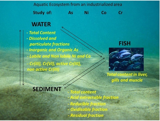
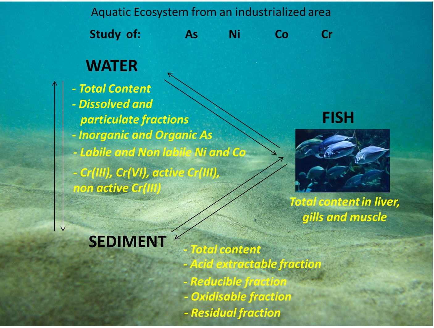
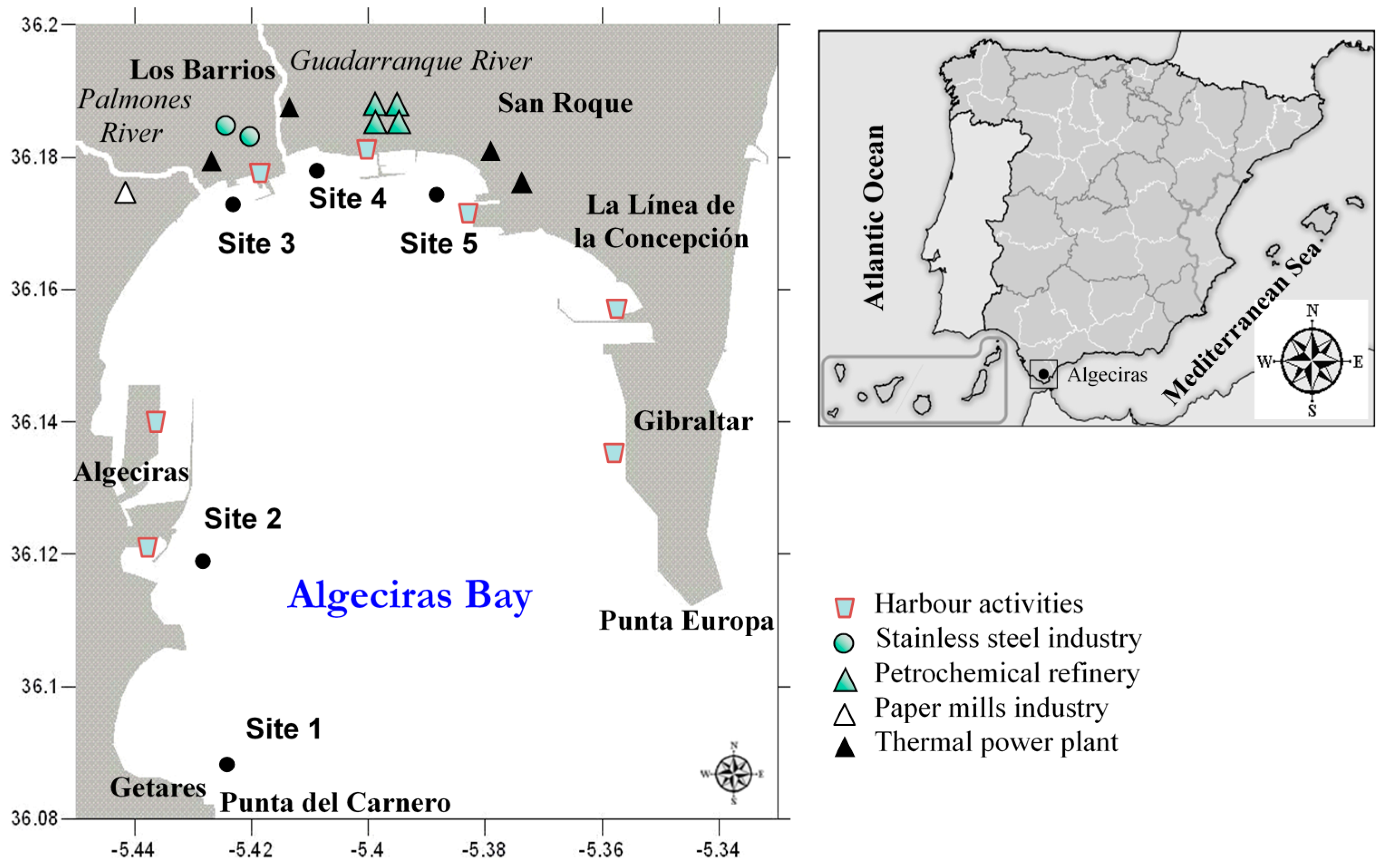
2.1. Description of the Study Area
2.2. Equipment
2.3. Physical-Chemical Parameters Analysis
2.4. Water Collection and Analysis
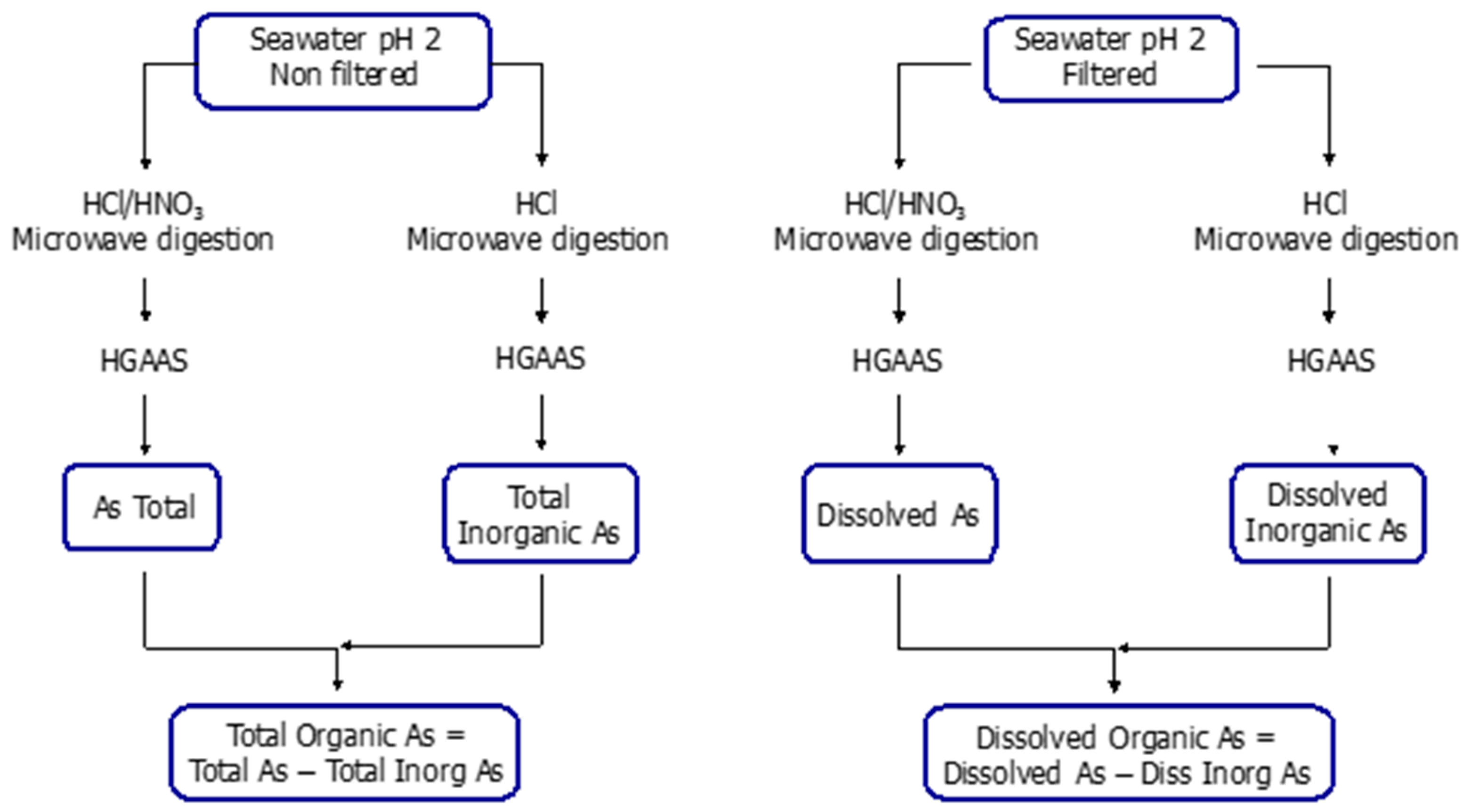
2.4.1. Arsenic Speciation
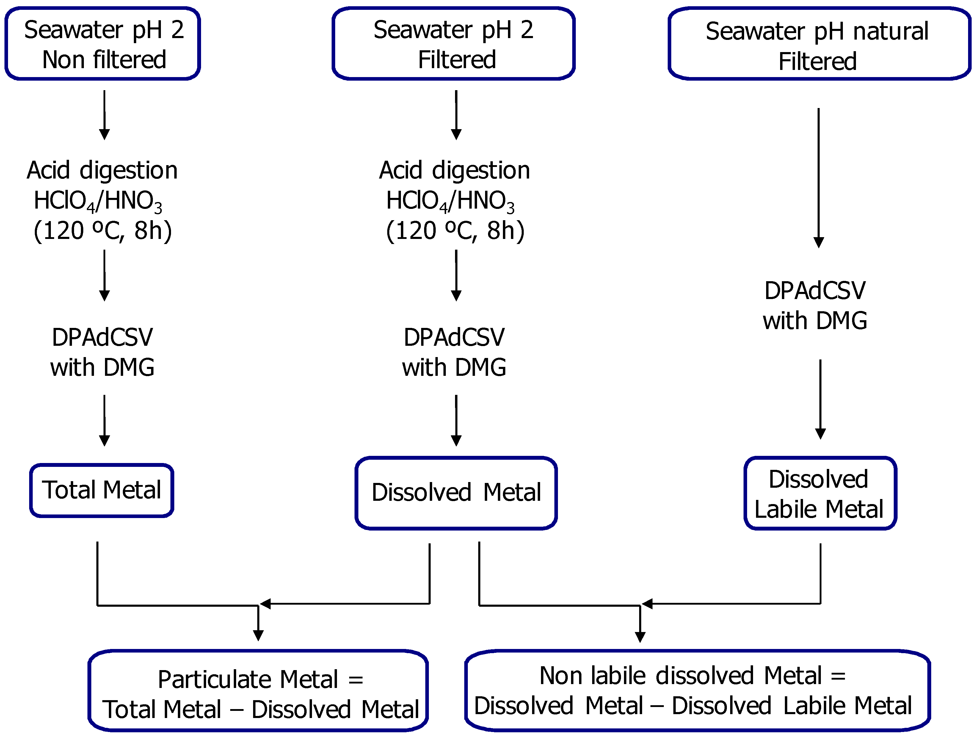
2.4.2. Nickel and Cobalt Speciation
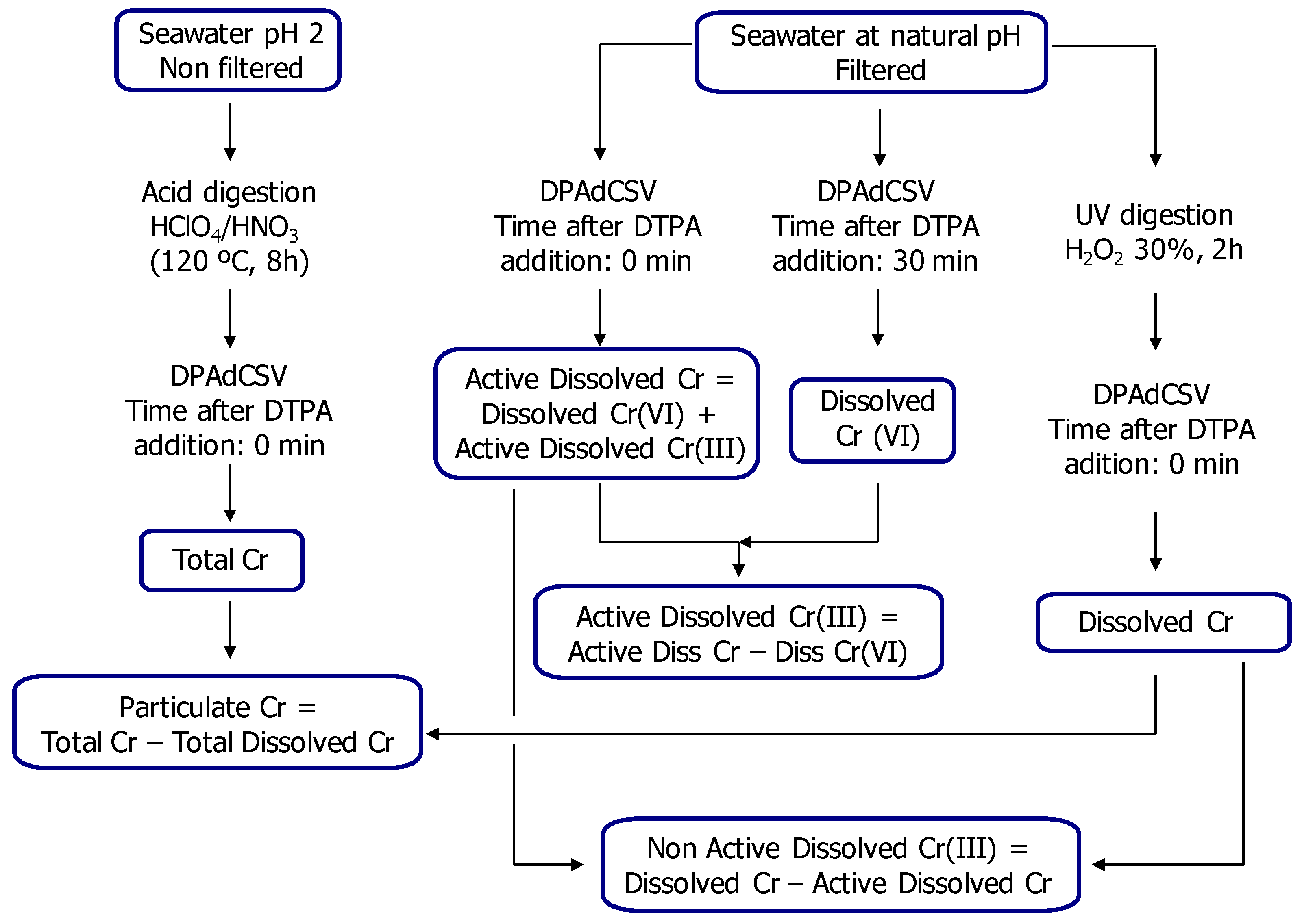
2.4.3. Chromium Speciation
2.5. Analysis of Collected Sediments
2.6. Analysis of Fish Collected
2.7. Quality Assurance and Quality Control (QA/QC)
2.8. Statistical Analyses
2.9. Pollution Indicators for the Assessment of Sediment Quality
3. Results and Discussion
3.1. Physical-Chemical Parameters
3.2. Metal and Semimetal Content in Water
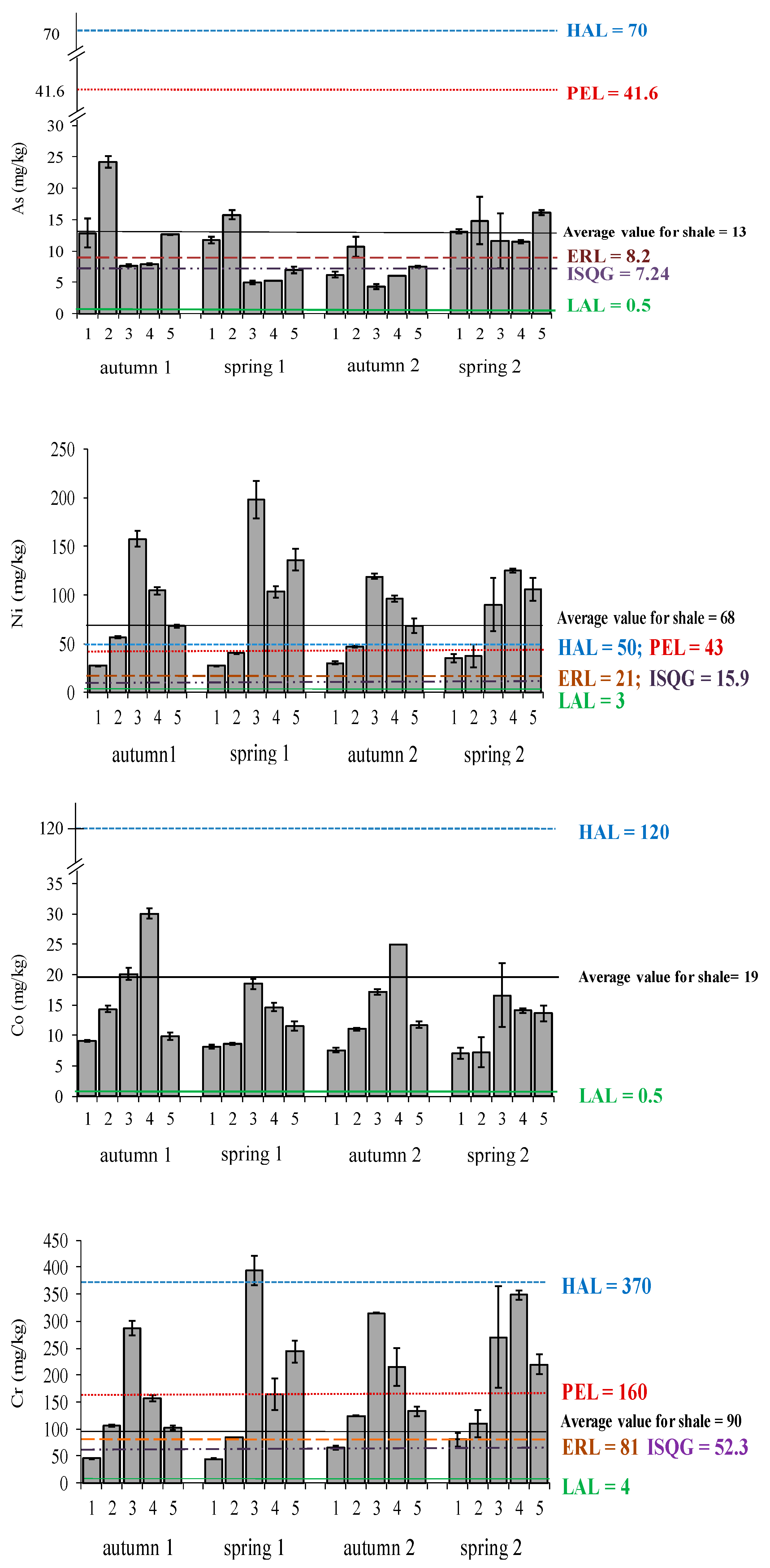
3.2.1. Total Metal and Semimetal Concentrations
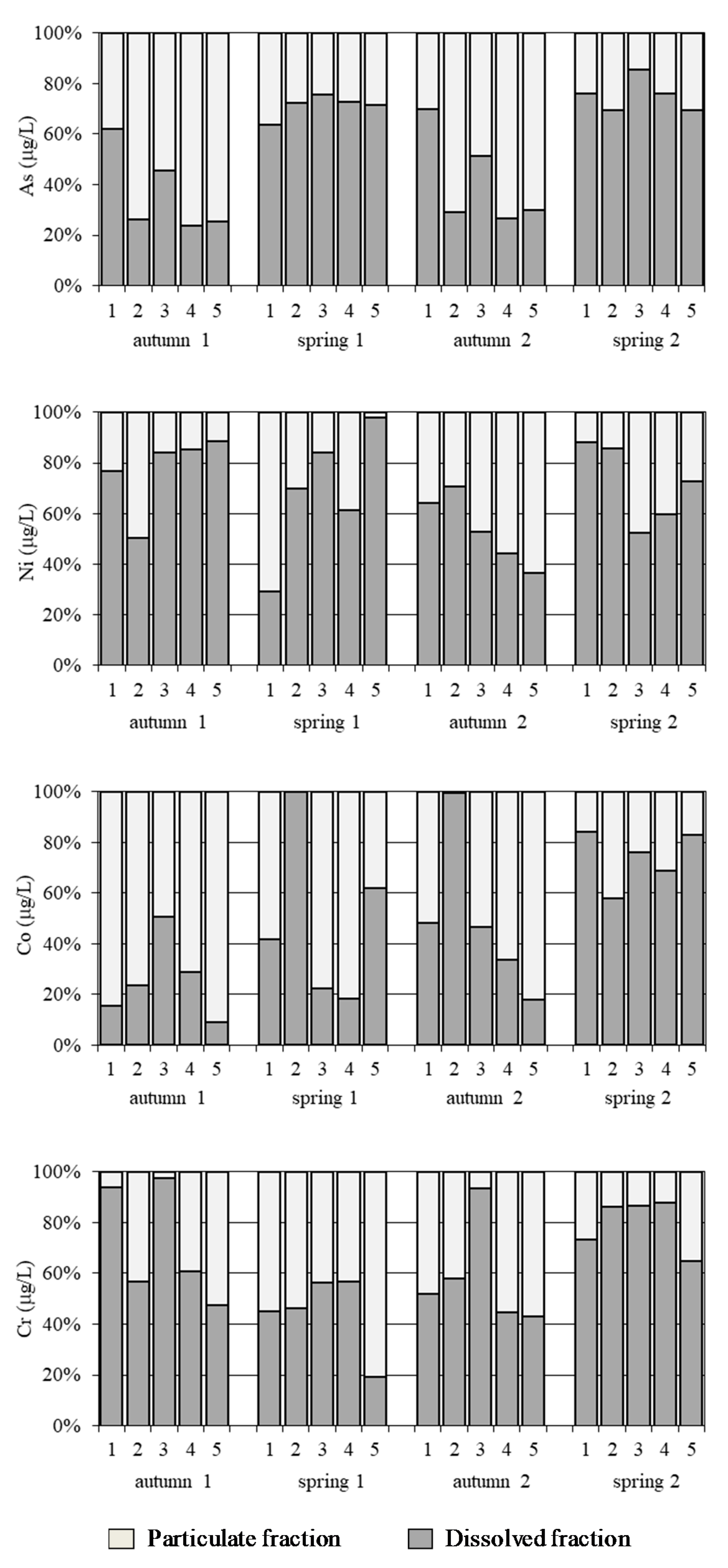
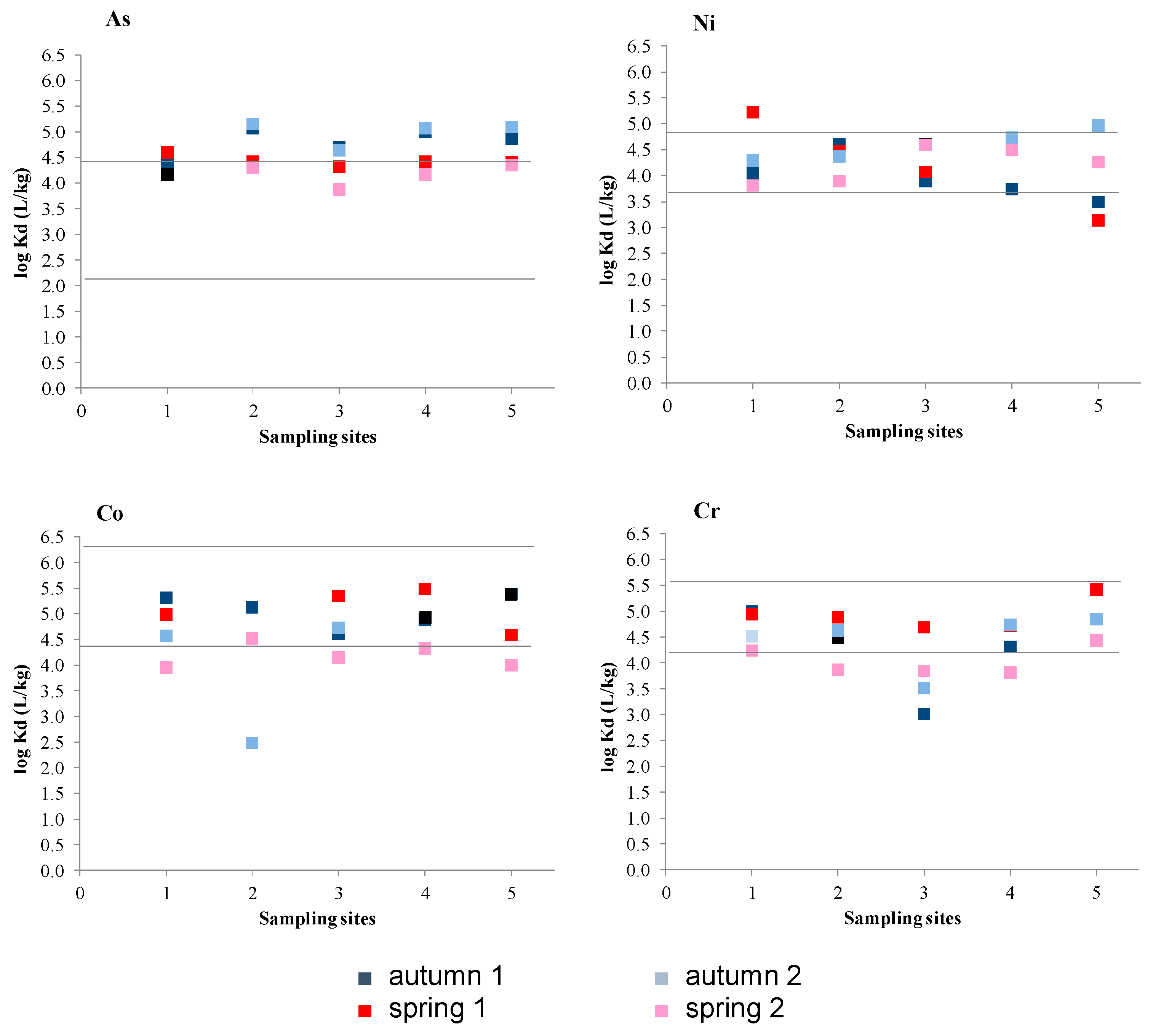
3.2.2. Distribution of Dissolved and Particulate Metals and Semimetals
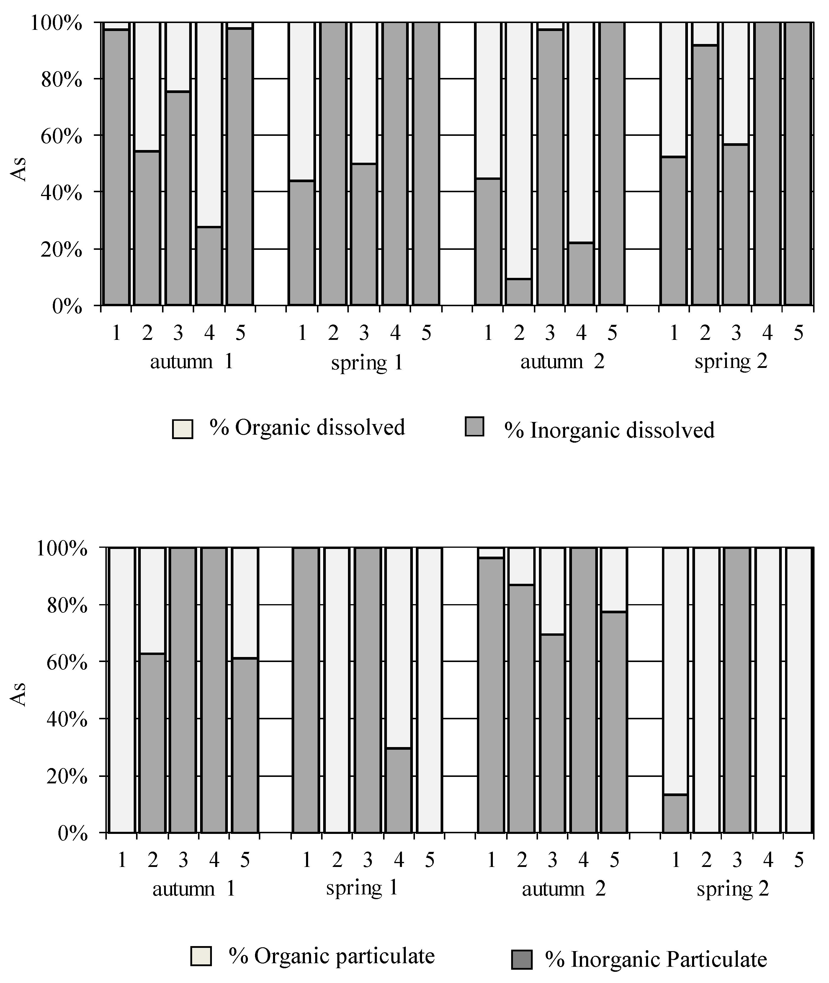
3.2.3. Arsenic (As) Speciation Data
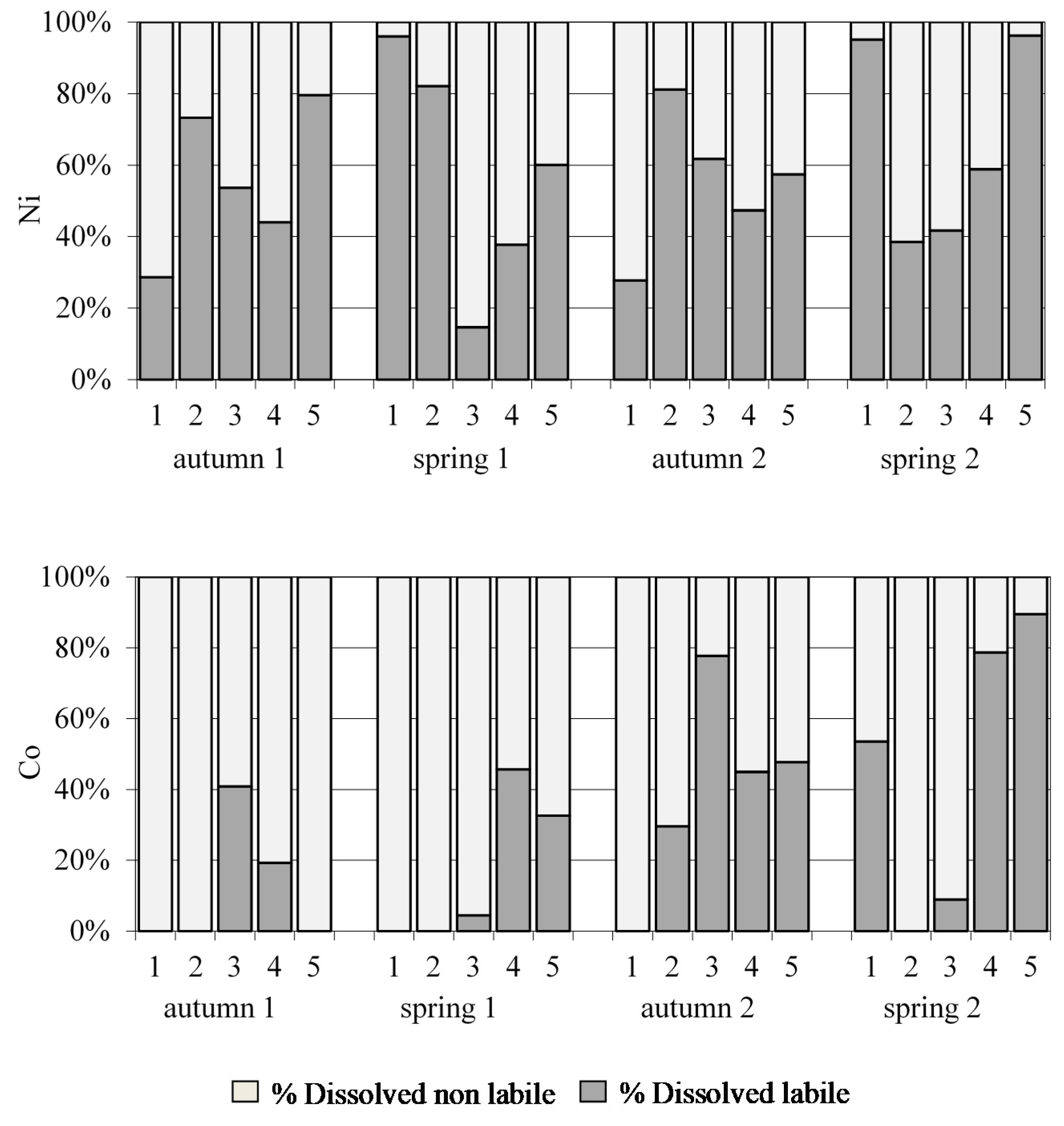
3.2.4. Cobalt (Co) and Nickel (Ni) Speciation Data
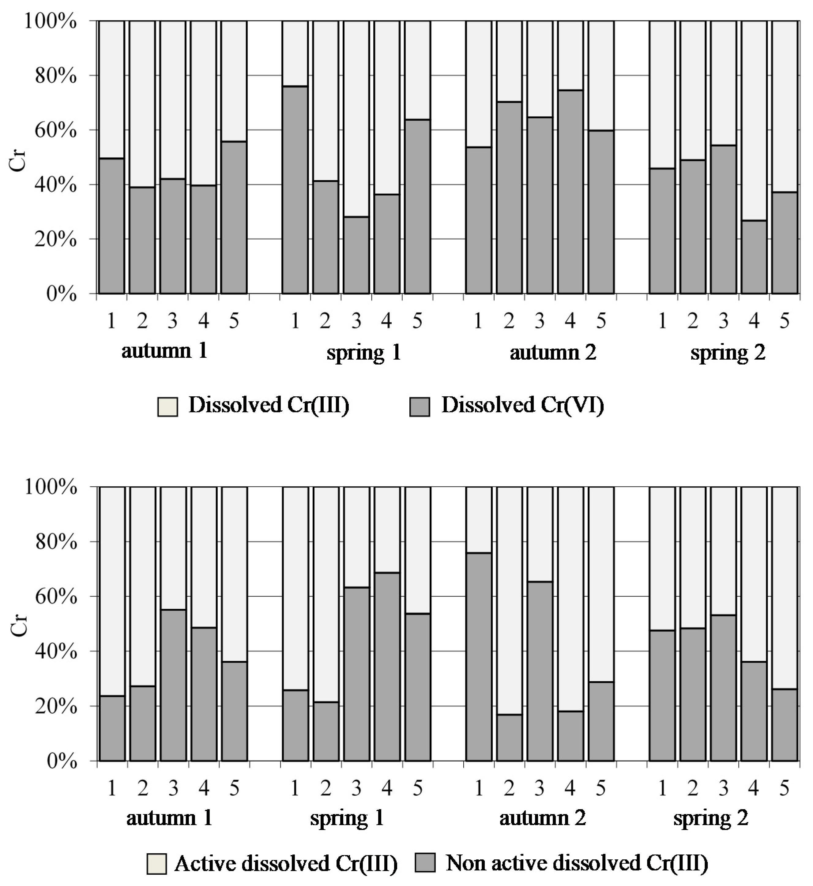
3.2.5. Chromium (Cr) Speciation Data
3.3. Metal and Semimetal Content in Sediments
3.3.1. Total Metal/Semimetal Concentrations
3.3.2. Speciation of Metals/Semimetals
3.4. Metal and Semimetal Content in Fish
3.5. Potential Hazardous Impacts of the Metals Studied in Algeciras Bay
3.6. Correlations among Water, Sediment and Fish
4. Conclusions
Author Contributions
Funding
Institutional Review Board Statement
Informed Consent Statement
Data Availability Statement
Acknowledgments
Conflicts of Interest
Appendix A

| Samplings | Sites | Sample | Species | Tissue | Length (cm) | Weight (g) | BFCW | BCFBS | ||||||
|---|---|---|---|---|---|---|---|---|---|---|---|---|---|---|
| As | Ni | Co | Cr | As | Ni | Co | Cr | |||||||
| Autumn 1 | 1 | 1 | Diplodus sargus sargus | L | 143 | 21 | 52 | 0.2 | 30.4 | 0.4 | 1.6 | 0.002 | 0.012 | 0.002 |
| Autumn 1 | 1 | 1 | Diplodus sargus sargus | G | 143 | 21 | 11 | 4.6 | 532.4 | 4.5 | 0.3 | 0.049 | 0.202 | 0.019 |
| Autumn 1 | 1 | 1 | Diplodus sargus sargus | M | 143 | 21 | 12 | 8.0 | 210.9 | 2.5 | 0.4 | 0.086 | 0.080 | 0.011 |
| Autumn 1 | 1 | 1 | Solea senegalensis | L | 236 | 29 | 36 | 0.4 | 53.9 | 1.5 | 1.1 | 0.004 | 0.020 | 0.006 |
| Autumn 1 | 1 | 1 | Solea senegalensis | M | 236 | 29 | 72 | n.d. | 20.9 | 1.4 | 2.2 | n.d. | 0.008 | 0.006 |
| Autumn 1 | 1 | 1 | Solea senegalensis | G | 236 | 29 | 11 | 1.6 | 79.9 | 7.9 | 0.3 | 0.017 | 0.030 | 0.033 |
| Autumn 1 | 1 | 2 | Solea senegalensis | L | 115 | 23 | 33 | 0.2 | 39.4 | 1.2 | 1.0 | 0.002 | 0.015 | 0.005 |
| Autumn 1 | 1 | 2 | Solea senegalensis | M | 115 | 23 | 38 | 0.4 | 10.1 | 2.7 | 1.2 | 0.005 | 0.004 | 0.011 |
| Autumn 1 | 1 | 2 | Solea senegalensis | G | 115 | 23 | 11 | 0.5 | 52.4 | 5.2 | 0.3 | 0.006 | 0.020 | 0.022 |
| Autumn 1 | 1 | 3 | Solea senegalensis | L | 225 | 28 | 53 | 0.1 | 28.4 | 0.6 | 1.6 | 0.002 | 0.011 | 0.003 |
| Autumn 1 | 1 | 3 | Solea senegalensis | G | 225 | 28 | 14 | 0.3 | 31.6 | 4.5 | 0.4 | 0.004 | 0.012 | 0.019 |
| Autumn 1 | 1 | 3 | Solea senegalensis | M | 225 | 28 | 52 | n.d. | 15.1 | 1.1 | 1.6 | n.d. | 0.006 | 0.005 |
| Autumn 1 | 3 | 1 | Trigloporus lastoviza | M | 355 | 32 | 18 | 0.4 | 2.3 | 1.7 | 0.6 | 0.001 | 0.006 | 0.002 |
| Autumn 1 | 3 | 1 | Trigloporus lastoviza | L | 355 | 32 | 10 | 0.5 | 20.2 | 0.1 | 0.3 | 0.001 | 0.050 | 0.000 |
| Autumn 1 | 5 | 2 | Trigloporus lastoviza | M | 76 | 20 | 103 | 0.4 | 33.3 | 2.1 | 1.5 | 0.001 | 0.014 | 0.003 |
| Autumn 1 | 5 | 2 | Trigloporus lastoviza | G | 76 | 20 | 85 | 0.5 | 48.5 | 1.2 | 1.2 | 0.002 | 0.020 | 0.002 |
| Autumn 1 | 5 | 2 | Trigloporus lastoviza | L | 76 | 20 | 112 | 2.6 | 184.3 | 1.4 | 1.6 | 0.008 | 0.075 | 0.002 |
| Autumn 1 | 5 | 4 | Solea senegalensis | M | 359 | 33 | 759 | 1.3 | 12.5 | 3.8 | 10.7 | 0.004 | 0.005 | 0.006 |
| Autumn 1 | 5 | 4 | Solea senegalensis | L | 359 | 33 | 2116 | 2.3 | 46.8 | 1.1 | 29.9 | 0.007 | 0.019 | 0.002 |
| Autumn 1 | 5 | 4 | Solea senegalensis | G | 359 | 33 | 150 | 3.5 | 61.8 | 7.8 | 2.1 | 0.011 | 0.025 | 0.012 |
| Spring 1 | 1 | 5 | Solea senegalensis | M | 135 | 24 | 88 | 1.5 | 3.8 | 1.9 | 3.5 | 0.006 | 0.006 | 0.006 |
| Spring 1 | 1 | 5 | Solea senegalensis | L | 135 | 24 | 33 | 1.6 | 20.3 | n.d. | 1.3 | 0.006 | 0.033 | n.d. |
| Spring 1 | 1 | 5 | Solea senegalensis | G | 135 | 24 | 11 | 4.0 | 17.1 | 2.6 | 0.4 | 0.016 | 0.028 | 0.008 |
| Spring 1 | 1 | 6 | Solea senegalensis | M | 136 | 24 | 99 | n.d. | 1.3 | 0.5 | 4.0 | n.d. | 0.002 | 0.002 |
| Spring 1 | 1 | 6 | Solea senegalensis | G | 136 | 24 | 16 | 2.9 | 12.1 | 7.3 | 0.7 | 0.011 | 0.020 | 0.022 |
| Spring 1 | 1 | 7 | Solea senegalensis | M | 114 | 21 | 56 | 1.5 | 3.0 | 1.8 | 2.2 | 0.006 | 0.005 | 0.006 |
| Spring 1 | 1 | 7 | Solea senegalensis | G | 114 | 21 | 15 | 15.8 | 14.4 | 7.5 | 0.6 | 0.062 | 0.024 | 0.023 |
| Spring 1 | 1 | 7 | Solea senegalensis | L | 114 | 21 | 477 | 129.7 | 204.1 | 122 | 19.3 | 0.507 | 0.335 | 0.372 |
| Spring 1 | 1 | 8 | Solea senegalensis | M | 170 | 26 | 104 | 0.0 | 3.2 | 0.8 | 4.2 | 0.000 | 0.005 | 0.002 |
| Spring 1 | 1 | 8 | Solea senegalensis | L | 170 | 26 | 39 | 0.8 | 31.3 | 0.5 | 1.6 | 0.003 | 0.051 | 0.001 |
| Spring 1 | 1 | 8 | Solea senegalensis | G | 170 | 26 | 12 | 3.5 | 14.4 | 5.2 | 0.5 | 0.014 | 0.024 | 0.016 |
| Spring 1 | 1 | 9 | Solea senegalensis | L | 149 | 25 | 200 | 3.1 | 40.0 | 1.4 | 8.1 | 0.012 | 0.066 | 0.004 |
| Spring 1 | 1 | 9 | Solea senegalensis | G | 149 | 25 | 18 | 1.8 | 20.1 | 3.1 | 0.7 | 0.007 | 0.033 | 0.010 |
| Spring 1 | 1 | 9 | Solea senegalensis | M | 149 | 25 | 179 | 2.4 | 2.2 | 0.3 | 7.2 | 0.009 | 0.004 | 0.001 |
| Spring 1 | 1 | 10 | Solea senegalensis | M | 153 | 26 | 126 | 1.9 | 2.9 | 2.7 | 5.1 | 0.008 | 0.005 | 0.008 |
| Spring 1 | 1 | 10 | Solea senegalensis | G | 153 | 26 | 15 | 10.2 | 18.1 | 12.5 | 0.6 | 0.040 | 0.030 | 0.038 |
| Spring 1 | 1 | 11 | Solea senegalensis | M | 183 | 28 | 123 | 0.7 | 3.1 | 1.7 | 5.0 | 0.003 | 0.005 | 0.005 |
| Spring 1 | 1 | 11 | Solea senegalensis | L | 183 | 28 | 148 | 1.1 | 33.1 | 0.9 | 6.0 | 0.004 | 0.054 | 0.003 |
| Spring 1 | 1 | 11 | Solea senegalensis | G | 183 | 28 | 19 | 2.2 | 20.9 | 4.9 | 0.8 | 0.009 | 0.034 | 0.015 |
| Spring 1 | 1 | 12 | Solea senegalensis | G | 112 | 23 | 10 | n.d. | 15.6 | 2.7 | 0.4 | n.d. | 0.026 | 0.008 |
| Spring 1 | 1 | 12 | Solea senegalensis | M | 112 | 23 | 52 | n.d. | 0.5 | 0.3 | 2.1 | n.d. | 0.001 | 0.001 |
| Spring 1 | 1 | 13 | Solea senegalensis | G | 130 | 25 | 9 | 8.3 | 10.9 | 15.2 | 0.4 | 0.032 | 0.018 | 0.047 |
| Spring 1 | 1 | 13 | Solea senegalensis | M | 130 | 25 | 74 | 0.8 | 1.8 | 2.8 | 3.0 | 0.003 | 0.003 | 0.008 |
| Spring 1 | 1 | 13 | Solea senegalensis | L | 130 | 25 | 25 | 1.1 | 8.6 | 0.1 | 1.0 | 0.004 | 0.014 | 0.000 |
| Spring 1 | 1 | 14 | Solea senegalensis | L | 134 | 24 | 34 | 0.3 | 14.1 | 0.4 | 1.4 | 0.001 | 0.023 | 0.001 |
| Spring 1 | 1 | 14 | Solea senegalensis | M | 134 | 24 | 84 | n.d. | 0.5 | 0.0 | 3.4 | n.d. | 0.001 | 0.000 |
| Spring 1 | 1 | 14 | Solea senegalensis | G | 134 | 24 | 14 | 0.9 | 17.0 | 3.3 | 0.6 | 0.004 | 0.028 | 0.010 |
| Spring 1 | 1 | 15 | Solea senegalensis | M | 274 | 31 | 153 | 2.2 | 2.3 | 1.2 | 6.2 | 0.009 | 0.004 | 0.004 |
| Spring 1 | 1 | 15 | Solea senegalensis | G | 274 | 31 | 19 | 9.2 | 34.0 | 5.0 | 0.7 | 0.036 | 0.056 | 0.015 |
| Spring 1 | 1 | 16 | Solea senegalensis | G | 199 | 28 | 8 | 2.8 | 9.6 | 4.7 | 0.3 | 0.011 | 0.016 | 0.014 |
| Spring 1 | 1 | 16 | Solea senegalensis | L | 199 | 28 | 35 | 0.7 | 16.1 | 0.6 | 1.4 | 0.003 | 0.026 | 0.002 |
| Spring 1 | 1 | 16 | Solea senegalensis | M | 199 | 28 | 65 | 0.4 | 1.9 | 2.7 | 2.6 | 0.002 | 0.003 | 0.008 |
| Spring 1 | 1 | 2 | Diplodus sargus sargus | M | 77 | 7.5 | 60 | n.d. | 0.9 | n.d. | 2.4 | n.d. | 0.001 | n.d. |
| Spring 1 | 1 | 2 | Diplodus sargus sargus | L | 77 | 7.5 | 40 | 1.7 | 45.3 | 0.5 | 1.6 | 0.007 | 0.074 | 0.001 |
| Spring 1 | 1 | 2 | Diplodus sargus sargus | G | 77 | 7.5 | 28 | 2.3 | 15.3 | 3.1 | 1.1 | 0.009 | 0.025 | 0.009 |
| Spring 1 | 1 | 17 | Solea senegalensis | M | 223 | 29 | 159 | 1.0 | 4.6 | 3.3 | 6.4 | 0.004 | 0.008 | 0.010 |
| Spring 1 | 1 | 17 | Solea senegalensis | L | 223 | 29 | 188 | 0.4 | 19.8 | 0.1 | 7.6 | 0.002 | 0.032 | 0.000 |
| Spring 1 | 1 | 17 | Solea senegalensis | G | 223 | 29 | 19 | 8.5 | 19.3 | 3.2 | 0.8 | 0.033 | 0.032 | 0.010 |
| Spring 1 | 1 | 18 | Solea senegalensis | G | 201 | 28 | 46 | 3.8 | 10.8 | 7.8 | 1.8 | 0.015 | 0.018 | 0.024 |
| Spring 1 | 1 | 18 | Solea senegalensis | M | 201 | 28 | 108 | 0.0 | 1.3 | 1.9 | 4.3 | 0.000 | 0.002 | 0.006 |
| Spring 1 | 1 | 18 | Solea senegalensis | L | 201 | 28 | 292 | 3.3 | 34.7 | 0.7 | 11.8 | 0.013 | 0.057 | 0.002 |
| Spring 1 | 2 | 19 | Solea senegalensis | L | 242 | 28 | 372 | 1.3 | 2.3 | 0.1 | 10.7 | 0.005 | 0.012 | 0.000 |
| Spring 1 | 2 | 19 | Solea senegalensis | M | 242 | 28 | 171 | n.d. | 0.3 | 0.1 | 4.9 | n.d. | 0.002 | 0.000 |
| Spring 1 | 2 | 19 | Solea senegalensis | G | 242 | 28 | 25 | 9.1 | 10.6 | 9.3 | 0.7 | 0.037 | 0.056 | 0.028 |
| Spring 1 | 2 | 20 | Solea senegalensis | M | 287 | 32 | 102 | 1.0 | 1.0 | 1.4 | 2.9 | 0.004 | 0.005 | 0.004 |
| Spring 1 | 2 | 20 | Solea senegalensis | G | 287 | 32 | 23 | 2.4 | 2.7 | 1.3 | 0.7 | 0.010 | 0.014 | 0.004 |
| Spring 1 | 2 | 21 | Solea senegalensis | M | 386 | 37 | 366 | n.d. | 0.4 | 0.4 | 10.5 | n.d. | 0.002 | 0.001 |
| Spring 1 | 2 | 21 | Solea senegalensis | G | 386 | 37 | 98 | 2.4 | 7.0 | 1.5 | 2.8 | 0.010 | 0.037 | 0.004 |
| Spring 1 | 3 | 22 | Solea senegalensis | G | 197 | 28 | 52 | 2.3 | 11.4 | 6.5 | 4.4 | 0.003 | 0.017 | 0.004 |
| Spring 1 | 3 | 22 | Solea senegalensis | L | 197 | 28 | 133 | 0.3 | 10.2 | 0.2 | 11.3 | 0.000 | 0.015 | 0.000 |
| Spring 1 | 3 | 22 | Solea senegalensis | M | 197 | 28 | 314 | n.d. | 0.1 | 0.1 | 26.6 | n.d. | 0.000 | 0.000 |
| Spring 1 | 3 | 3 | Trigloporus lastoviza | G | 339 | 35 | 17 | 1.5 | 16.5 | 1.1 | 1.4 | 0.002 | 0.024 | 0.001 |
| Spring 1 | 3 | 3 | Trigloporus lastoviza | L | 339 | 35 | 24 | 0.4 | 93.4 | 0.1 | 2.0 | 0.001 | 0.136 | 0.000 |
| Spring 1 | 3 | 3 | Trigloporus lastoviza | M | 339 | 35 | 22 | 1.9 | 2.2 | 0.4 | 1.9 | 0.002 | 0.003 | 0.000 |
| Spring 1 | 3 | 4 | Trigloporus lastoviza | L | 400 | 37 | 172 | 0.3 | 50.9 | 0.7 | 14.6 | 0.000 | 0.074 | 0.000 |
| Spring 1 | 3 | 4 | Trigloporus lastoviza | G | 400 | 37 | 89 | 1.6 | 18.4 | 1.3 | 7.5 | 0.002 | 0.027 | 0.001 |
| Spring 1 | 3 | 4 | Trigloporus lastoviza | M | 400 | 37 | 66 | n.d. | 4.4 | 0.2 | 5.6 | n.d. | 0.006 | 0.000 |
| Spring 1 | 3 | 5 | Trigloporus lastoviza | G | 371 | 34 | 91 | 2.8 | 28.7 | 4.9 | 7.7 | 0.003 | 0.042 | 0.003 |
| Spring 1 | 3 | 5 | Trigloporus lastoviza | M | 371 | 34 | 99 | n.d. | 5.7 | 0.7 | 8.4 | n.d. | 0.008 | 0.000 |
| Spring 1 | 3 | 5 | Trigloporus lastoviza | M | 371 | 38 | 199 | 0.4 | 128.8 | 0.1 | 16.9 | 0.001 | 0.188 | 0.000 |
| Spring 1 | 3 | 6 | Trigloporus lastoviza | L | 327 | 32 | 41 | 1.1 | 62.6 | 0.7 | 3.5 | 0.001 | 0.091 | 0.000 |
| Spring 1 | 3 | 6 | Trigloporus lastoviza | M | 327 | 32 | 72 | 0.1 | 6.1 | 0.4 | 6.1 | 0.000 | 0.009 | 0.000 |
| Spring 1 | 3 | 6 | Trigloporus lastoviza | G | 327 | 32 | 39 | 2.6 | 27.0 | 2.6 | 3.3 | 0.003 | 0.039 | 0.002 |
| Spring 1 | 3 | 7 | Trigloporus lastoviza | M | 353 | 34 | 13 | 0.1 | 2.9 | 0.2 | 1.1 | 0.000 | 0.004 | 0.000 |
| Spring 1 | 3 | 7 | Trigloporus lastoviza | G | 353 | 34 | 13 | 2.8 | 21.3 | 4.0 | 1.1 | 0.003 | 0.031 | 0.003 |
| Spring 1 | 3 | 7 | Trigloporus lastoviza | L | 353 | 32 | 15 | 1.9 | 168.5 | 0.0 | 1.3 | 0.002 | 0.246 | 0.000 |
| Spring 1 | 3 | 8 | Trigloporus lastoviza | L | 291 | 31 | 22 | 0.6 | 78.3 | 0.2 | 1.8 | 0.001 | 0.114 | 0.000 |
| Spring 1 | 3 | 8 | Trigloporus lastoviza | M | 291 | 31 | 29 | n.d. | 4.2 | 0.3 | 2.5 | n.d. | 0.006 | 0.000 |
| Spring 1 | 3 | 8 | Trigloporus lastoviza | G | 291 | 31 | 28 | 4.9 | 26.0 | 9.2 | 2.3 | 0.006 | 0.038 | 0.006 |
| Spring 1 | 3 | 9 | Trigloporus lastoviza | M | 319 | 34 | 82 | 0.1 | 2.1 | 0.4 | 6.9 | 0.000 | 0.003 | 0.000 |
| Spring 1 | 3 | 9 | Trigloporus lastoviza | L | 319 | 34 | 44 | 0.7 | 134.5 | 0.1 | 3.7 | 0.001 | 0.196 | 0.000 |
| Spring 1 | 3 | 9 | Trigloporus lastoviza | G | 319 | 34 | 42 | 2.2 | 19.6 | 2.3 | 3.5 | 0.003 | 0.029 | 0.002 |
| Spring 1 | 3 | 10 | Trigloporus lastoviza | M | 348 | 33 | 70 | n.d. | 2.3 | 0.2 | 5.9 | n.d. | 0.003 | 0.000 |
| Spring 1 | 3 | 10 | Trigloporus lastoviza | L | 348 | 33 | 51 | 0.1 | 42.4 | n.d. | 4.3 | 0.000 | 0.062 | n.d. |
| Spring 1 | 3 | 10 | Trigloporus lastoviza | G | 348 | 33 | 50 | 2.7 | 20.5 | 2.2 | 4.3 | 0.003 | 0.030 | 0.002 |
| Spring 1 | 3 | 11 | Trigloporus lastoviza | M | 400 | 39 | 62 | n.d. | 4.9 | 0.6 | 5.2 | n.d. | 0.007 | 0.000 |
| Spring 1 | 3 | 11 | Trigloporus lastoviza | L | 400 | 39 | 117 | 0.1 | 121.8 | 0.2 | 9.9 | 0.000 | 0.178 | 0.000 |
| Spring 1 | 3 | 11 | Trigloporus lastoviza | G | 400 | 39 | 48 | 3.4 | 29.9 | 3.1 | 4.1 | 0.004 | 0.044 | 0.002 |
| Spring 1 | 3 | 12 | Trigloporus lastoviza | L | 306 | 32 | 31 | 0.5 | 57.9 | 0.2 | 2.6 | 0.001 | 0.084 | 0.000 |
| Spring 1 | 3 | 12 | Trigloporus lastoviza | G | 306 | 32 | 25 | 1.8 | 22.9 | 3.5 | 2.1 | 0.002 | 0.033 | 0.002 |
| Spring 1 | 3 | 12 | Trigloporus lastoviza | M | 306 | 32 | 53 | n.d. | 5.3 | 0.9 | 4.5 | n.d. | 0.008 | 0.001 |
| Spring 1 | 3 | 13 | Trigloporus lastoviza | G | 290 | 38 | 34 | 4.1 | 35.4 | 6.6 | 2.9 | 0.005 | 0.052 | 0.005 |
| Spring 1 | 3 | 13 | Trigloporus lastoviza | L | 290 | 38 | 26 | 1.1 | 91.9 | 0.2 | 2.2 | 0.001 | 0.134 | 0.000 |
| Spring 1 | 3 | 13 | Trigloporus lastoviza | M | 290 | 38 | 34 | 1.0 | 4.0 | 0.2 | 2.8 | 0.001 | 0.006 | 0.000 |
| Spring 1 | 3 | 14 | Trigloporus lastoviza | M | 299 | 32 | 50 | n.d. | 2.9 | 0.3 | 4.2 | n.d. | 0.004 | 0.000 |
| Spring 1 | 3 | 14 | Trigloporus lastoviza | L | 299 | 32 | 57 | 0.7 | 69.1 | 0.3 | 4.8 | 0.001 | 0.101 | 0.000 |
| Spring 1 | 3 | 14 | Trigloporus lastoviza | G | 299 | 32 | 41 | 1.5 | 21.6 | 2.1 | 3.4 | 0.002 | 0.031 | 0.001 |
| Spring 1 | 4 | 23 | Solea senegalensis | M | 213 | 28 | 163 | 0.3 | 1.6 | 1.3 | 11.0 | 0.000 | 0.003 | 0.002 |
| Spring 1 | 4 | 23 | Solea senegalensis | L | 213 | 28 | 67 | 1.0 | 8.9 | 0.3 | 4.5 | 0.001 | 0.016 | 0.000 |
| Spring 1 | 4 | 23 | Solea senegalensis | G | 213 | 28 | 19 | 1.6 | 10.4 | 0.7 | 1.3 | 0.002 | 0.018 | 0.001 |
| Spring 1 | 5 | 24 | Solea senegalensis | G | 235 | 29 | 141 | 2.0 | 101.6 | 5.9 | 11.4 | 0.002 | 0.583 | 0.002 |
| Spring 1 | 5 | 24 | Solea senegalensis | L | 235 | 29 | 136 | 0.3 | 3.0 | 2.3 | 11.0 | 0.000 | 0.017 | 0.001 |
| Spring 1 | 5 | 24 | Solea senegalensis | M | 235 | 29 | 205 | n.d. | 0.3 | 1.8 | 16.6 | n.d. | 0.001 | 0.001 |
| Spring 1 | 5 | 25 | Solea senegalensis | L | 172 | 26 | 49 | n.d. | 3.7 | 0.6 | 4.0 | n.d. | 0.021 | 0.000 |
| Spring 1 | 5 | 25 | Solea senegalensis | G | 172 | 26 | 15 | 0.4 | 2.9 | 5.1 | 1.2 | 0.000 | 0.017 | 0.002 |
| Spring 1 | 5 | 25 | Solea senegalensis | M | 172 | 26 | 199 | 0.1 | 0.2 | 2.1 | 16.1 | 0.000 | 0.001 | 0.001 |
| Autumn 2 | 1 | 26 | Solea senegalensis | L | 174 | 25 | 44 | 1.1 | 8.1 | n.d. | 2.7 | 0.006 | 0.022 | n.d. |
| Autumn 2 | 1 | 26 | Solea senegalensis | G | 174 | 25 | 14 | 0.2 | 11.5 | 1.2 | 0.9 | 0.001 | 0.032 | 0.004 |
| Autumn 2 | 1 | 26 | Solea senegalensis | M | 174 | 25 | 90 | 0.2 | 3.7 | 0.7 | 5.6 | 0.001 | 0.010 | 0.002 |
| Autumn 2 | 1 | 27 | Solea senegalensis | L | 150 | 25 | 55 | 1.8 | 21.3 | 0.6 | 3.4 | 0.011 | 0.059 | 0.002 |
| Autumn 2 | 1 | 27 | Solea senegalensis | M | 150 | 25 | 88 | n.d. | 1.9 | 1.5 | 5.5 | n.d. | 0.005 | 0.005 |
| Autumn 2 | 1 | 28 | Solea senegalensis | L | 256 | 31 | 121 | 2.4 | 13.7 | n.d. | 7.6 | 0.014 | 0.038 | n.d. |
| Autumn 2 | 1 | 28 | Solea senegalensis | M | 256 | 31 | 194 | 0.4 | 0.9 | 0.3 | 12.1 | 0.002 | 0.002 | 0.001 |
| Autumn 2 | 1 | 28 | Solea senegalensis | G | 256 | 31 | 5 | 2.1 | 18.3 | 9.3 | 0.3 | 0.013 | 0.051 | 0.030 |
| Autumn 2 | 1 | 29 | Solea senegalensis | M | 237 | 29 | 97 | 2.3 | 3.2 | 2.4 | 6.0 | 0.014 | 0.009 | 0.008 |
| Autumn 2 | 1 | 29 | Solea senegalensis | G | 237 | 29 | 11 | 4.2 | 11.0 | 0.2 | 0.7 | 0.025 | 0.031 | 0.001 |
| Autumn 2 | 1 | 1 | Scorpaena porcus | L | >440 | 50 | 54 | 1.4 | 18.4 | 0.2 | 3.4 | 0.008 | 0.051 | 0.001 |
| Autumn 2 | 1 | 30 | Solea senegalensis | M | 223 | 29 | 122 | 0.1 | 4.5 | 1.1 | 7.6 | 0.000 | 0.012 | 0.003 |
| Autumn 2 | 1 | 30 | Solea senegalensis | G | 223 | 29 | 12 | 0.4 | 15.0 | 2.6 | 0.7 | 0.002 | 0.042 | 0.009 |
| Autumn 2 | 1 | 2 | Scorpaena porcus | L | 345 | 26 | 34 | 0.7 | 69.5 | n.d. | 2.2 | 0.004 | 0.193 | n.d. |
| Autumn 2 | 1 | 2 | Scorpaena porcus | G | 345 | 26 | 7 | 2.6 | 19.3 | 1.5 | 0.4 | 0.016 | 0.054 | 0.005 |
| Autumn 2 | 1 | 2 | Scorpaena porcus | G | 345 | 26 | 13 | 2.7 | 17.3 | 3.4 | 0.8 | 0.016 | 0.048 | 0.011 |
| Autumn 2 | 1 | 2 | Scorpaena porcus | M | 345 | 26 | 21 | n.d. | 2.2 | 2.5 | 1.3 | n.d. | 0.006 | 0.008 |
| Autumn 2 | 1 | 15 | Trigloporus lastoviza | G | 261 | 29 | 8 | 0.0 | 12.2 | n.d. | 0.5 | 0.000 | 0.034 | n.d. |
| Autumn 2 | 1 | 15 | Trigloporus lastoviza | L | 261 | 29 | 27 | 1.2 | 35.8 | 0.0 | 1.7 | 0.007 | 0.099 | 0.000 |
| Autumn 2 | 1 | 3 | Scorpaena porcus | L | 206 | 20 | 11 | 0.1 | 12.7 | n.d. | 0.7 | 0.000 | 0.035 | n.d. |
| Autumn 2 | 1 | 3 | Scorpaena porcus | G | 206 | 20 | 7 | 1.7 | 15.0 | 0.5 | 0.4 | 0.010 | 0.042 | 0.002 |
| Autumn 2 | 1 | 3 | Scorpaena porcus | M | 206 | 20 | 43 | n.d. | 2.5 | 0.1 | 2.7 | n.d. | 0.007 | 0.000 |
| Autumn 2 | 1 | 31 | Solea senegalensis | L | 348 | 35 | 67 | 2.5 | 11.2 | 0.0 | 4.2 | 0.015 | 0.031 | 0.000 |
| Autumn 2 | 1 | 31 | Solea senegalensis | G | 348 | 35 | 5 | 0.3 | 9.5 | 0.9 | 0.3 | 0.002 | 0.026 | 0.003 |
| Autumn 2 | 1 | 31 | Solea senegalensis | M | 348 | 35 | 118 | n.d. | 0.3 | 0.5 | 7.4 | n.d. | 0.001 | 0.001 |
| Autumn 2 | 1 | 4 | Scorpaena porcus | L | 324 | 25 | 14 | 0.1 | 16.4 | n.d. | 0.9 | 0.001 | 0.045 | n.d. |
| Autumn 2 | 1 | 4 | Scorpaena porcus | G | 324 | 25 | 9 | 1.0 | 15.5 | 0.2 | 0.6 | 0.006 | 0.043 | 0.001 |
| Autumn 2 | 1 | 4 | Scorpaena porcus | M | 324 | 25 | 19 | 0.2 | 5.0 | 3.3 | 1.2 | 0.001 | 0.014 | 0.011 |
| Autumn 2 | 1 | 4 | Scorpaena porcus | M | 324 | 25 | 19 | 1.0 | 2.5 | 1.6 | 1.2 | 0.006 | 0.007 | 0.005 |
| Autumn 2 | 1 | 5 | Scorpaena porcus | M | >440 | 34 | 10 | 0.4 | 6.2 | 1.1 | 0.6 | 0.002 | 0.017 | 0.004 |
| Autumn 2 | 1 | 5 | Scorpaena porcus | M | >440 | 34 | 17 | 0.1 | 2.9 | 0.5 | 1.1 | 0.001 | 0.008 | 0.002 |
| Autumn 2 | 1 | 5 | Scorpaena porcus | G | >440 | 34 | 7 | 1.1 | 10.2 | 0.4 | 0.5 | 0.006 | 0.028 | 0.001 |
| Autumn 2 | 2 | 6 | Scorpaena porcus | L | >440 | 31 | 44 | 0.2 | 21.2 | n.d. | 0.7 | 0.001 | 0.066 | n.d. |
| Autumn 2 | 2 | 6 | Scorpaena porcus | M | >440 | 31 | 42 | n.d. | 2.0 | 1.6 | 0.7 | n.d. | 0.006 | 0.003 |
| Autumn 2 | 2 | 6 | Scorpaena porcus | G | >440 | 31 | 35 | 0.7 | 9.2 | 1.4 | 0.6 | 0.001 | 0.028 | 0.003 |
| Autumn 2 | 2 | 7 | Scorpaena porcus | L | 284 | 28 | 32 | 2.1 | 33.5 | n.d. | 0.5 | 0.004 | 0.104 | n.d. |
| Autumn 2 | 2 | 7 | Scorpaena porcus | M | 234 | 28 | 94 | 1.1 | 7.6 | 1.0 | 1.6 | 0.002 | 0.024 | 0.002 |
| Autumn 2 | 2 | 7 | Scorpaena porcus | G | 234 | 28 | 50 | 4.4 | 21.1 | 0.9 | 0.8 | 0.009 | 0.065 | 0.002 |
| Autumn 2 | 2 | 8 | Scorpaena porcus | M | 341 | 26 | 69 | n.d. | 3.0 | 0.6 | 1.2 | n.d. | 0.009 | 0.001 |
| Autumn 2 | 2 | 8 | Scorpaena porcus | L | 293 | 24 | 19 | 0.5 | 20.1 | n.d. | 0.3 | 0.001 | 0.062 | n.d. |
| Autumn 2 | 2 | 8 | Scorpaena porcus | G | 293 | 24 | 19 | 3.8 | 12.8 | 0.7 | 0.3 | 0.008 | 0.039 | 0.001 |
| Autumn 2 | 2 | 9 | Scorpaena porcus | L | 341 | 28 | 61 | 1.3 | 118.8 | 0.2 | 1.0 | 0.003 | 0.367 | 0.000 |
| Autumn 2 | 2 | 9 | Scorpaena porcus | G | 341 | 26 | 49 | 1.5 | 3.4 | 0.0 | 0.8 | 0.003 | 0.011 | 0.000 |
| Autumn 2 | 3 | 16 | Trigloporus lastoviza | M | 175 | 26 | 39 | 0.1 | 1.7 | 0.6 | 2.3 | 0.000 | 0.007 | 0.000 |
| Autumn 2 | 3 | 16 | Trigloporus lastoviza | G | 175 | 26 | 24 | 2.4 | 5.4 | 1.4 | 1.4 | 0.005 | 0.023 | 0.001 |
| Autumn 2 | 3 | 32 | Solea senegalensis | L | 196 | 26 | 58 | 0.6 | 2.4 | 0.1 | 3.4 | 0.001 | 0.010 | 0.000 |
| Autumn 2 | 3 | 32 | Solea senegalensis | M | 196 | 26 | 143 | 0.1 | 1.0 | 0.4 | 8.5 | 0.000 | 0.004 | 0.000 |
| Autumn 2 | 3 | 33 | Solea senegalensis | L | 745 | 20 | 36 | 1.9 | 3.1 | 1.0 | 2.2 | 0.004 | 0.013 | 0.001 |
| Autumn 2 | 3 | 33 | Solea senegalensis | G | 75 | 20 | 8 | 2.0 | 4.6 | 9.1 | 0.5 | 0.004 | 0.019 | 0.008 |
| Autumn 2 | 3 | 33 | Solea senegalensis | M | 75 | 20 | 37 | 0.0 | 0.3 | 0.9 | 2.2 | 0.000 | 0.001 | 0.001 |
| Autumn 2 | 3 | 17 | Trigloporus lastoviza | L | 177 | 27 | 45 | 1.4 | 49.9 | n.d. | 2.7 | 0.003 | 0.209 | n.d. |
| Autumn 2 | 3 | 17 | Trigloporus lastoviza | G | 177 | 27 | n.d. | n.d. | n.d. | n.d. | n.d. | n.d. | n.d. | n.d. |
| Autumn 2 | 3 | 17 | Trigloporus lastoviza | M | 177 | 27 | 63 | n.d. | 0.8 | 0.6 | 3.8 | n.d. | 0.003 | 0.001 |
| Autumn 2 | 3 | 34 | Solea senegalensis | L | 148 | 26 | 112 | 2.7 | 8.8 | 2.8 | 6.6 | 0.006 | 0.037 | 0.002 |
| Autumn 2 | 3 | 34 | Solea senegalensis | G | 148 | 26 | 20 | 3.6 | 3.5 | 0.7 | 1.2 | 0.008 | 0.015 | 0.001 |
| Autumn 2 | 3 | 34 | Solea senegalensis | M | 148 | 26 | 88 | 0.1 | 0.6 | 1.5 | 5.2 | 0.000 | 0.003 | 0.001 |
| Autumn 2 | 3 | 34 | Solea senegalensis | M | 217 | 30 | n.d. | n.d. | n.d. | n.d. | n.d. | n.d. | n.d. | n.d. |
| Autumn 2 | 3 | 35 | Solea senegalensis | G | 217 | 30 | 19 | 0.7 | 4.0 | 2.5 | 1.1 | 0.002 | 0.017 | 0.002 |
| Autumn 2 | 3 | 35 | Solea senegalensis | L | 217 | 30 | 65 | 2.7 | 23.7 | n.d. | 3.9 | 0.006 | 0.099 | n.d. |
| Autumn 2 | 4 | 18 | Trigloporus lastoviza | M | 175 | 26 | 107 | n.d. | 0.4 | 8.3 | 2.9 | n.d. | 0.004 | 0.009 |
| Autumn 2 | 4 | 18 | Trigloporus lastoviza | L | 175 | 26 | 181 | 6.0 | 40.7 | 0.5 | 4.8 | 0.015 | 0.413 | 0.001 |
| Autumn 2 | 4 | 18 | Trigloporus lastoviza | G | 175 | 26 | 82 | 1.0 | 3.3 | 0.7 | 2.2 | 0.002 | 0.034 | 0.001 |
| Autumn 2 | 4 | 10 | Scorpaena porcus | L | 108 | 18 | 23 | 0.6 | 1.5 | 0.1 | 0.6 | 0.002 | 0.016 | 0.000 |
| Autumn 2 | 4 | 10 | Scorpaena porcus | G | 133 | 19 | 22 | 2.0 | 2.3 | 0.8 | 0.6 | 0.005 | 0.024 | 0.001 |
| Autumn 2 | 4 | 10 | Scorpaena porcus | M | 133 | 19 | 263 | n.d. | 0.7 | 0.6 | 7.0 | n.d. | 0.007 | 0.001 |
| Autumn 2 | 4 | 11 | Scorpaena porcus | M | 108 | 18 | 228 | n.d. | 0.6 | 1.1 | 6.1 | n.d. | 0.006 | 0.001 |
| Autumn 2 | 4 | 11 | Scorpaena porcus | G | 108 | 18 | 22 | 0.8 | 2.3 | 1.3 | 0.6 | 0.002 | 0.024 | 0.001 |
| Autumn 2 | 4 | 19 | Trigloporus lastoviza | M | 135 | 23 | 83 | n.d. | 0.5 | 1.8 | 2.2 | n.d. | 0.005 | 0.002 |
| Autumn 2 | 4 | 19 | Trigloporus lastoviza | L | 135 | 23 | 102 | 1.0 | 17.1 | n.d. | 2.7 | 0.002 | 0.174 | n.d. |
| Autumn 2 | 4 | 19 | Trigloporus lastoviza | G | 135 | 23 | 77 | 1.5 | 4.3 | 2.1 | 2.1 | 0.004 | 0.044 | 0.002 |
| Autumn 2 | 4 | 20 | Trigloporus lastoviza | M | 135 | 24 | 144 | n.d. | 0.8 | 0.4 | 3.8 | n.d. | 0.009 | 0.000 |
| Autumn 2 | 4 | 20 | Trigloporus lastoviza | G | 135 | 24 | 62 | 0.9 | 6.6 | 0.0 | 1.7 | 0.002 | 0.067 | 0.000 |
| Autumn 2 | 4 | 20 | Trigloporus lastoviza | L | 135 | 23 | 88 | 2.2 | 0.5 | n.d. | 2.3 | 0.005 | 0.005 | n.d. |
| Autumn 2 | 5 | 21 | Trigloporus lastoviza | L | 124 | 23 | 257 | 6.6 | 1003.3 | 0.5 | 7.2 | 0.007 | 0.943 | 0.001 |
| Autumn 2 | 5 | 21 | Trigloporus lastoviza | G | 124 | 23 | 67 | 3.9 | 124.1 | 1.0 | 1.9 | 0.004 | 0.117 | 0.002 |
| Autumn 2 | 5 | 37 | Solea senegalensis | G | >440 | 36 | 9 | 2.7 | 25.7 | 0.4 | 0.2 | 0.003 | 0.024 | 0.001 |
| Autumn 2 | 5 | 36 | Solea senegalensis | M | >440 | 36 | 97 | 1.0 | 2.1 | 0.8 | 2.7 | 0.001 | 0.002 | 0.001 |
| Autumn 2 | 5 | 36 | Solea senegalensis | L | >440 | 36 | 90 | 4.2 | 11.2 | 0.2 | 2.5 | 0.004 | 0.011 | 0.000 |
| Autumn 2 | 5 | 37 | Solea senegalensis | M | 43 | 35 | 392 | n.d. | 2.4 | 3.0 | 11.0 | n.d. | 0.002 | 0.005 |
| Autumn 2 | 5 | 37 | Solea senegalensis | G | 43 | 35 | 40 | 9.1 | 39.3 | 5.2 | 1.1 | 0.010 | 0.037 | 0.008 |
| Autumn 2 | 5 | 37 | Solea senegalensis | L | 43 | 35 | 25 | 1.0 | 71.2 | 0.2 | 0.7 | 0.001 | 0.067 | 0.000 |
| Autumn 2 | 5 | 38 | Solea senegalensis | M | 137 | 28 | 148 | 7.8 | 2.5 | 0.5 | 4.2 | 0.008 | 0.002 | 0.001 |
| Autumn 2 | 5 | 38 | Solea senegalensis | G | 137 | 28 | 30 | 6.6 | 22.4 | 2.7 | 0.8 | 0.007 | 0.021 | 0.004 |
| Spring 2 | 1 | 39 | Solea senegalensis | G | 193 | 26 | 7 | 3.9 | 2.4 | 1.1 | 0.3 | 0.018 | 0.009 | 0.003 |
| Spring 2 | 1 | 39 | Solea senegalensis | M | 193 | 26 | 64 | 1.4 | 0.6 | 2.5 | 2.7 | 0.007 | 0.002 | 0.007 |
| Spring 2 | 1 | 39 | Solea senegalensis | L | 193 | 26 | 15 | 0.3 | 2.8 | 0.4 | 0.6 | 0.001 | 0.010 | 0.001 |
| Spring 2 | 1 | 40 | Solea senegalensis | M | 193 | 26 | 115 | 2.4 | 1.2 | 1.4 | 4.9 | 0.011 | 0.004 | 0.004 |
| Spring 2 | 1 | 40 | Solea senegalensis | G | 193 | 26 | 10 | 4.9 | 5.4 | 1.9 | 0.4 | 0.023 | 0.019 | 0.006 |
| Spring 2 | 1 | 40 | Solea senegalensis | L | 193 | 26 | 42 | 0.8 | 5.8 | 0.2 | 1.8 | 0.004 | 0.021 | 0.001 |
| Spring 2 | 1 | 41 | Solea senegalensis | G | 130 | 24 | 9 | 5.1 | 2.5 | 2.2 | 0.4 | 0.024 | 0.009 | 0.006 |
| Spring 2 | 1 | 41 | Solea senegalensis | L | 130 | 24 | 27 | 2.6 | 5.0 | 2.1 | 1.1 | 0.012 | 0.018 | 0.006 |
| Spring 2 | 1 | 41 | Solea senegalensis | M | 130 | 24 | 91 | 0.7 | 0.3 | 1.7 | 3.9 | 0.003 | 0.001 | 0.005 |
| Spring 2 | 1 | 42 | Solea senegalensis | M | 122 | 25 | 111 | 0.8 | 0.5 | 0.4 | 4.7 | 0.004 | 0.002 | 0.001 |
| Spring 2 | 1 | 42 | Solea senegalensis | L | 122 | 25 | 19 | 1.9 | 2.8 | 0.7 | 0.8 | 0.009 | 0.010 | 0.002 |
| Spring 2 | 1 | 42 | Solea senegalensis | G | 122 | 25 | 8 | 3.1 | 1.6 | 10.6 | 0.3 | 0.015 | 0.005 | 0.031 |
| Spring 2 | 1 | 43 | Solea senegalensis | G | 166 | 26 | 4 | 11.0 | 4.3 | 4.8 | 0.2 | 0.052 | 0.015 | 0.014 |
| Spring 2 | 1 | 43 | Solea senegalensis | M | 166 | 26 | 68 | 1.7 | 0.7 | 2.5 | 2.9 | 0.008 | 0.003 | 0.007 |
| Spring 2 | 1 | 43 | Solea senegalensis | L | 166 | 26 | 26 | 0.7 | 5.5 | n.d. | 1.1 | 0.003 | 0.019 | n.d. |
| Spring 2 | 1 | 44 | Solea senegalensis | G | 117 | 23 | 1 | 0.8 | 0.6 | 0.8 | 0.0 | 0.004 | 0.002 | 0.002 |
| Spring 2 | 1 | 44 | Solea senegalensis | M | 117 | 23 | 87 | 1.1 | 0.4 | 0.7 | 3.7 | 0.005 | 0.002 | 0.002 |
| Spring 2 | 1 | 44 | Solea senegalensis | L | 117 | 23 | 46 | 1.5 | 55.8 | 2.4 | 1.7 | 0.007 | 0.194 | 0.005 |
| Spring 2 | 1 | 45 | Solea senegalensis | M | 82 | 20 | 62 | 1.9 | 1.0 | 1.6 | 2.6 | 0.009 | 0.004 | 0.005 |
| Spring 2 | 1 | 45 | Solea senegalensis | G | 82 | 20 | 6 | 9.9 | 5.9 | 11.1 | 0.3 | 0.046 | 0.021 | 0.033 |
| Spring 2 | 1 | 45 | Solea senegalensis | L | 82 | 20 | 2 | 0.3 | 1.6 | 0.0 | 0.1 | 0.000 | 0.003 | 0.000 |
| Spring 2 | 1 | 12 | Scorpaena porcus | M | 149 | 20 | 21 | 1.6 | 1.0 | 1.8 | 0.9 | 0.007 | 0.004 | 0.005 |
| Spring 2 | 1 | 12 | Scorpaena porcus | G | 149 | 20 | 7 | 2.9 | 5.4 | 1.5 | 0.3 | 0.014 | 0.019 | 0.004 |
| Spring 2 | 1 | 12 | Scorpaena porcus | L | 149 | 20 | 22 | 0.3 | 23.0 | 0.3 | 0.9 | 0.001 | 0.081 | 0.001 |
| Spring 2 | 1 | 3 | Diplodus sargus sargus | G | 149 | 20 | 11 | 1.5 | 4.7 | 1.8 | 0.4 | 0.007 | 0.017 | 0.005 |
| Spring 2 | 1 | 3 | Diplodus sargus sargus | M | 149 | 20 | 10 | 2.0 | 0.4 | 1.2 | 0.4 | 0.010 | 0.001 | 0.003 |
| Spring 2 | 1 | 3 | Diplodus sargus sargus | L | 149 | 20 | 20 | 2.1 | 28.1 | n.d. | 0.9 | 0.010 | 0.099 | n.d. |
| Spring 2 | 2 | 4 | Diplodus sargus sargus | L | 60 | 36 | 50 | 3.4 | 115.9 | 0.3 | 1.8 | 0.020 | 0.278 | 0.001 |
| Spring 2 | 2 | 4 | Diplodus sargus sargus | M | 60 | 36 | 64 | 1.5 | 4.1 | 0.7 | 2.0 | 0.009 | 0.010 | 0.002 |
| Spring 2 | 2 | 4 | Diplodus sargus sargus | G | 60 | 36 | 23 | 3.1 | 25.7 | 1.2 | 0.7 | 0.018 | 0.061 | 0.004 |
| Spring 2 | 2 | 5 | Diplodus sargus sargus | M | 153 | 21 | 54 | 1.1 | 3.4 | 0.7 | 1.7 | 0.006 | 0.008 | 0.002 |
| Spring 2 | 2 | 5 | Diplodus sargus sargus | G | 153 | 21 | 23 | 2.5 | 17.4 | 1.8 | 0.7 | 0.014 | 0.041 | 0.006 |
| Spring 2 | 2 | 5 | Diplodus sargus sargus | L | 153 | 21 | 18 | 1.4 | 43.2 | 0.1 | 0.6 | 0.008 | 0.102 | 0.000 |
| Spring 2 | 4 | 46 | Solea senegalensis | G | 202 | 27 | 9 | 3.3 | 3.6 | 5.0 | 0.3 | 0.009 | 0.009 | 0.005 |
| Spring 2 | 4 | 46 | Solea senegalensis | M | 202 | 27 | 112 | 1.2 | 0.5 | 1.4 | 4.2 | 0.003 | 0.001 | 0.001 |
| Spring 2 | 4 | 46 | Solea senegalensis | L | 202 | 27 | 38 | 0.1 | 5.7 | 0.1 | 1.4 | 0.000 | 0.015 | 0.000 |
| Spring 2 | 4 | 47 | Solea senegalensis | G | 79 | 20 | 47 | 7.8 | 3.5 | 2.6 | 1.7 | 0.021 | 0.009 | 0.003 |
| Spring 2 | 4 | 47 | Solea senegalensis | L | 79 | 20 | 22 | 0.1 | 1.1 | n.d. | 0.8 | 0.000 | 0.003 | n.d. |
| Spring 2 | 4 | 22 | Trigloporus lastoviza | L | 113 | 22 | 21 | 1.4 | 171.5 | 0.1 | 0.7 | 0.014 | 0.894 | 0.000 |
| Spring 2 | 4 | 22 | Trigloporus lastoviza | G | 113 | 22 | 15 | 3.0 | 22.4 | 4.5 | 0.6 | 0.008 | 0.059 | 0.004 |
| Spring 2 | 4 | 22 | Trigloporus lastoviza | M | 113 | 22 | 20 | 0.7 | 2.3 | 2.0 | 0.7 | 0.002 | 0.006 | 0.002 |
| Spring 2 | 4 | 13 | Scorpaena porcus | G | 118 | 17 | 6 | 3.6 | 8.1 | 2.3 | 0.2 | 0.010 | 0.021 | 0.002 |
| Spring 2 | 4 | 13 | Scorpaena porcus | M | 118 | 17 | 48 | 1.3 | 5.0 | 0.7 | 1.8 | 0.003 | 0.013 | 0.001 |
| Spring 2 | 4 | 13 | Scorpaena porcus | L | 118 | 17 | 9 | 1.2 | 11.6 | 0.2 | 0.3 | 0.003 | 0.030 | 0.000 |
| Spring 2 | 4 | 14 | Scorpaena porcus | G | 88 | 16 | 6 | 1.7 | 11.1 | 2.3 | 0.2 | 0.005 | 0.029 | 0.002 |
| Spring 2 | 4 | 14 | Scorpaena porcus | M | 88 | 16 | 38 | 1.0 | 2.6 | 0.8 | 1.4 | 0.003 | 0.007 | 0.001 |
| Spring 2 | 4 | 15 | Scorpaena porcus | M | 101 | 17 | 39 | 0.3 | 4.8 | 0.8 | 1.4 | 0.001 | 0.013 | 0.001 |
| Spring 2 | 4 | 15 | Scorpaena porcus | G | 101 | 17 | 7 | 1.8 | 13.5 | 1.5 | 0.3 | 0.005 | 0.035 | 0.001 |
| Spring 2 | 4 | 15 | Scorpanea porcus | L | 101 | 17 | 17 | 2.3 | 31.6 | 0.2 | 0.6 | 0.006 | 0.083 | 0.000 |
| Samples | Metal | |||
|---|---|---|---|---|
| As | Ni | Co | Cr | |
| Water | 0.098 | 0.007 | 0.004 | 0.007 |
| Total metal in sediments | 0.444 | 0.379 | 0.101 | 0.712 |
| Acid-Extractable fraction in sediments | 0.269 | 0.454 | 0.068 | 0.727 |
| Reducible fraction in sediments | 0.002 | 1.281 | 0.001 | 1.345 |
| Oxidisable fraction in sediments | 0.618 | 1.242 | 0.118 | 0.297 |
| Residual fraction in sediments | 2.284 | 0.286 | 0.105 | 0.829 |
| Liver | 0.505 | 0.243 | 0.025 | 0.139 |
| Gills and Muscle | 0.472 | 0.552 | 0.084 | 0.285 |
| Samplings | Sites | As (mg/kg) | Ni (mg/kg) | ||||||
|---|---|---|---|---|---|---|---|---|---|
| Acid Extractable Fraction | Reducible Fraction | Oxidisable Fraction | Residual Fraction | Acid Extractable Fraction | Reducible Fraction | Oxidisable Fraction | Residual Fraction | ||
| autumn 1 (1st) | 1 | 0.233 | 1.045 | 0.925 | 12.870 | 0.709 | 0.303 | 1.458 | 36.872 |
| 2 | 0.488 | 0.764 | 1.583 | 35.780 | 0.704 | 0.730 | 2.890 | 91.774 | |
| 3 | 0.368 | 0.904 | 0.400 | 4.422 | 10.406 | 14.863 | 10.354 | 72.646 | |
| 4 | 0.317 | 1.941 | 0.698 | 1.490 | 4.044 | 11.241 | 10.710 | 77.995 | |
| 5 | 0.431 | 1.229 | 0.953 | 7.724 | 0.961 | 0.699 | 4.047 | 88.090 | |
| spring 1 (2nd) | 1 | 0.317 | 0.676 | 0.899 | 7.103 | 0.438 | 0.000 | 5.217 | 25.615 |
| 2 | 0.497 | 1.862 | 1.024 | 21.063 | 0.574 | 0.034 | 1.612 | 65.617 | |
| 3 | 0.140 | 0.805 | 0.200 | 1.216 | 4.856 | 9.990 | 8.361 | 134.311 | |
| 4 | 0.307 | 0.591 | 0.304 | 0.146 | 2.902 | 10.474 | 9.222 | 49.966 | |
| 5 | 0.208 | 1.305 | 0.356 | 1.488 | 1.770 | 18.511 | 11.230 | 65.681 | |
| autumn 2 (3rd) | 1 | 0.313 | 0.624 | 0.719 | 16.836 | 1.124 | 0.722 | 2.221 | 55.434 |
| 2 | 0.448 | 0.647 | 0.942 | 27.740 | 1.266 | 0.161 | 2.770 | 98.673 | |
| 3 | 0.248 | 1.242 | 0.227 | 4.295 | 3.486 | 10.082 | 8.404 | 79.653 | |
| 4 | 0.175 | 1.856 | 0.465 | 7.452 | 2.524 | 10.271 | 10.030 | 75.665 | |
| 5 | 0.446 | 1.631 | 0.674 | 10.575 | 2.427 | 10.151 | 7.547 | 69.671 | |
| spring 2 (4th) | 1 | 0.325 | 0.766 | 0.594 | 10.924 | 1.155 | 1.397 | 2.055 | 44.634 |
| 2 | 0.467 | 0.766 | 0.852 | 22.696 | 1.435 | 0.145 | 1.477 | 66.280 | |
| 3 | 0.228 | 0.920 | 0.144 | 5.994 | 3.341 | 5.291 | 6.261 | 51.933 | |
| 4 | 0.266 | 0.911 | 0.175 | 2.398 | 1.473 | 11.889 | 7.522 | 45.298 | |
| 5 | 0.292 | 1.333 | 0.492 | 7.652 | 1.650 | 9.085 | 7.952 | 56.753 | |
| Samplings | Sites | Co (mg/kg) | Cr (mg/kg) | ||||||
|---|---|---|---|---|---|---|---|---|---|
| Acid Extractable Fraction | Reducible Fraction | Oxidisable Fraction | Residual Fraction | Acid Extractable Fraction | Reducible Fraction | Oxidisable Fraction | Residual Fraction | ||
| autumn 1 (1st) | 1 | 0.177 | 0.243 | 1.392 | 12.870 | 0.000 | 0.412 | 7.190 | 63.738 |
| 2 | 0.912 | 0.415 | 3.394 | 35.780 | 0.000 | 0.000 | 7.702 | 227.420 | |
| 3 | 4.098 | 2.881 | 1.609 | 4.422 | 1.355 | 19.100 | 24.379 | 220.103 | |
| 4 | 12.936 | 6.796 | 3.800 | 1.490 | 0.529 | 8.054 | 16.448 | 206.190 | |
| 5 | 0.835 | 0.252 | 1.701 | 7.724 | 0.138 | 0.000 | 5.604 | 169.472 | |
| spring 1 (2nd) | 1 | 0.469 | 0.670 | 2.094 | 5.934 | 1.815 | 0.000 | 3.392 | 44.736 |
| 2 | 0.615 | 0.184 | 1.418 | 11.736 | 0.000 | 0.000 | 7.252 | 164.573 | |
| 3 | 2.810 | 2.164 | 1.273 | 12.884 | 0.476 | 8.145 | 10.867 | 344.192 | |
| 4 | 3.931 | 2.783 | 1.429 | 5.133 | 0.919 | 7.735 | 11.117 | 127.999 | |
| 5 | 1.603 | 2.627 | 1.001 | 6.066 | 0.733 | 9.770 | 8.009 | 228.244 | |
| autumn 2 (3rd) | 1 | 0.271 | 0.062 | 1.305 | 9.776 | 0.169 | 0.000 | 5.332 | 111.438 |
| 2 | 0.587 | 0.106 | 1.912 | 13.847 | 0.122 | 0.000 | 8.700 | 256.171 | |
| 3 | 1.666 | 2.002 | 1.282 | 8.481 | 0.783 | 10.256 | 13.315 | 206.086 | |
| 4 | 5.432 | 5.332 | 3.464 | 7.385 | 0.420 | 10.002 | 13.554 | 203.756 | |
| 5 | 0.808 | 2.036 | 1.177 | 8.151 | 0.265 | 6.295 | 8.320 | 153.956 | |
| spring 2 (4th) | 1 | 0.254 | 0.047 | 0.847 | 7.100 | 0.235 | 0.000 | 3.169 | 89.870 |
| 2 | 0.413 | 0.078 | 1.167 | 9.986 | 0.389 | 0.000 | 6.185 | 167.525 | |
| 3 | 1.936 | 1.861 | 1.114 | 8.377 | 0.712 | 5.128 | 9.950 | 153.534 | |
| 4 | 1.564 | 1.805 | 0.746 | 3.629 | 0.791 | 9.137 | 6.836 | 148.054 | |
| 5 | 0.469 | 2.350 | 0.843 | 6.224 | 0.168 | 7.916 | 7.848 | 128.534 | |
References
- Ip, C.C.M.; Li, X.-D.; Zhang, G.; Wai, O.W.H.; Li, Y.S. Trace metal distribution in sediments of the Pearl River Estuary and the surrounding coastal area, South China. Environ. Pollut. 2007, 147, 311–323. [Google Scholar] [CrossRef] [PubMed] [Green Version]
- Khosravi, Y.; Zamani, A.A.; Parizanganeh, A.H.; Yaftian, M.R. Assessment of spatial distribution pattern of heavy metals surrounding a lead and zinc production plant in Zanjan Province, Iran. Geoderma Reg. 2018, 12, 10–17. [Google Scholar] [CrossRef]
- Kibria, G.; Lau, T.C.; Wu, R. Innovative ‘Artificial Mussels’ technology for assessing spatial and temporal distribution of metals in Goulburn-Murray catchments waterways, Victoria, Australia: Effects of climate variability (dry vs. wet years). Environ. Int. 2012, 50, 38–46. [Google Scholar] [CrossRef] [PubMed]
- Kibria, G.; Hossain, M.M.; Mallick, D.; Lau, T.C.; Wu, R. Trace/heavy metal pollution monitoring in estuary and coastal area of Bay of Bengal, Bangladesh and implicated impacts. Mar. Pollut. Bull. 2016, 105, 393–402. [Google Scholar] [CrossRef]
- Kibria, G.; Haroon, A.K.; Nugegoda, D. Climate Change and Agriculture, Livestock, Fisheries, and Aquaculture Food Production; New India Publishing Agency: New Delhi, India, 2013. [Google Scholar]
- Fu, Z.; Wu, F.; Chen, L.; Xu, B.; Feng, C.; Bai, Y.; Liao, H.; Sun, S.; Giesy, J.P.; Guo, W. Copper and zinc, but not other priority toxic metals, pose risks to native aquatic species in a large urban lake in Eastern China. Environ. Pollut. 2016, 219, 1069–1076. [Google Scholar] [CrossRef]
- Griboff, J.; Horacek, M.; Wunderlin, D.A.; Monferran, M.V. Bioaccumulation and trophic transfer of metals, As and Se through a freshwater food web affected by antrophic pollution in Córdoba, Argentina. Ecotoxicol. Environ. Saf. 2018, 148, 275–284. [Google Scholar] [CrossRef] [PubMed]
- Wang, X.; Sato, T.; Xing, B.; Tao, S. Health risks of heavy metals to the general public in Tianjin, China via consumption of vegetables and fish. Sci. Total Environ. 2005, 350, 28–37. [Google Scholar] [CrossRef] [PubMed]
- Achary, M.S.; Satpathy, K.K.; Panigrahi, S.; Mohanty, A.K.; Padhi, R.K.; Biswas, S.; Prabhu, R.K.; Vijayalakshmi, S.; Panigrahy, R.C. Concentration of heavy metals in the food chain components of the nearshore coastal waters of Kalpakkam, south east coast of India. Food Control 2017, 72, 232–243. [Google Scholar] [CrossRef]
- La Colla, N.S.; Botté, S.E.; Marcovecchio, J.E. Metals in coastal zones impacted with urban and industrial wastes: Insights on the metal accumulation pattern in fish species. J. Mar. Syst. 2018, 181, 53–62. [Google Scholar] [CrossRef]
- Wang, S.L.; Xu, X.R.; Sun, Y.-X.; Liu, J.L.; Li, H.B. Heavy metal pollution in coastal areas of South China: A review. Mar. Pollut. Bull. 2013, 76, 7–15. [Google Scholar] [CrossRef]
- Sundaramanickam, A.; Shanmugam, N.; Cholan, S.; Kumaresan, S.; Madeswaran, P.; Balasubramanian, T. Spatial variability of heavy metals in estuarine, mangrove and coastal ecosystems along Parangipettai, Southeast coast of India. Environ. Pollut. 2016, 218, 186–195. [Google Scholar] [CrossRef] [PubMed]
- Rauret, G. Extraction procedures for the determination of heavy metals in contaminated soil and sediment. Talanta 1998, 46, 449–455. [Google Scholar] [CrossRef]
- Kiss, T.; Enyedy, É.A.; Jakusch, T. Development of the application of speciation in chemistry. Coord. Chem. Rev. 2017, 352, 401–423. [Google Scholar] [CrossRef] [Green Version]
- Morillo, J.; Usero, J.; Gracia, I. Potential mobility of metals in polluted coastal sediments in two bays of Southern Spain. J. Coast. Res. 2007, 232, 352–361. [Google Scholar] [CrossRef]
- Guerra-García, J.M.; Baeza-Rojano, E.; Cabezas, M.P.; Díaz-Pavón, J.J.; Pacios, I.; García-Gómez, J.C. The amphipods Caprella penantis and Hyale schmidtii as biomonitors of trace metal contamination in intertidal ecosystems of Algeciras Bay, Southern Spain. Mar. Pollut. Bull. 2009, 58, 783–786. [Google Scholar] [CrossRef]
- Usero, J.A.; Rosado, D.; Usero, J.; Morillo, J. Environmental quality in sediments of Cadiz and Algeciras Bays based on a weight of evidence approach (southern Spanish coast). Mar. Pollut. Bull. 2016, 110, 65–74. [Google Scholar] [CrossRef] [PubMed]
- Morillo, J.; Usero, J.; El Bakouri, H. Biomonitoring of heavy metals in the coastal waters of two industrialised bays in southern Spain using the barnacle Balanus amphitrite. Chem. Speciat. Bioavailab. 2008, 20, 227–237. [Google Scholar] [CrossRef] [Green Version]
- Santos-Echeandía, J.; Campillo, J.A.; Egea, J.A.; Guitart, C.; González, C.J.; Martínez-Gómez, C.; León, V.M.; Rodríguez-Puente, C.; Benedicto, J. The influence of natural vs anthropogenic factors on trace metal(loid) levels in the Mussel Watch programme: Two decades of monitoring in the Spanish Mediterranean Sea. Mar. Environ. Res. 2021, 169, 105382. [Google Scholar] [CrossRef] [PubMed]
- Oliva, M.; Vicente-Martorell, J.J.; Galindo-Riaño, M.D.; Perales, J.A. Histopathological alterations in Senegal sole, Solea Senegalensis, from a polluted Huelva estuary (SW, Spain). Fish Physiol. Biochem. 2013, 39, 523–545. [Google Scholar] [CrossRef] [PubMed]
- Periáñez, R. Modelling the environmental behaviour of pollutants in Algeciras Bay (south Spain). Mar. Pollut. Bull. 2012, 64, 221–232. [Google Scholar] [CrossRef] [PubMed]
- Sammartino, S.; Lafuente, J.G.; Garrido, J.C.S.; De los Santos, F.J.; Fanjul, E.A.; Naranjo, C.; Bruno, M.; Calero, C. A numerical model analysis of the tidal flows in the Bay of Algeciras, Strait of Gibraltar. Cont. Shelf Res. 2014, 72, 34–46. [Google Scholar] [CrossRef] [Green Version]
- Morillo, J.; Usero, J. Trace metal bioavailability in the waters of two different habitats in Spain: Huelva estuary and Algeciras Bay. Ecotoxicol. Environ. Saf. 2008, 71, 851–859. [Google Scholar] [CrossRef] [PubMed]
- Fa, D.A. The Influence of Pattern and Scale on the Rocky-Shore Macrobenthic Communities Through the Strait of Gibraltar. Ph.D. Thesis, University of Southampton, Southampton, UK, 1998. [Google Scholar]
- Niedzielski, P.; Siepak, J.; Kowalczuk, Z. Speciation Analysis of Arsenic, Antimony and Selenium in the surface waters of Poznan. Pol. J. Environ. Stud. 1999, 8, 183–187. [Google Scholar]
- Metrohm. Voltammetric Determination of Zinc, Cadmium, Lead, Copper, Thallium, Nickel And Cobalt in Water Samples According to DIN 38406 Part 16; Application Bulletin No. 231/2e. Available online: https://www.metrohm.com/en-th/applications/AB-231 (accessed on 27 May 2021).
- Metrohm. Different Chromium Species in Sea Water; VA Application Notes No.V-82, in: M. AG. VA Application Notes, Metrohm. Available online: https://www.metrohm.com/en/applications/AN-V-082?fromProductFinder=true# (accessed on 27 May 2021).
- Metrohm. Polarographic/Voltammetric Determination of Chromium in Small Quantities; Application Bulletin, Method No. AB 116/3e, in: M. AG. Application Bulletin, Metrohm. Available online: https://www.metrohm.com/en/applications/AB-116?fromProductFinder=true (accessed on 27 May 2021).
- Davidson, C.M.; Wilson, L.E.; Ure, A.M. Effect of sample preparation on the operational speciation of cadmium and lead in a freshwater sediment. Fresenius J. Anal. Chem. 1999, 363, 134–136. [Google Scholar] [CrossRef]
- Wedepohl, K.H. The composition of the continental crust. Geochim. Cosmochim. Acta 1995, 59, 1217–1232. [Google Scholar] [CrossRef]
- Turekian, K.K.; Wedepohl, K.H. Distribution of the elements in some major units of the earth’s crust. Geol. Soc. Am. Bull. 1961, 72, 175–192. [Google Scholar] [CrossRef]
- Abrahim, G.M.S.; Parker, R.J. Assessment of heavy metal enrichment factors and the degree of contamination in marine sediments from Tamaki Estuary, Auckland, New Zealand. Estuar. Coast. Shelf Sci. 2008, 136, 227–238. [Google Scholar] [CrossRef]
- Christophoridis, C.; Dedepsidis, D.; Fytianos, K. Occurrence and distribution of selected heavy metals in the surface sediments of Thermaikos Gulf, N. Greece. Assessment using pollution indicators. J. Hazard. Mater. 2009, 168, 1082–1091. [Google Scholar] [CrossRef] [PubMed]
- Loska, K.; Cebula, J.; Pelczar, J.; Wiechuła, D.; Kwapulinski, J. Use of enrichment, and contamination factors together with geoaccumulation indexes to evaluate the content of Cd, Cu, and Ni in the Rybnik water Reservoir in Poland. Water Air Soil Pollut. 1997, 93, 347–365. [Google Scholar] [CrossRef]
- BOJA (Boletín Oficial de la Junta de Andalucía) núm. 27; ORDEN de 14 de Febrero de 1997, Por la Que se Clasifican las Aguas Litorales Andaluzas y se Establecen los Objetivos de Calidad de las Aguas Afectadas Directamente Por los Vertidos, en Desarrollo del Decreto 14/1996, de 16 de Enero, Por el Que se Aprueba el Reglamento de Calidad de las Aguas Litorales. Available online: https://www.juntadeandalucia.es/boja/1997/27/4 (accessed on 27 May 2021).
- Carrasco, M.; López-Ramírez, J.A.; Benavente, J.; López-Aguayo, F.; Sales, D. Assessment of urban and industrial contamination levels in the bay of Cadiz, SW Spain. Mar. Pollut. Bull. 2003, 46, 335–345. [Google Scholar] [CrossRef]
- Gopal, V.; Krishnamurthy, R.R.; Sakthi Kiran, D.R.; Magesh, N.S.; Jayaprakash, M. Trace metal contamination in the marine sediments off Point Calimere, Southeast coast of India. Mar. Pollut. Bull. 2020, 161, 111764. [Google Scholar] [CrossRef]
- Vicente-Martorell, J.J.; Galindo-Riaño, M.D.; García-Vargas, M.; Granado-Castro, M.D. Bioavailability of heavy metals monitoring water, sediments and fish species from a polluted estuary. J. Hazard. Mater. 2009, 162, 823–836. [Google Scholar] [CrossRef]
- Vicente-Martorell, J.J. Biodisponibilidad de Metales Pesados en dos Ecosistemas Acuáticos de la Costa Suratlántica Andaluza Afectados por Contaminación Difusa. Ph.D. Thesis, University of Cádiz, Cádiz, Spain, 2010. [Google Scholar]
- Wang, J.; Liu, R.H.; Yu, P.; Tang, A.K.; Xu, L.Q.; Wang, J.Y. Study on the pollution characteristics of heavy metals in seawater of Jinzhou Bay. Procedia Environ. Sci. 2012, 13, 1507–1516. [Google Scholar] [CrossRef] [Green Version]
- Alharbi, T.; El-Sorogy, A. Assessment of metal contamination in coastal sediments of Al-Khobar area, Arabian Gulf, Saudi Arabia. J. Afr. Earth Sci. 2017, 129, 458–468. [Google Scholar] [CrossRef]
- Ali, A.; Chidambaram, S. Assessment of trace inorganic contaminates in water and sediment to address its impact on common fish varieties along Kuwait Bay. Environ. Geochem. Health 2021, 43, 855–883. [Google Scholar] [CrossRef] [PubMed]
- Yee, D.; Grieb, T.; Mills, W.; Sedlak, M. Synthesis of long-term nickel monitoring in San Francisco Bay. Environ. Res. 2007, 105, 20–33. [Google Scholar] [CrossRef] [PubMed]
- Santos-Echeandía, J.; Caetano, M.; Brito, P.; Canario, J.; Vale, C. The relevance of defining trace metal baselines in coastal waters at a regional scale: The case of the Portuguese coast (SW Europe). Mar. Environ. Res. 2012, 79, 86–99. [Google Scholar] [CrossRef] [Green Version]
- Tovar-Sánchez, A.; Sañudo-Wilhelmy, S.A.; Flegal, A.R. Temporal and spatial variations in the biogeochemical cycling of cobalt in two urban estuaries: Hudson River Estuary and San Francisco Bay. Estuar. Coast. Shelf Sci. 2004, 60, 717–728. [Google Scholar] [CrossRef] [Green Version]
- Si, N.; Qu, L. Distribution characteristics and potential risk assessment of heavy metals in seawater and sediment of Liaodong Bay. E3S Web Conf. 2020, 206, 02004. [Google Scholar] [CrossRef]
- Rajeshkumar, S.; Liu, Y.; Zhang, X.; Ravikumar, B.; Bai, G.; Li, X. Studies on seasonal pollution of heavy metals in water, sediment, fish and oyster from the Meiliang Bay of Taihu Lake in China. Chemosphere 2018, 191, 626–638. [Google Scholar] [CrossRef]
- Zhao, C.; Campbell, P.G.C.; Wilkinson, K.J. When are metal complexes bioavailable? Environ. Chem. 2016, 13, 425–433. [Google Scholar] [CrossRef] [Green Version]
- Chiffoleau, J.F.; Cossa, D.; Auger, D.; Truquet, I. Trace metal distribution, partition and fluxes in the Seine estuary (France) in low discharge regime. Mar. Chem. 1994, 47, 145–158. [Google Scholar] [CrossRef]
- Comber, S.D.W.; Gunn, A.M.; Whalley, C. Comparison of the partitioning of trace metals in the Humber and Mersey estuaries. Mar. Pollut. Bull. 1995, 30, 851–860. [Google Scholar] [CrossRef]
- Millward, G.E.; Kitts, H.J.; Ebdon, L.; Allen, J.I.; Morris, A.W. Arsenic in the Thames Plume, UK. Mar. Environ. Res. 1997, 44, 51–67. [Google Scholar] [CrossRef]
- Millward, G.E.; Kitts, H.J.; Ebdon, L.; Allen, J.I.; Morris, A.W. Arsenic species in the Humber Plume, U.K. Cont. Shelf Res. 1997, 17, 435–454. [Google Scholar] [CrossRef]
- Hatje, V.; Apte, S.C.; Hales, L.T.; Birch, G.F. Dissolved trace metal distributions in Port Jackson estuary (Sydney Harbour), Australia. Mar. Pollut. Bull. 2003, 46, 719–730. [Google Scholar] [CrossRef]
- Takata, H.; Aono, T.; Tagami, K.; Uchida, S. Processes controlling cobalt distribution in two temperate estuaries, Sagami Bay and Wakasa Bay, Japan. Estuar. Coast. Shelf Sci. 2010, 89, 294–305. [Google Scholar] [CrossRef]
- Tang, D.; Warnken, K.W.; Santschi, P.H. Distribution and partitioning of trace metals (Cd, Cu, Ni, Pb, Zn) in Galveston Bay waters. Mar. Chem. 2002, 78, 29–45. [Google Scholar] [CrossRef]
- Liang, X.; Song, J.; Duan, L.; Yuan, H.; Li, X.; Li, N.; Qu, B.; Wang, Q.; Xing, J. Source identification and risk assessment based on fractionation of heavy metals in surface sediments of Jiaozhou Bay, China. Mar. Pollut. Bull. 2018, 128, 548–556. [Google Scholar] [CrossRef]
- Bi, C.J.; Chen, Z.L.; Xu, S.Y.; He, B.G.; Li, L.N.; Chen, X.F. Variation of particulate heavy metals in coastal water over the course of cycle in estuary. Environ. Sci. 2006, 27, 132–136. (In Chinese) [Google Scholar]
- Zhang, Y.M.; Wang, J.; Meng, K.; Qiu, Y.F. Changes of heavy metal content in sediments at Haizhou Bay and risk assessment. Appl. Ecol. Environ. Res. 2019, 17, 11327–11339. [Google Scholar] [CrossRef]
- Liu, B.; Xu, M.; Wang, J.; Wang, Z.; Zhao, L. Ecological risk assessment and heavy metal contamination in the surface sediments of Haizhou Bay, China. Mar. Pollut. Bull. 2021, 163, 111954. [Google Scholar] [CrossRef] [PubMed]
- Morales-Caselles, C.; Kalman, J.; Riba, I.; Del Valls, T.A. Comparing sediment quality in Spanish littoral areas affected by acute (Prestige, 2002) and chronic (Bay of Algeciras) oil spills. Environ. Pollut. 2007, 146, 233–240. [Google Scholar] [CrossRef] [PubMed]
- Gao, X.; Chen, C.T.A. Heavy metal pollution status in surface sediments of the coastal Bohai Bay. Water Res. 2012, 46, 1901–1911. [Google Scholar] [CrossRef] [PubMed]
- Santos, M.V.S.; da Silva Júnior, J.B.; Melo, V.M.M.; Sousa, D.S.; Hadlich, G.M.; de Oliveira, O.M.C. Evaluation of metal contamination in mangrove ecosystems near oil refining areas using chemometric tools and geochemical indexes. Mar. Poll. Bull. 2021, 166, 112179. [Google Scholar] [CrossRef]
- Ren, P.; Zhu, H.; Sun, Z.; Wang, C. Effects of artificial islands construction on the spatial distribution and risk assessment of heavy metals in the surface sediments from a semi-closed bay (Longkou Bay), China. Bull. Environ. Contam. Toxicol. 2021, 106, 44–50. [Google Scholar] [CrossRef] [PubMed]
- Nethaji, S.; Kalaivanan, R.; Viswam, A.; Jayaprakash, M. Geochemical assessment of heavy metals pollution in surface sediments of Vellar and Coleroon estuaries, southeast coast of India. Mar. Pollut. Bull. 2017, 115, 469–479. [Google Scholar] [CrossRef]
- Peña-Icart, M.; Mendiguchía, C.; Villanueva-Tagle, M.; Bolaños-Alvarez, Y.; Alonso-Hernandez, C.; Moreno, C.; Pomares-Alfonso, M.S.; Martínez, C.M. Assessment of sediment pollution by metals. A case study from Cienfuegos Bay, Cuba. Mar. Pollut. Bull. 2017, 115, 534–538. [Google Scholar] [CrossRef]
- Manahan, S.E. Environmental Chemistry; CRC Press: Boca Raton, FL, USA, 2010. [Google Scholar]
- Yancheva, V.; Stoyanova, S.; Velcheva, I.; Petrova, S.; Georgieva, E. Metal bioaccumulation in common carp and rudd from the Topolnitsa reservoir, Bulgaria. Arh. Hig. Rada Toksikol. 2014, 65, 57–66. [Google Scholar] [CrossRef] [Green Version]
- Gashkina, N.A.; Moiseenko, T.I.; Kudryavtseva, L.P. Fish response of metal bioaccumulation to reduced toxic load on long-term contaminated lake Imandra. Ecotoxicol. Environ. Saf. 2020, 191, 110205. [Google Scholar] [CrossRef]
- Nasri, F.; Heydarnejad, S.; Nematollahi, A. Sublethal cobalt toxicity effects on rainbow trout (Oncorhynchus mykiss). Croat. J. Fish 2019, 77, 243–252. [Google Scholar] [CrossRef] [Green Version]
- Kumari, B.; Kumar, V.; Sinha, A.K.; Ahsan, J.; Ghosh, A.K.; Wang, H.; DeBoeck, G. Toxicology of arsenic in fish and aquatic systems. Environ. Chem. Lett. 2017, 15, 43–64. [Google Scholar] [CrossRef]
- Galindo, M.D.; Jurado, J.A.; García, M.; de Canales, M.L.G.; Oliva, M.; López, F.; Granado, M.D.; Espada, E.; Ramírez, M.O. Trace metal accumulation in tissues of sole (Solea senegalensis) and the relationships with the abiotic environment. Int. J. Environ. Anal. Chem. 2012, 92, 1072–1092. [Google Scholar] [CrossRef]
- Ferreira, M.; Caetano, M.; Costa, J.; Pousao-Ferreira, P.; Vale, C.; Reis-Henriques, M.A. Metal accumulation and oxidative stress responses in, cultured and wild, white seabream from Northwest Atlantic. Sci. Total Environ. 2008, 407, 638–646. [Google Scholar] [CrossRef] [PubMed]
- Topal, M.; Topal, E.I.A.; Obek, E. Remediation of pollutants with economical importance from mining waters: Usage of Cladophora fracta. Environ. Technol. Innov. 2020, 19, 100876. [Google Scholar] [CrossRef]
- Yuan, Y.; Sun, T.; Wang, H.; Liu, Y.; Pan, Y.; Xie, Y.; Huang, H.; Fan, Z. Bioaccumulation and health risk assessment of heavy metals to bivalve species in Daya Bay (South China Sea): Consumption advisory. Mar. Pollut. Bull. 2020, 150, 110717. [Google Scholar] [CrossRef]
- Feldstein, T.; Kashman, Y.; Abelson, A.; Fishelson, L.; Mokady, O.; Bresler, V.; Erel, Y. Marine molluscs in environmental monitoring III. Trace metals and organic pollutants in animal tissue and sediments. Helgol. Mar. Res. 2003, 57, 212–219. [Google Scholar] [CrossRef]
- Tang, C.-H.; Chen, W.-Y.; Wu, C.-C.; Lu, E.; Shih, W.-Y.; Chen, J.-W.; Tsai, J.-W. Ecosystem metabolism regulates seasonal bioaccumulation of metals in atyid shrimp (Neocaridina denticulata) in a tropical brackish wetland. Aquat. Toxicol. 2020, 225, 105522. [Google Scholar] [CrossRef] [PubMed]
- Nędzarek, A.; Czerniejewski, P. The edible tissues of the major European population of the invasive Chinese mitten crab (Eriocheir sinensis) in the Elbe River, Germany, as a valuable and safe complement in essential elements to the human diet. J. Food Compos. Anal. 2021, 96, 103713. [Google Scholar] [CrossRef]
- Saadatia, M.; Soleimania, M.; Sadeghsabab, M.; Reza Hemamia, M. Bioaccumulation of heavy metals (Hg, Cd and Ni) by sentinel crab (Macrophthalmus depressus) from sediments of Mousa Bay, Persian Gulf. Ecotoxicol. Environ. Saf. 2020, 191, 109986. [Google Scholar] [CrossRef] [PubMed]
- Abdel Gawad, S.S. Concentrations of heavy metals in water, sediment and mollusk gastropod, Lanistes carinatus from Lake Manzala, Egypt. Egypt. J. Aquat. Res. 2018, 44, 77–82. [Google Scholar] [CrossRef]
- Li, D.; Pan, B.; Chen, L.; Wang, Y.; Wang, T.; Wang, J.; Wang, H. Bioaccumulation and human health risk assessment of trace metals in the freshwater mussel Cristaria plicata in Dongting Lake, China. J. Environ. Sci. 2021, 104, 335–350. [Google Scholar] [CrossRef] [PubMed]
- Yang, W.; Li, X.; Pei, J.; Sun, T.; Shao, D.; Bai, J.; Li, Y. Bioavailability of trace metals in sediments of a recovering freshwater coastal wetland in China’s Yellow River Delta, and risk assessment for the macrobenthic community. Chemosphere 2017, 189, 661–671. [Google Scholar] [CrossRef]
- Sujhita, S.B.; Jonathan, M.P.; Campos Villegas, L.E.; Hernández-Camacho, C.J. Occurrences and ecotoxicological risks of trace metals in the San Benito Archipelago, Eastern Pacific Ocean, Mexico. Ocean Coast. Manag. 2020, 184, 105003. [Google Scholar] [CrossRef]
- Förstner, U.; Witmann, G.T. Metal Pollution in the Aquatic Environment, 2nd ed.; Springer: Berlin/Heidelberg, Germany, 1983. [Google Scholar]
- Azcue, J. Metales en Sistemas Biológicos; PPU: Barcelona, Spain, 1993. [Google Scholar]
- USEPA (United States Environmental Protection Agency). National Recommended Water Quality Criteria; Office of Water: Washington, DC, USA, 2016. Available online: https://www.epa.gov/wqc/national-recommended-water-quality-criteria-aquatic-life-criteria-table (accessed on 27 May 2021).
- Buchman, M.F. NOAA Screening Quick Reference Tables; NOAA Hazmat Technical Report 34; National Oceanic and Atmospheric Administration: Seattle, WA, USA, 2008. Available online: https://repository.library.noaa.gov/view/noaa/9327 (accessed on 27 May 2021).
- Canadian Council of Ministers of the Environment. Canadian sediment quality guidelines for the protection of aquatic life: Summary tables. Updated 2002. In Canadian Environmental Quality Guidelines; Canadian Council of Ministers of the Environment: Winnipeg, MB, Canada, 1999. [Google Scholar]
- USEPA The National Sediment Quality Survey. A Report to Congress on the Extent and Severity of Sediment Contamination in Surface Waters of the United States; Report No. EPA-823-D-96-002; U.S. Environmental Protection Agency, Office of Science and Technology: Washington, DC, USA, 1996.
- Manheim, F.T.; Commeau, J.A. Chemical analyses (trace elements). In Data File Atlantic Margin Coring Project (AMCOR); U.S. Geological Survey Open-File Report 81-239; Poppe, L.J., Ed.; U.S. Geological Survey: Reston, WV, USA, 1981; pp. 44–51. [Google Scholar]
- Choueri, R.B.; Cesar, A.; Abessa, D.M.S.; Torres, R.J.; Morais, R.D.; Riba, I.; Pereira, C.D.S.; Nascimento, M.R.L.; Mozeto, A.A.; Del Valls, T.A. Development of site-specific sediment quality guidelines for North and South Atlantic littoral zones: Comparison against national and international sediment quality benchmarks. J. Hazard. Mater. 2009, 170, 320–331. [Google Scholar] [CrossRef] [PubMed]
- OSPAR Commission. Background Document on CEMP Assessment Criteria for QSR 2010; OSPAR Commission: London, UK, 2009; Available online: https://qsr2010.ospar.org/media/assessments/p00390_supplements/p00461_Background_Doc_CEMP_Assessmt_Criteria_Haz_Subs.pdf (accessed on 27 May 2021).
- Baeyens, W.; Elskens, M.; Gillain, G.; Goeyens, L. Biogeochemical behaviour of Cd, Cu, Pb and Zn in the Scheldt estuary during the period 1981–1983. Hydrobiologia 1998, 366, 15–44. [Google Scholar] [CrossRef]


| Sampling Sites | North | West |
|---|---|---|
| 1 (Getares beach) | 36°05′28.31″ | 5°26′10.93″ |
| 2 (Isla Verde) | 36°07′08.43″ | 5°25′37.60″ |
| 3 (Palmones) | 36°10′19.51″ | 5°25′27.14″ |
| 4 (Guadarranque) | 36°10′32.21″ | 5°24′27.47″ |
| 5 (Puente Mayorga) | 36°10′32.23″ | 5°23′23.24″ |
| Sampling | Sites | T (°C) | pH | Salinity (‰) | DO * (%sat, mg/L) | SS * (g/L) | OM in SS * (%) | DOC * (mg/L) | OM in S * (%) | Water Samples (μg/L) | Sediment Samples (mg/kg) | ||||||
|---|---|---|---|---|---|---|---|---|---|---|---|---|---|---|---|---|---|
| As | Ni | Co | Cr | As | Ni | Co | Cr | ||||||||||
| Autumn 1 (1st) | 1 | 21.2 | 8.34 | 35.6 | 47.7/4.0 | 0.027 | 32.9 | 1.72 | 16.1 | 0.625 | 0.378 | 0.022 | 0.200 | 12.8 | 27.2 | 9.1 | 45.5 |
| 2 | 22.1 | 8.27 | 35.5 | 48.3/4.1 | 0.024 | 17.2 | 1.52 | 17.8 | 0.684 | 0.285 | 0.035 | 0.422 | 24.3 | 56.6 | 14.3 | 106.4 | |
| 3 | 20.1 | 8.25 | 37.2 | 43.7/4.0 | 0.024 | 26.5 | 1.39 | 12.3 | 0.556 | 0.294 | 0.099 | 0.310 | 7.7 | 157.8 | 20.1 | 286.8 | |
| 4 | 21.3 | 8.24 | 35.2 | 45.2/4.0 | 0.032 | 25.7 | 1.53 | 11.6 | 0.665 | 0.271 | 0.559 | 0.493 | 7.9 | 104.4 | 30.1 | 156.1 | |
| 5 | 21.0 | 7.03 | 34.4 | 44.5/4.1 | 0.040 | 35.0 | 6.23 | 10.2 | 0.702 | 0.233 | 0.047 | 0.344 | 12.6 | 67.9 | 9.8 | 102.3 | |
| Spring 1 (2nd) | 1 | 18.3 | 8.42 | 34.8 | 85.8/6.6 | 0.014 | 12.8 | 0.41 | 2.6 | 0.740 | 0.367 | 0.032 | 0.304 | 11.7 | 27.3 | 8.1 | 44.7 |
| 2 | 19.7 | 8.42 | 33.9 | 90.4/7.0 | 0.015 | 18.2 | 0.59 | 5.3 | 0.627 | 0.232 | 0.046 | 0.555 | 15.8 | 40.1 | 8.7 | 85.5 | |
| 3 | 20.2 | 8.56 | 32.4 | 88.8/6.9 | 0.016 | 13.4 | 0.67 | 1.8 | 0.550 | 0.276 | 0.122 | 0.478 | 4.9 | 198.1 | 18.5 | 394.7 | |
| 4 | 20.9 | 8.51 | 33.8 | 89.6/6.9 | 0.015 | 20.2 | 0.72 | 1.7 | 0.494 | 0.240 | 0.143 | 0.520 | 5.3 | 103.5 | 14.6 | 164.0 | |
| 5 | 18.9 | 8.58 | 33.5 | 88.5/6.9 | 0.016 | 19.0 | 0.56 | 1.5 | 0.795 | 0.149 | 0.107 | 0.495 | 7.0 | 136.2 | 11.5 | 243.6 | |
| Autumn 2 (3rd) | 1 | 14.9 | 7.98 | 32.9 | 77.5/5.7 | 0.029 | 19.4 | 1.74 | 4.1 | 0.556 | 0.284 | 0.044 | 0.408 | 6.2 | 30.3 | 7.6 | 64.8 |
| 2 | 15.9 | 8.03 | 32.8 | 75.1/5.4 | 0.017 | 12.6 | 1.03 | 7.6 | 0.616 | 0.137 | 0.034 | 0.426 | 10.7 | 47.2 | 11.0 | 124.2 | |
| 3 | 15.4 | 8.06 | 32.2 | 67.7/4.7 | 0.022 | 17.9 | 0.66 | 6.8 | 0.496 | 0.484 | 0.153 | 0.287 | 4.3 | 119.2 | 17.2 | 314.7 | |
| 4 | 15.3 | 8.04 | 31.2 | 73.5/5.3 | 0.024 | 21.4 | 1.67 | 7.6 | 0.600 | 0.536 | 0.752 | 0.538 | 6.0 | 96.1 | 24.9 | 214.3 | |
| 5 | 14.3 | 8.07 | 32.4 | 66.8/4.6 | 0.019 | 17.8 | 1.52 | 15.7 | 0.707 | 0.197 | 0.064 | 0.477 | 7.5 | 68.0 | 11.7 | 132.8 | |
| Spring 2 (4th) | 1 | 18.2 | 7.11 | 30.1 | 88.0/7.5 | 0.021 | 12.8 | 0.92 | 3.1 | 0.734 | 0.189 | 0.030 | 0.324 | 13.1 | 35.6 | 7.1 | 79.9 |
| 2 | 18.3 | 6.96 | 29.3 | 83.5/7.2 | 0.022 | 16.1 | 2.51 | 5.7 | 0.668 | 0.245 | 0.029 | 0.392 | 14.9 | 37.0 | 7.2 | 110.4 | |
| 3 | 18.2 | 7.58 | 30.3 | 95.5/7.9 | 0.023 | 14.6 | 0.41 | 2.4 | 0.565 | 0.294 | 0.064 | 0.383 | 11.6 | 90.3 | 16.6 | 269.9 | |
| 4 | 18.6 | 7.37 | 29.5 | 88.4/7.5 | 0.022 | 12.6 | 1.05 | 4.5 | 0.561 | 0.574 | 0.053 | 0.395 | 11.5 | 125.3 | 14.1 | 348.7 | |
| 5 | 18.5 | 7.42 | 29.7 | 94.0/7.7 | 0.020 | 7.1 | 1.14 | 4.4 | 0.779 | 0.146 | 0.037 | 0.302 | 16.1 | 106.2 | 13.6 | 219.7 | |
| Sediment Pollution Indicator | Sites | As | Ni | Co | Cr |
|---|---|---|---|---|---|
| EF | 1 | 1.67 | 0.70 | 0.84 | 1.16 |
| 2 | 2.75 | 1.44 | 1.27 | 2.60 | |
| 3 | 0.60 | 2.63 | 1.25 | 4.52 | |
| 4 | 1.12 | 2.72 | 2.13 | 4.97 | |
| 5 | 1.67 | 2.19 | 1.20 | 3.62 | |
| CF | 1 | 0.64 | 0.27 | 0.33 | 0.45 |
| 2 | 1.11 | 0.58 | 0.51 | 1.05 | |
| 3 | 0.43 | 1.89 | 0.90 | 3.24 | |
| 4 | 0.55 | 1.35 | 1.06 | 2.47 | |
| 5 | 0.81 | 1.06 | 0.58 | 1.75 | |
| Igeo | 1 | −1.22 | −2.48 | −2.20 | −1.74 |
| 2 | −0.44 | −1.37 | −1.55 | −0.52 | |
| 3 | −1.79 | 0.33 | −0.74 | 1.11 | |
| 4 | −1.43 | −0.15 | −0.50 | 0.72 | |
| 5 | −0.89 | −0.50 | −1.37 | 0.23 |
| Sampling Site | Tissue | Mean Value ± s.d. | |||
|---|---|---|---|---|---|
| As | Ni | Co | Cr | ||
| 1 | Liver (n = 32) | 33.09 ± 45.96 | 0.62 ± 2.42 | 0.66 ± 1.18 | 0.59 ± 2.93 |
| Gills (n = 40) | 5.66 ± 3.86 | 0.52 ± 0.47 | 0.25 ± 0.28 | 0.74 ± 0.65 | |
| Muscle (n = 40) | 36.63 ± 21.88 | 0.17 ± 0.37 | 0.06 ± 0.11 | 0.27 ± 0.18 | |
| 2 | Liver (n = 8) | 34.73 ± 56.02 | 0.19 ± 0.12 | 1.12 ± 1.26 | 0.09 ± 0.19 |
| Gills (n = 9) | 12.73 ± 12.10 | 0.49 ± 0.41 | 0.36 ± 0.19 | 0.54 ± 0.72 | |
| Muscle (n = 8) | 47.66 ± 52.81 | 0.10 ± 0.13 | 0.08 ± 0.08 | 0.22 ± 0.12 | |
| 3 | Liver (n = 18) | 21.56 ± 18.54 | 0.24 ± 0.21 | 1.88 ± 1.27 | 0.10 ± 0.18 |
| Gills (n = 18) | 14.12 ± 10.72 | 0.57 ± 0.28 | 0.52 ± 0.23 | 0.94 ± 0.74 | |
| Muscle (n = 21) | 27.75 ± 29.41 | 0.05 ± 0.10 | 0.25 ± 0.74 | 0.14 ± 0.12 | |
| 4 | Liver (n = 11) | 11.80 ± 8.95 | 0.42 ± 0.44 | 1.62 ± 3.13 | 0.04 ± 0.04 |
| Gills (n = 12) | 7.30 ± 5.51 | 0.75 ± 0.71 | 0.61 ± 0.44 | 0.64 ± 0.55 | |
| Muscle (n = 11) | 27.28 ± 16.32 | 0.14 ± 0.18 | 0.12 ± 0.06 | 0.48 ± 0.53 | |
| 5 | Liver (n = 7) | 82.88 ± 131.83 | 0.27 ± 0.23 | 1.90 ± 4.04 | 0.13 ± 0.08 |
| Gills (n = 8) | 20.10 ± 25.24 | 0.35 ± 0.25 | 1.21 ± 2.25 | 0.56 ± 0.43 | |
| Muscle (n = 7) | 73.88 ± 49.87 | 0.14 ± 0.21 | 0.04 ± 0.04 | 0.32 ± 0.21 | |
| Species | Tissue | Mean Value ± s.d. | |||
|---|---|---|---|---|---|
| As | Ni | Co | Cr | ||
| Solea senegalensis (n = 45) | Liver | 46.13 ± 71.39 | 0.56 ± 2.16 | 0.39 ± 0.51 | 0.52 ± 2.62 |
| Gills | 9.60 ± 13.13 | 0.60 ± 0.55 | 0.36 ± 0.96 | 0.89 ± 0.71 | |
| Muscle | 53.46 ± 34.16 | 0.11 ± 0.14 | 0.03 ± 0.02 | 0.26 ± 0.18 | |
| Scorpaena porcus (n = 11) | Liver | 8.29 ± 5.48 | 0.20 ± 0.23 | 0.99 ± 1.09 | 0.03 ± 0.03 |
| Gills | 4.20 ± 2.14 | 0.42 ± 0.29 | 0.38 ± 0.17 | 0.33 ± 0.26 | |
| Muscle | 15.34 ± 10.90 | 0.10 ± 0.14 | 0.11 ± 0.07 | 0.29 ± 0.17 | |
| Trigloporus lastoviza (n = 22) | Liver | 20.81 ± 17.65 | 0.30 ± 0.31 | 3.22 ± 2.97 | 0.06 ± 0.07 |
| Gills | 14.03 ± 9.46 | 0.49 ± 0.31 | 0.69 ± 0.38 | 0.69 ± 0.65 | |
| Muscle | 22.10 ± 16.89 | 0.06 ± 0.11 | 0.27 ± 0.74 | 0.28 ± 0.43 | |
| Diplodus sargus sargus (n = 5) | Liver | 16.46 ± 6.21 | 0.32 ± 0.25 | 0.82 ± 0.69 | 0.06 ± 0.04 |
| Gills | 8.89 ± 3.70 | 0.60 ± 0.45 | 0.58 ± 0.71 | 0.54 ± 0.19 | |
| Muscle | 18.64 ± 12.49 | 0.65 ± 0.95 | 0.18 ± 0.31 | 0.25 ± 0.17 | |
| Tissue | Metals | |||
|---|---|---|---|---|
| As | Ni | Co | Cr | |
| Gills | Sole–others spring 1–autumn 2 spring 1–spring 2 | autumn 2–spring 2 | Sole–others spring 1–spring 2 autumn 2–spring 2 | autumn 2–others |
| Liver | Sole–others spring 1–spring 2 | Sole–others autumn 2 –spring 2 | autumn 1–autumn 2 | |
| Muscle | spring 1–spring 2 autumn 2–spring 2 | Sole–others autumn 1–spring 2 | sites 3–4 spring 1–autumn 2 spring 1–spring 2 | |
| Metal | Background Level (Förstner and Wittman. 1983) | Natural Concentration (Azcue. 1993) | NOAA-EPA (USEPA, 2016) | Quality of Water (BOJA 27 14/2/1997) c | ||
|---|---|---|---|---|---|---|
| CMC a | CCC b | Classification of Waters | Imperative Values | |||
| As | 2.1 | 1.3–2.5 | 69 | 36 | Limited | 50 |
| Non limited | 25 | |||||
| Ni | 0.2 | 0.02–0.7 | 74 | 8.2 | Limited | 50 |
| Non limited | 25 | |||||
| Co | 0.04 | 0.02 | - | - | Limited | - |
| Non limited | - | |||||
| Cr | 0.08 d | 0.09 d–0.55 d | 10,300 e 1100 f | 50 f | Limited | 20 d/6f |
| Non limited | 10 d/4 f | |||||
Publisher’s Note: MDPI stays neutral with regard to jurisdictional claims in published maps and institutional affiliations. |
© 2021 by the authors. Licensee MDPI, Basel, Switzerland. This article is an open access article distributed under the terms and conditions of the Creative Commons Attribution (CC BY) license (https://creativecommons.org/licenses/by/4.0/).
Share and Cite
Díaz-de-Alba, M.; Granado-Castro, M.D.; Galindo-Riaño, M.D.; Casanueva-Marenco, M.J. Comprehensive Assessment and Potential Ecological Risk of Trace Element Pollution (As, Ni, Co and Cr) in Aquatic Environmental Samples from an Industrialized Area. Int. J. Environ. Res. Public Health 2021, 18, 7348. https://0-doi-org.brum.beds.ac.uk/10.3390/ijerph18147348
Díaz-de-Alba M, Granado-Castro MD, Galindo-Riaño MD, Casanueva-Marenco MJ. Comprehensive Assessment and Potential Ecological Risk of Trace Element Pollution (As, Ni, Co and Cr) in Aquatic Environmental Samples from an Industrialized Area. International Journal of Environmental Research and Public Health. 2021; 18(14):7348. https://0-doi-org.brum.beds.ac.uk/10.3390/ijerph18147348
Chicago/Turabian StyleDíaz-de-Alba, M., M. D. Granado-Castro, M. D. Galindo-Riaño, and M. J. Casanueva-Marenco. 2021. "Comprehensive Assessment and Potential Ecological Risk of Trace Element Pollution (As, Ni, Co and Cr) in Aquatic Environmental Samples from an Industrialized Area" International Journal of Environmental Research and Public Health 18, no. 14: 7348. https://0-doi-org.brum.beds.ac.uk/10.3390/ijerph18147348