Article

Does Environmental Regulation Improve the Green Total Factor Productivity of Chinese Cities? A Threshold Effect Analysis Based on the Economic Development Level

School of Economics and Management, Beijing Forestry University, Beijing 100083, China
*
Author to whom correspondence should be addressed.
Int. J. Environ. Res. Public Health 2021, 18(9), 4828; https://0-doi-org.brum.beds.ac.uk/10.3390/ijerph18094828
Submission received: 28 February 2021 / Revised: 21 April 2021 / Accepted: 28 April 2021 / Published: 30 April 2021
(This article belongs to the Section Environmental Health)

Abstract

:
Improvement of green total factor productivity (GTFP) through environmental regulation is of great practical significance in promoting the high-quality development of urban economies. Based on panel data for 163 cities in China from 2003 to 2016, five indicators were selected to quantify the effects of environmental regulation: the SO2 removal rate, smoke and dust removal rate, solid waste utilization rate, domestic sewage treatment rate, and waste harmless treatment rate. This study evaluated the impact of environmental regulation on urban GTFP, and analyzed the threshold effect of urban economic development levels. The research results showed that the impact of environmental regulations on GTFP changed as the level of urban economic development increases. When the economic development level was low, environmental regulation had a significant positive effect on GTFP, especially the SO2 removal rate. When the economy developed to reach a medium level, the impact of environmental regulation on GTFP was negative. When the economic development level was high, the SO2 removal rate still had a significant positive impact on GTFP. The solid waste utilization rate had a significant negative impact on GTFP. It was concluded that the government should consider the local economic development level when formulating environmental regulation policies.

Graphical Abstract

1. Background and Introduction

Although great achievements have been made in China’s urban economic development, problems of resource shortages and environmental deterioration have emerged [1]. In recent years, haze and water pollution issues have occurred in most Chinese cities. The increasingly severe pressure on resources and the environment has led to concerns about the sustainability of China’s economic development. The traditional indicator of regional economic performance is GDP (Gross Domestic Product) [2]. Gross Domestic Product (GDP) refers to the value of all the final products and services produced in the economy of a country or region in a certain period of time (a quarter or a year), which explains why some cities blindly pursue a high-yield development mode [3]. In response to this situation, the Chinese government has begun to promote green development [4], with a change in emphasis from pursuing GDP growth to pursuing green total factor productivity (GTFP) [5]. Green total productivity refers to the total factor productivity estimated by taking pollutant emissions as unpaid inputs and introducing them into the production function together with capital, labor, and energy inputs [6,7,8,9,10]. To improve GTFP, the Chinese government has formulated and improved a series of environmental policies to promote high-quality economic development [11], such as “ambient air quality standard” and “air pollution prevention and control law”.
There have been relatively few studies of the relationship between environmental regulation and GTFP at the urban level. Moreover, the existing research on the relationship between environmental regulation and GTFP has not reached a consistent conclusion. In previous studies, three different hypotheses have been proposed regarding the impact of environmental regulation on GTFP. (1) Environmental regulation hinders the improvement of GTFP. Strict environmental regulation would increase the pollution control costs for local enterprises and inhibit their research and development (R&D) and innovation activities. In turn, the GTFP declines [12,13,14,15,16,17,18]. In addition, some researchers have investigated the “pollution paradise hypothesis”. The “pollution paradise hypothesis” mainly means that enterprises in pollution-intensive industries tend to be established in countries or regions with relatively low environmental standards [19]. They found that after the improvement of local environmental regulations, pollution-intensive enterprises would transfer to other areas to avoid the high production costs, and the transfer would reduce the local GTFP to a certain extent [20]. (2) Environmental regulation promotes the improvement of GTFP. It has also been claimed that environmental regulation can promote regional technological innovation, offset the cost of environmental governance, and then improve GTFP [21,22,23]. Naso et al. [24] reported that the enhancement of environmental regulation intensity would “force” enterprises to increase research and development (R&D) in terms of energy consumption and emission reduction. In this way, the competitiveness of enterprises could be improved to promote the urban GTFP [25,26,27]. (3) There is a non-linear relationship between environmental regulations and GTFP [28,29,30]. In addition, some researchers believe that there are regional differences in the impact of environmental regulation on GTFP [31]. Ren [32] found that with the increase of environmental regulation intensity in China, the GTFP in the eastern region displayed an upward trend, while in the central and western regions, there was a downward trend. There are three reasons why researchers have not reached a consensus. The first issue: different researchers have used different samples in their research. Some researchers have conducted studies at the national level, while others have considered the provincial level, which is an approach that is prone to errors [33,34,35]. The second issue: research on environmental regulation mostly started from a certain regulatory policy [36,37], and few studies analyzed from the perspective of the effect of environmental regulation, such as the effect of pollutant emission reduction. The third issue: The effect of differences in the economic development level on the effect of environmental regulation has been ignored. Differences in economic development level often determine the policy objectives of local governments, which influence the effectiveness of environmental regulation [38].
To make up for the deficiencies of existing research, this article makes the following improvements. First of all, in response to the problem of regional errors caused by the selection of provincial samples for empirical analysis, this article chooses to use prefecture-level city data for analysis. The prefecture-level city data are more representative, describing in detail the strength of China’s environmental regulations and GTFP. Secondly, past studies have been difficult to reflect the effects of environmental regulations. Therefore, this paper selects industrial SO2 removal rate, soot removal rate, comprehensive utilization rate of industrial solid waste, domestic sewage treatment rate, and domestic waste. We used five indicators of the rate of harm treatment. Further, we used the entropy method to calculate the comprehensive index of the environmental regulation intensity of the synthetic urban agglomeration, in order to make a comprehensive explanation of the intensity of environmental regulation in Chinese cities. Finally, in view of the lack of consideration of the existing research on whether the urban economy affects the effect of environmental regulation, this paper constructs a threshold model for environmental regulation and GTFP, and selects per capita GDP as the threshold variable.
This paper has research contributions in the following three aspects: the first contribution: based on city-level data, this paper uses the panel threshold model to more delicately measure the impact of environmental regulation intensity on GTFP. This study expands the empirical evidence to study the impact of environmental regulations on GTFP from the city level. The second contribution: based on the effect of urban pollutant emission reduction, this paper analyzes environmental regulations and the effects of different pollutants in environmental regulations on GTFP. This helps to understand the impact of environmental regulations on GTFP more comprehensively. The third contribution: this article examines the impact of environmental regulations on GTFP under different economic levels. This can help city managers formulate more targeted strategies to help improve the city’s GTFP and take the path of sustainable development.
The remaining chapters of this paper are arranged as follows: Section 2 is the research design, which includes the model design and variable selection; Section 3 presents the analysis of the empirical results; Section 4 is the discussion and the conclusion to provide suggestions for further study.

2. Research Design

2.1. Construction of the Measurement Model

To explore the non-linear relationship between environmental regulation and GTFP due to differences in urban economic development levels, the panel threshold regression method developed by Hansen [39] is used to estimate the parameters. The model is expressed as follows:
Y i , t = c + β 1 X i , t I ( q i , t γ ) + β 2 X i , t I ( q i , t > γ ) + θ X i , t + u i + e i , t
where i represents the city; t represents the year; X i , t is the explanatory variable; Y i , t is the explained variable; q i , t is the threshold variable; γ is the unknown threshold value; e i , t is the random disturbance item, e i , t ~ idd   N ( 0 , σ 2 ) ; u i is the individual effect; I ( · ) is the indicator function.
To analyze the non-linear impact of environmental regulations on GTFP, per capita GDP is used as the threshold variable. A single-threshold panel model is constructed between GDP and GTFP. The following panel threshold model is constructed:
GTFP i , t = c + β 1 REGU i , t I ( q i , t γ 1 ) + β 2 REGU i , t I ( γ 1 < q i , t < γ 2 ) + + β n REGU i , t I ( q i , t > γ n ) + θ X i , t + u i + e i , t
where i represents the city; t represents the year; GTFP i , t is the green total factor productivity, reflecting the level of urban economic activity; REGU i , t represents the environmental regulation intensity; q i , t is the threshold variable(the per capita GDP level); X i , t is a set of control variables; e i , t is a random disturbance item; u i is an individual effect; I ( · ) is an indicative function. The value of the function is 1 when the conditions in the brackets are satisfied, and 0 otherwise.   γ is the threshold value to be estimated; β 1 ~ β n represents the elastic coefficient of the GTFP in different sections of the threshold variable, and indicates the existence of the threshold effect by determining whether the estimated value or sign of β 1 ~ β n shows a significant difference.

2.2. Variable Selection

2.2.1. Measurement of GTFP

Because the price information of resources and environmental factors cannot be obtained, the traditional total factor productivity measurement cannot calculate the productivity under resource and environmental constraints. Although the productivity index based on the traditional distance function does not require price information, it cannot calculate the total factor productivity in the presence of “bad” output (such as SO2 emissions). Chung et al. [7] first proposed the Malmquist–Luenberger (ML) index based on the directional distance function, which can measure the total factor productivity when there is a “bad” output. The existing research divides the data envelopment analysis (DEA) model of measuring efficiency into radial and angular, radial and non-angular, non-radial and angular, and non-radial and non-angular. “Radial” means that the input or output is required to change in the same proportion when evaluating efficiency, while “angled” means that when evaluating efficiency, it is necessary to make an input-based (assuming that output remains unchanged) or output-based (assuming that inputs are changed) DEA selection. Because DEA has the advantage of not requiring the assumption of the function form and being able to decompose productivity, many documents in the past basically used radial and oriented DEA to calculate the directional distance function. However, radial and angular DEA have certain shortcomings; that is, when there is over-input or under-output, the radial DEA efficiency measure will overestimate the efficiency of the evaluation object. In addition, the perspective of DEA efficiency measurement ignores a certain aspect of input or output, and the calculated efficiency result is not accurate. In order to overcome these two shortcomings, non-radial, non-angular directional distance function-slack-based measure (SBM) began to be widely used. Based on the existing non-radial and non-angle directional distance function (SBM) and Malmquist–Luenberger (ML) index research, this article refers to the method of Haifeng et al. [40] and adds energy input, using the Malmquist–Luenberger index based on the non-radial SBM directional distance, and then calculating the dynamic changes of the GTFP of 163 cities in China from 2003 to 2016.
Each city is regarded as a decision-making unit (DMU) to construct the production frontier. It is assumed that each DMU uses N   kinds of inputs x = x 1 ,   x N , R N + and produces M kinds of expected outputs y = y 1 ,   y M , R M + accompanied by a Type I unexpected output   b = b 1 ,   b I , R I + . In each period t   = 1 , · · · , T the production possibility set of the k   = 1 , · · · , K city was   ( x k , t , y k , t , b k , t ) . Data envelopment analysis (DEA) is used in the modeling as follows:
P t ( X t ) = { ( y t , b t ) : k = 1 k λ k t y km t y km t , m ; k = 1 k λ k t b ki t = y ki t , i ; k = 1 k λ k t x kn t y kn t , n ; k = 1 k λ k t = 1 , y k t 0 , k ; }
This represents the weight of each cross-sectional observation value. k = 1 k λ k t = 1 , y k t 0 , k means that the production technology has a variable return to scale.
Each city is considered to be a DMU to construct the productive frontier. The production possibility set of each DMU is expressed as ( x ,   y ,   b ) . Because the directional distance function not only satisfies the relevant properties of the production possibility set but also reflects the directional properties shown by the output in the production process, the directional distance function is expressed by the following formula:
D 0 ( x ,   y ,   b ; g ) = sup { β : ( y , b ) + β g ϵ P ( x ) }
where g   =   ( gy ,   gb ) is the direction vector, which is used to indicate the direction of output expansion. According to DEA, to solve the directional distance function, the following linear programming equation can be obtained:
D 0 ( x t , k , y t , k , b t , k ; y t , k , b t , k ) = Max β
k = 1 k λ k t y km t ( 1 + β ) y km t , m = 1 , 2 , , M
s . t . k = 1 k λ k t b ki t = ( 1 β ) b ki t , i = 1 , 2 , , I
k = 1 k λ k t b kn t x kn t , n = 1 , 2 , · · · , N
The ML productivity index is used to express GTFP based on environmental factors. The ML index from period t to period t + 1 based on outputs is:
ML t t + 1 = { [ 1 + D 0 t ( x t , y t , b t ; g t + 1 ) ] [ 1 + D 0 t ( x t + 1 , y t + 1 , b t + 1 ; g t + 1 ) ] × [ 1 + D 0 t + 1 ( x t , y t , b t ; g t + 1 ) ] [ 1 + D 0 t + 1 ( x t + 1 , y t + 1 , b t + 1 ; g t + 1 ) ] } 1 2  
The ML index can be further decomposed into a technological progress index (GTC) and a technological efficiency change index (GTEC). The GTC is mainly a measure of the shift of the production possibility boundary caused by technological progress, while GTEC is considered a measure of policy and system improvements.
ML = GTEC × GTC
The expression of GTEC is:
GTEC t t + 1 = 1 + D 0 ( x t , y t , b t ; g t ) 1 + D 0 ( x t + 1 , y t + 1 , b t + 1 ; g t + 1 )
The expression of GTC is:
GTC t t + 1 = { [ 1 + D 0 t ( x t , y t , b t ; g t ) ] [ 1 + D 0 t ( x t , y t , b t ; g t ) ] × [ 1 + D 0 t + 1 ( x t + 1 , y t + 1 , b t + 1 ; g t + 1 ) ] [ 1 + D 0 t ( x t + 1 , y t + 1 , b t + 1 ; g t + 1 ) ] } 1 2
For the input indicators, we choose input variables such as human input, capital input, and energy consumption input [41,42,43]. For the output indicators, both the maximization of expected outputs (e.g., economic development) and undesired outputs (e.g., environmental pollution) are selected [8,44]. As a constraint on economic development, we choose the economic output as the expected output index and the environmental pollution index as the undesired output index. The research data come from the 2003–2016 “City Statistical Yearbook”.
ML > 1 indicates the growth of GTFP from period t to t + 1; ML < 1 indicates the decline of GTFP from period t to t + 1; ML = 1 indicates that GTFP is in a stable state. GTFP is obtained through the ML index. Specifically, the ML index is the growth rate of GTFP, which is a dynamic indicator. For example, Beijing’s ML index in 2006 was 1.0791, which means that Beijing’s GTFP in 2006 was 1.0791 times that of 2005, that is, an increase of 7.91% over 2005, and the same is true for the decomposition factors. Since the GTFP growth rate (ML index) and the decomposition items calculated by the ML index model are dynamic chain growth indicators, they reflect the improvement of the chain. In order to reasonably reflect the quality of economic growth in the current year, this article uses 2003 as the base period to convert the chain growth rate index of GTFP into a fixed rate improvement index, that is, assume that the environmental total factor productivity GTFP in 2003 is 1, and the GTFP growth rate multiply the index, that is, the GTFP in 2004 is the GTFP in 2003 multiplied by the ML index in 2004, the GTFP in 2005 is the GTFP in 2004 multiplied by the ML index in 2005, and so on, the GTFP of the corresponding year is obtained for the calculation of the empirical analysis.

2.2.2. Environmental Regulation Intensity

The methods currently used to measure environmental regulation intensity are not uniform but mainly fall into the following two categories. The first is to use different pollutant emission densities to express the environmental regulation intensity [45,46,47]. The second is the use of environmental regulation policies to quantify the environmental regulation intensity [48]. Because the above indicators are relatively simple and are insufficient to represent the effectiveness of environmental regulations, a comprehensive index method is used to construct a comprehensive measurement system. Five individual items are selected: industrial SO2 removal rate (SO2), smoke and dust removal rate (DUST), comprehensive industrial solid waste utilization rate (SOLID), domestic sewage treatment rate (SEWAGE), and domestic waste harmless treatment rate (WASTE). The indicators used to measure environmental regulations are determined as follows.
The first step is to standardize the raw data:
P ij = X ij min ( X ij ) max ( X ij ) min ( X ij )
where X ij represents the value of the j environmental pollution index of the i city.
The second step is to perform a coordinate translation on the standardized data:
P ij = 1 + P ij
The third step is to calculate the proportion of the j environmental pollution index in the i city:
P ij = P ij / i = 1 m P ij
The fourth step is to calculate the entropy and coefficient of variation of the j environmental pollution index:
e j = ( 1 ln m ) i = 1 m P ij ln ( P ij )
g j = 1 e j
The fifth step is to calculate the weight of the j environmental pollution index in the comprehensive evaluation:
W j = g j / j = 1 n g j
The sixth step is to calculate the comprehensive environmental pollution index:
REGU i = j = 1 n W j P ij
where,   REGU i represents the comprehensive environmental pollution index of city i . The larger the value of   REGU i   , the higher the degree of environmental pollution in city i .

2.2.3. Other Variables

The core explanatory variables in this study are environmental regulation intensity and five different environmental indicators. The industrial SO2 removal rate, the smoke and dust removal rate, the comprehensive industrial solid waste utilization rate, the domestic sewage treatment rate, and the domestic waste harmless treatment rate are selected, and the entropy value is obtained through standardization to finally obtain the environmental regulation intensity of municipal units.
Per capita GDP is selected as the threshold variable reflecting the urban economic development level [49,50]. Referring to existing studies, industrial structure (IS), government behavior, foreign direct investment (FDI), infrastructure, innovation capability, and technology level are also identified as variables [13]. The data in this paper are obtained from the 2003–2016 China urban statistical yearbook. The specific details of the variables are shown in Table 1.

2.3. Data Sources

The main research object of this paper is prefecture-level cities and above cities in my country. Due to the continuity of data and the availability of variables, the final sample cities selected are 163 prefecture-level cities and above, and the time span is 2003–2016—a total of 2282 sample values for 14 years. Among them, 41 are in eastern China, 91 are in central China, and 31 are in western China. These include both national-level important urban agglomerations and cities in underdeveloped regions. The selected variables are representative. The data in this article are mainly derived from the “China City Statistical Yearbook” (2004–2017) and “China Regional Economic Statistical Yearbook” (2004–2017).

3. Empirical Results

3.1. Descriptive Analysis

It can be seen from the above that GTFP is obtained through the ML index. Specifically, the ML index is the growth rate of GTFP, which is a dynamic indicator. Since the GTFP growth rate (ML index) and the decomposition items calculated by the ML index model are dynamic chain growth indicators, they reflect the improvement of the chain. In order to reasonably reflect the quality of economic growth in the current year, this paper uses 2003 as the base period to convert the chain growth rate index of GTFP into a fixed rate improvement index, that is, assume that the environmental total factor productivity GTFP in 2003 is 1, and the GTFP growth rate is multiplied by the index, that is, the GTFP in 2004 is the GTFP in 2003 multiplied by the ML index in 2004, the GTFP in 2005 is the GTFP in 2004 multiplied by the ML index in 2005, and so on to get the GTFP in the corresponding year.
From 2003 to 2016, the GTFP and ML indexes of China are shown in Figure 1. When the ML index is greater than 1 (red dotted line), it means that the GTFP of the year has increased compared to the previous year, and vice versa, it has decreased compared with the previous year, which also directly affects the trend of GTFP. It can be seen from the figure that from 2003 to 2006, GTFP showed a downward trend. Since 2007, although there has been a slight decline in the middle, GTFP has shown an upward trend as a whole.
The reasons for this situation are as follows: first, as the Chinese government attaches more importance to environmental protection year by year; second, when the global financial crisis began in 2007, the Chinese government adopted a series of short-term economic stimulus policies to reduce the impact of the financial crisis. However, as the effects of the short-term economic stimulus policies adopted to ease the economic crisis continue to weaken, China’s economic growth momentum has not yet been effectively converted, and economic growth has been weak. Insufficient endogenous motivation for enterprises to invest in technological innovation to promote technological progress, coupled with the impact of the global financial crisis in 2008, resulted in a certain decline from 2009 to 2011. However, urban enterprises are also facing strong constraints on energy conservation and emission reduction, thus maintaining the overall growth trend of GTFP.
Figure 2 shows the changes in the emission reduction effects of five pollutants in 163 cities from 2003 to 2016. It can be seen that the industrial SO2 removal rate is much lower than other pollutant emission reduction rates, but the SO2 removal rate has increased the most significantly, and the growth rate is the fastest. Among the five indicators, the soot removal rate (DUST) has always been maintained at a leading position, but the growth rate is relatively low. The comprehensive utilization rate of industrial solid waste (SOLID), the treatment rate of domestic sewage (SEWAGE), and the rate of harmless treatment of domestic garbage (GARBAGE) have always maintained a stable growth state. Regarding the environmental regulation intensity index (REGU), although there was a certain degree of decline in 2006, 2011, and 2015, it still showed a significant growth state as a whole. It can be seen from the government’s emphasis on environmental regulation.

3.2. Threshold Model

The results of a threshold effect test with per capita GDP as the threshold variable are shown in Table 2. To test the impact of different environmental indicators on GTFP, five indicators were used as explanatory variables in the threshold model to quantify the environmental regulation intensity. The corresponding P values and confidence intervals were obtained by bootstrap sampling 300 times [39]. It can be seen from Table 2 that the threshold test results of each model rejected the single and triple thresholds, while the double threshold passed the threshold effect test, indicating that the double threshold was suitable for this study. The threshold values of environmental regulation intensity and four indicators (industrial SO2 removal rate, smoke and dust removal rate, comprehensive industrial solid waste utilization rate, and domestic sewage treatment rate) were 12,873 and 55,447. Therefore, the urban per capita GDP was divided into three stages of low level (GDP ≤ 12,873), medium level (12,873 < GDP ≤ 55,447), and high level (GDP > 55,447). The two threshold values of the domestic waste harmless treatment rate were 11,032 and 55,447, respectively, which means that when the explanatory variable was the domestic waste harmless treatment rate, the threshold value divided the urban per capita GDP into three stages of low level (GDP ≤ 11,032), medium level (11,032 < GDP ≤ 55,447), and high level (GDP > 55,447).
Table 3 shows the regression results of the threshold model. For each model, a threshold model was used to estimate the parameters. As shown in the first column of Table 3, when per capita GDP was low (GDP ≤ 12,873), the environmental regulation intensity had a significant positive impact on GTFP at the 1% level. When per capita GDP was at a medium level (12,873 < GDP ≤ 55,447) and high level (GDP > 55,447), the impact of environmental regulation intensity on GTFP was initially negative, but then became positive over time, although these two effects were not significant. When the explanatory variables were the industrial SO2 removal rate, smoke and dust removal rate, comprehensive industrial solid waste utilization rate, and domestic sewage treatment rate, the three stages of per capita GDP were at a low level (GDP ≤ 12,873), medium level (12,873 < GDP ≤ 55,447), or high level (GDP > 55,447). In each stage, the effects of these four indicators on GTFP differed.
As shown in column (2) of Table 3, the impact of the industrial SO2 removal rate on GTFP was positive at a low economic development level (GDP ≤ 12,873) and was significant at the 1% level, which was basically the same as the impact of the environmental regulation intensity as an explanatory variable. At the medium level of per capita GDP (12,873 < GDP ≤ 55,447), although the industrial SO2 removal rate still had a positive effect on GTFP, the influence coefficient decreased and was not significant. When the per capita GDP increased to a high level (GDP > 55,447), the positive impact began to gradually recover.
As shown in column (3) of Table 3, the change in the impact of the smoke and dust removal rate on GTFP was very different from that of the industrial SO2 removal rate. Under the low economic development level (GDP ≤ 12,873), the impact on GTFP was positive but not significant. Under the medium level of per capita GDP (12,873 < GDP ≤ 55,447), the impact on GTFP was negative and significant at the 1% level. When the per capita GDP was high (GDP > 55,447), the impact on GTFP was negative but not significant.
As shown in column (4) of Table 3, the impact of the comprehensive industrial solid waste utilization rate was similar to that of the smoke and dust removal rate. The impact on GTFP was positive and significant at low levels of economic development (GDP ≤ 12,873). At the medium level of per capita GDP (12,873 < GDP ≤ 55,447), the comprehensive industrial solid waste utilization rate had a negative effect on the GTFP that was significant at the 1% level. When it reached a high economic level (GDP > 55,447), the coefficient remained significantly negative.
As shown in column (5) of Table 3, the domestic sewage treatment rate had similar effects on the GTFP and the environmental regulation intensity. When the per capita GDP was low (GDP ≤ 12,873), the domestic sewage treatment rate had a positive effect on the GTFP that was significant at the 1% level, with an R2 value of 0.238. When per capita GDP was at a medium level (12,873 < GDP ≤ 55,447) and a high level (GDP > 55,447), the impact of the domestic sewage treatment rate on GTFP was initially negative, but became positive over time.
As shown in column (6) of Table 3, when the domestic waste harmless treatment rate was used as the explanatory variable, the threshold value was slightly different from the previous models. Under the threshold values of 11,032 and 55,447, the per capita GDP was divided into three intervals, namely a low economic development level (GDP ≤ 11,032), medium level (11,032 < GDP ≤ 55,447), and high level (GDP > 55,447). When the economic development level was low (GDP ≤ 11,032), the impact of the domestic waste harmless treatment rate on GTFP was positive and significant at the 1% level. When the economic development level reached the medium stage (11,032 < GDP ≤ 55,447), the impact on GTFP changed from positive to negative, and was significant at the 10% level. When the economic level reaches a high level (GDP > 55,447), the impact is not significant.
For the other control variables, the impact of industrial structure on GTFP was always significantly positive, i.e., the greater the proportion of the tertiary industry, the higher the urban GTFP. In contrast, the impact of power consumption per unit GDP on GTFP was always significantly negative. The smaller the power consumption per unit GDP, the better the technology available for energy conservation and emission reduction, and the GTFP will increase accordingly.
In conclusion, when the explanatory variables were the domestic sewage treatment rate and domestic waste harmless treatment rate, there was a significant positive impact on GTFP at low levels of economic development. With an improvement in the economic development level, the impact changed from positive to negative, but at high levels of economic development, the impact became positive again, although the influence coefficient and level of significance decreased. This was very similar to the impact of environmental regulation intensity on GTFP. The industrial SO2 removal rate had a positive impact on GTFP, and was significant in most stages of economic development. The effects of the smoke and dust removal rate and solid waste comprehensive utilization rate on GTFP were similar. At medium and high levels of economic development, these two indicators had a significant negative impact on GTFP. Therefore, based on the economic development level of an individual city, attention should be given to the extent of these five environmental indicators in the formulation of environmental regulation policies, thus ensuring a stable and sustainable improvement of GTFP.

3.3. Robustness Testing

3.3.1. The Robustness of Threshold Variables

GDP is an important indicator of economic growth. Data quality has a large influence on research outcomes. Different statistical calibers, over-classification of sectors, and inaccurate price indices may affect the quality of GDP data [51]. Researchers are therefore committed to finding an objective measure of the economic development level based on alternative indicators. Night light data observed using satellite technology are considered a good alternative and the correlation between regional light brightness and GDP has been generally proven [52,53,54,55]. In this paper, NL is used to represent Night light data as a symble.
Nighttime light data are used to measure and reflect economic development, mainly through the use of Defense Meteorological Satellite Program/Operational Line Scanner (DMSP/OLS) night light data. It can be seen from Table 4 that in the model with the environmental regulation as the explanatory variable. The nighttime lighting was divided into two stages: low level (NL ≤ 2.670) and high level (NL > 2.670). The threshold value of the industrial SO2 removal rate was the same as that of the environmental regulation intensity, with a threshold value of 2.670. The threshold value of the smoke and dust removal rate was slightly higher at 2.732. The comprehensive industrial solid waste utilization rate had a double threshold, with threshold values of 1.845 and 8.204, respectively. There was no threshold effect in the models of the domestic sewage treatment rate and domestic waste harmless treatment rate.
Table 5 shows the impacts of the various environmental indicators on GTFP when nighttime light was used as the threshold variable (because there was no threshold effect in the models of domestic sewage treatment rate and domestic waste harmless treatment rate, the threshold regression process was not applied). It can be seen from the first column of Table 5 that the impact of environmental regulation intensity on GTFP changed with an increase in night light levels. At the low level of night lighting (NL ≤2.670), the impact of environmental regulation intensity on GTFP was positive, whereas when the nighttime lighting level was high (NL > 2.670), the environmental regulation intensity had a negative impact on GTFP, but neither value was significant. These changes were similar to the changes in the effect of environmental regulation intensity on GTFP under the threshold variable of per capita GDP.
The various indicators of environmental regulation were decomposed for use as explanatory variables. When the night lighting level was taken as the threshold variable, the industrial SO2 removal rate (column 2 of Table 5) and the comprehensive industrial solid waste utilization rate (column 4 of Table 5) were found to have a significant positive effect on GTFP. In contrast, the smoke and dust removal rate (column 3 of Table 5) had a negative impact, which was basically consistent with the per capita GDP results. It can therefore be concluded that our results were robust.

3.3.2. Hysteresis Test

Because there may be a time lag in the impact of environmental regulation [28,56], a lag period in the impact of environmental regulation was introduced as an explanatory variable for the regression. Table 6 shows the test results of the threshold effect under a lag in the impact of environmental regulation.
It can be seen from Table 6 that in the model with the environmental regulation intensity obtained by the entropy weight method as an explanatory variable, the threshold test results were double thresholds, with threshold values of 11,158 and 1965. According to these two thresholds, per capita GDP could be divided into low level (GDP ≤ 11,158), medium level (11,158 < GDP ≤ 1965), and high level (GDP > 1965). The threshold values of the industrial SO2 removal rate and domestic sewage treatment rate were the same at 12,140 and 55,089. Based on these values, three intervals were established, with a low level (GDP ≤ 12,140), medium level (12,140 < GDP ≤ 55,089), and high level (GDP > 55,089).
Table 7 shows the impact of an environmental regulation lag on GTFP when per capita GDP was the threshold variable. It can be seen from Table 7 that the impact of the environmental regulation lag on GTFP was stronger than the immediate impact. For environmental regulation intensity, under the low economic development level (GDP ≤ 11,158) and the medium level (11,158 < GDP ≤ 19,656), the lag in the impact of environmental regulation had a significant positive impact on GTFP, with the coefficient and significance being greater than the corresponding values for the immediate impact of environmental regulation. In addition, the impact of a lag in the industrial SO2 removal rate, smoke and dust removal rate, comprehensive industrial solid waste utilization rate, domestic sewage treatment rate, and domestic waste harmless treatment rate on GTFP were basically the same as the economic development level changed, which further confirmed the robustness of the model.

4. Discussions and Conclusions

Based on the non-radial SBM directional distance function and the ML productivity index, the GTFP of 163 cities in China was measured. Per capita GDP was used as the threshold variable to measure the economic development level of each city, and five environmental indicators were also selected: the industrial SO2 removal rate, smoke and dust removal rate, comprehensive industrial solid waste utilization rate, domestic sewage treatment rate, and domestic waste harmless treatment rate. An empirical analysis was conducted of the relationship between the environmental indicators that indicated the environmental regulation intensity and GTFP.
In both developed and developing countries, environmental regulations are increasingly recognized as an important way to improve GTFP [57]. It is generally thought that whether an environmental quality improvement and total factor productivity improvement can achieve a “win-win” depends on the size of both the “cost loss” and “revenue compensation” [36]. The government has imposed strict environmental regulations to force companies to reduce pollution emissions. While improving the environment, these regulations also cause a “cost loss” for companies, which has a negative impact on GTFP. Specifically, environmental regulations can increase corporate costs and affect the upgrading of corporate technology, which in turn enables companies to increase output driven by the goal of profit maximization, causing more pollution emissions, and negatively impacting GTFP; there are also some companies moving to avoid the high-strength environmental regulations of the original city, which also caused the decline of the original urban total factor productivity [58]. For example, Dufour et al. analyzed the manufacturing data of Quebec, Canada, and found that the increase in the intensity of government environmental regulations has led to a decline in the growth rate of total factor productivity [59]. “Cost loss” is divided into two parts: “direct cost loss” and “indirect cost loss”. First, the implementation of environmental regulatory policies requires costs such as manpower and material resources, which are “direct cost losses” [18]; second, after the promulgation of environmental regulatory policies, a large number of funds will be invested in environmental foundations. The construction of facilities has squeezed out potential efficiency investment or innovation to a certain extent. This part of the squeeze of production investment due to investment in environmental pollution control is an “indirect cost loss” [15,16]. However, the implementation of environmental regulation policies has promoted a more rational allocation of resources, and the innovative application of corporate green technologies has stimulated a “revenue compensation” effect within companies, which has a positive impact on total factor productivity [60,61]. “Revenue compensation” is also divided into two parts: “direct revenue compensation” and “indirect revenue compensation”. First of all, the implementation of environmental regulations has brought about the improvement of environmental quality and reduced the economic and health losses caused by environmental problems. This part of the reduction in losses caused by the improvement of environmental quality belongs to “direct benefit compensation” [25]. Secondly, the implementation of environmental regulation policies has promoted the rapid development of the environmental protection industry, partly because the economic benefits brought by the development of the environmental protection industry belong to “indirect revenue compensation”. Furthermore, the implementation of environmental regulations has promoted technological progress in various enterprises, which in turn promoted the improvement of green total element projections. Specifically, the increase in the intensity of environmental regulations can enable companies to increase research and development (R&D) investment and carry out innovations in factor input, energy consumption, energy conservation, and emission reduction, which can further improve the competitiveness of the company and increase the output of the company and make up for the cost of environmental governance. The decline in corporate profits caused by the increase has continuously promoted the increase in GTFP. This part of the economic benefits brought about by technological progress also belongs to “indirect revenue supplement” [25,27].
When the “cost loss” is greater than the “revenue compensation”, the impact of environmental regulations on GTFP is negative; when the “cost loss” is less than the “revenue compensation”, the impact of environmental regulations on GTFP is positive. Based on the above analysis, the process of environmental regulation on GTFP is shown in Figure 3.
The results of this paper show that: for the intensity of environmental regulations, when the level of urban economic development is at a lower stage, the intensity of environmental regulations has a positive and significant impact on GTFP, which is consistent with the fact that “cost loss” is less than “revenue compensation” The situation also confirms the viewpoint of the “Porter Hypothesis”. That is to say, reasonable environmental regulations can promote technological innovation by enterprises in cities, thereby increasing GTFP [62,63,64,65,66,67,68]. With the improvement of the economic level, the impact of environmental regulations on GTFP undergoes a process from positive to negative and then to positive, but the impact is not significant.
For the five pollutant emission reduction indicators, when the city’s economic level is at a low level, the five pollutant emission reduction effects have a positive impact on the improvement of GTFP; that is, the “cost loss” is less than the “revenue compensation”. Among the five pollutants, the soot removal rate has no significant impact on the GTFP, and the other four pollutants can significantly increase the GTFP. Industrial SO2 removal rate has the greatest positive impact on GTFP.
When the urban economic development level was in the middle stage, the four indicators of smoke and dust removal rate, comprehensive industrial solid waste utilization rate, domestic sewage treatment rate, and domestic waste harmless treatment rate not only improved the GTFP but also affected economic development. The negative impact of the smoke and dust removal rate was the most significant impact. The negative impact was caused by the actions required to undertake these activities consuming manpower and material resources. According to the “following cost theory”, companies in cities must use cleaner raw materials or invest in more resources to control pollution to meet environmental standards. This will inevitably squeeze investment and funds originally allocated for research and development (R&D), reduce corporate profit margins, and be detrimental to corporate technological progress, thereby affecting the improvement of urban GTFP [69], i.e., the “cost loss” is greater than the “profit supplement”. In the past two years, many researchers have reached similar conclusions. For example, green innovation data in 30 provinces and regions in China have been analyzed and it was found that neither regulatory policies nor government subsidy policies have been able to promote green development [70].
When the economic development level was high, the industrial SO2 removal rate was the most useful indicator of the improvement of GTFP, and had a positive impact on the impact of GTFP. The comprehensive industrial solid waste utilization rate also had a positive impact on GTFP. Other environmental indicators had a significant negative impact. This is consistent with the belief that “the impact of environmental regulations on GTFP cannot be determined”. The impact of environmental regulations on GTFP is not only affected by the threshold effect of various variables [29,30]; different types of environmental regulations will have different effects on GTFP [71], and some of these differences may be regional [57].
Based on the above main conclusions, the following policy enlightenments are drawn.
As the Chinese economy shifts from high-speed growth to high-quality growth, it is necessary to appropriately strengthen environmental regulations, but it is not suitable for a one-size-fits-all approach. The government has played a primary role in the formulation and implementation of environmental regulations. On the one hand, the government should combine the local economic level and other characteristics when formulating environmental regulation policies to give full play to the positive effect of environmental regulation on green total factor productivity. Local governments at all levels should keep the intensity of environmental regulations within a reasonable range according to the city’s own characteristics and economic development level. The government’s regulatory tools and regulatory efforts should take into account local characteristics and formulate differentiated environmental regulatory policies based on local conditions. On the other hand, the government should appropriately improve relevant laws and regulations to strengthen the supervision and punishment of environmental pollution. At the same time, cities should adjust environmental regulations and policies according to the actual situation of local pollutant discharge to maintain flexibility and effectiveness. For example, the industrial SO2 removal rate has always shown a positive effect on green total factor productivity in various urban economic development stages. Cities can choose to formulate strict environmental regulation policies on SO2 emissions to help urban green total factor productivity increase.
Industrial structure and electricity consumption per unit of GDP have a significant impact on green total factor productivity. Therefore, in order to increase green total factor productivity, cities should increase the development of the tertiary industry and the use of clean energy. China must increase the intensity and pace of energy structure adjustment, increase the development and utilization of clean energy, and reduce the proportion of coal in energy consumption. For example, the Chinese government can encourage the supply of clean energy such as wind and solar energy through price subsidies and policy preferences; the Chinese government can also reduce irrational behaviors through internalized environmental external costs of energy use such as resource taxes and environmental taxes. Encourage clean energy consumption. Ultimately speed up the promotion and use of cleaner production technologies to reduce pollution emissions.

Author Contributions

Methodology: X.L. and C.X.; software: X.L. and C.X.; validation: X.L., C.X., and B.C.; formal analysis: X.L.; C.X., and J.D.; investigation: X.L.; resources: X.L. and C.X.; data curation: X.L. and Y.L.; writing—original draft preparation: X.L.; writing—review and editing: X.L.; C.X. and J.D.; visualization: X.L. and C.X. All authors contributed to the drafting of the article and read the final manuscript. All authors have read and agreed to the published version of the manuscript.

Funding

This research is supported by grants from the National Natural Science Foundation of China (Grant No. 72073012, 71873016).

Institutional Review Board Statement

Not applicable.

Informed Consent Statement

Not applicable.

Data Availability Statement

Data were selected from “China City Statistical Yearbook” (2004–2017) and “China Regional Economic Statistical Yearbook” (2004–2017) at https://www.cnki.net/.

Conflicts of Interest

The authors declare no conflict of interest.

References

  1. Liu, A.; Gu, X. Environmental Regulation, Technological Progress and Corporate Profit: Empirical Research Based on the Threshold Panel Regression. Sustainability 2020, 12, 1416. [Google Scholar] [CrossRef] [Green Version]
  2. Wang, F.; Wang, R.; Wang, J. Measurement of China’s green GDP and its dynamic variation based on industrial perspective. Environ. Sci. Pollut. Res. 2020, 27, 43813–43828. [Google Scholar] [CrossRef] [PubMed]
  3. Gao, B.; Wang, L.; Cai, Z.; Huang, W.; Cui, S. Spatio-temporal dynamics of nitrogen use efficiencies in the Chinese food sys-tem, 1990–2017. Sci. Total Environ. 2019, 717, 134861. [Google Scholar] [CrossRef]
  4. Sun, Y.; Du, J.; Wang, S. Environmental regulations, enterprise productivity, and green technological progress: Large-scale data analysis in China. Ann. Oper. Res. 2020, 290, 369–384. [Google Scholar] [CrossRef]
  5. Yuan, B.; Xiang, Q. Environmental regulation, industrial innovation and green development of Chinese manufacturing: Based on an extended CDM model. J. Clean. Prod. 2018, 176, 895–908. [Google Scholar] [CrossRef]
  6. Pittman, R.W. Multilateral Productivity Comparisons with Undesirable Outputs. Econ. J. 1983, 93, 883. [Google Scholar] [CrossRef]
  7. Chung, Y.; Färe, R.; Grosskopf, S. Productivity and Undesirable Outputs: A Directional Distance Function Approach. J. Environ. Manag. 1997, 51, 229–240. [Google Scholar] [CrossRef] [Green Version]
  8. Färe, R.; Grosskopf, S. Directional distance functions and slacks-based measures of efficiency. Eur. J. Oper. Res. 2010, 200, 320–322. [Google Scholar] [CrossRef]
  9. Chen, S.; Golley, J. Green productivity growth in China’s industrial economy. Energy Econ. 2014, 44, 89–98. [Google Scholar] [CrossRef]
  10. Song, K.; Bian, Y.; Zhu, C.; Nan, Y. Impacts of dual decentralization on green total factor productivity: Evidence from Chi-na’s economic transition. Environ. Sci. Pollut R. 2020, 27, 14070–14084. [Google Scholar] [CrossRef]
  11. He, Q.; Wang, Z.; Wang, G.; Zuo, J.; Liu, B. To be green or not to be: How environmental regulations shape contractor green washing behaviors in construction projects. Sustain. Cities Soc. 2020, 63, 102462. [Google Scholar] [CrossRef]
  12. Yuan, B.; Zhang, K. Can environmental regulation promote industrial innovation and productivity? Based on the strong and weak Porter hypothesis. Chin. J. Popul. Resour. Environ. 2017, 15, 322–336. [Google Scholar] [CrossRef]
  13. Wagner, M. On the relationship between environmental management, environmental innovation and patenting: Evidence from German manufacturing firms. Res. Policy 2007, 36, 1587–1602. [Google Scholar] [CrossRef]
  14. Lanoie, P.; Patry, M.; Lajeunesse, R. Environmental regulation and productivity: Testing the porter hypothesis. J. Prod. Anal. 2008, 30, 121–128. [Google Scholar] [CrossRef]
  15. Ramanathan, R.; Black, A.; Nath, P.; Muyldermans, L. Impact of environmental regulations on innovation and performance in the UK industrial sector. Manag. Decis. 2010, 48, 1493–1513. [Google Scholar] [CrossRef]
  16. Hering, L.; Poncet, S. Environmental policy and exports: Evidence from Chinese cities. J. Environ. Econ. Manag. 2014, 68, 296–318. [Google Scholar] [CrossRef]
  17. Aklin, M. Re-exploring the Trade and Environment Nexus Through the Diffusion of Pollution. Environ. Resour. Econ. 2015, 64, 663–682. [Google Scholar] [CrossRef]
  18. Hancevic, I.P. Environmental regulation and productivity: The case of electricity generation under the CAAA-1990. Energy Econ. 2016, 60, 131–143. [Google Scholar] [CrossRef]
  19. Bulus, G.C.; Koc, S. The effects of FDI and government expenditures on environmental pollution in Korea: The pollution haven hypothesis revisited. Environ. Sci. Pollut. Res. 2021, 1–16. [Google Scholar] [CrossRef]
  20. Batabyal, A. Environmental Policy in Developing Countries: A Dynamic Analysis. Rev. Dev. Econ. 1998, 2, 293–304. [Google Scholar] [CrossRef]
  21. Domazlicky, B.R.; Weber, W.L. Does Environmental Protection Lead to Slower Productivity Growth in the Chemical Industry? Environ. Resour. Econ. 2004, 28, 301–324. [Google Scholar] [CrossRef]
  22. Zhang, C.; Lu, Y.; Guo, L.; Yu, T.S. The intensity of environmental regulation and technological progress of production. Econ. Res. J. 2011, 2, 3–124. [Google Scholar]
  23. Rubashkina, Y.; Galeotti, M.; Verdolini, E. Environmental regulation and competitiveness: Empirical evidence on the porter hypothesis from European manufacturing sectors. Energy Policy 2015, 83, 288–300. [Google Scholar] [CrossRef] [Green Version]
  24. Naso, P.; Huang, Y.; Swanson, T. The impact of environmental regulation on Chinese spatial development. Econ. Transit. Institutional Chang. 2019, 28, 161–194. [Google Scholar] [CrossRef] [Green Version]
  25. Hamamoto, M. Environmental regulation and the productivity of Japanese manufacturing industries. Resour. Energy Econ. 2006, 28, 299–312. [Google Scholar] [CrossRef]
  26. Zhang, C.; Liu, H.; Bressers, H.T.; Buchanan, K.S. Productivity growth and environmental regulations - accounting for undesirable outputs: Analysis of China’s thirty provincial regions using the Malmquist–Luenberger index. Ecol. Econ. 2011, 70, 2369–2379. [Google Scholar] [CrossRef]
  27. Song, M.; Wang, S. Can employment structure promote environment-biased technical progress? Technol. Forecast. Soc. Chang. 2016, 112, 285–292. [Google Scholar] [CrossRef]
  28. Li, B.; Wu, S. Effects of local and civil environmental regulation on green total factor productivity in China: A spatial Durbin econometric analysis. J. Clean. Prod. 2017, 153, 342–353. [Google Scholar] [CrossRef]
  29. Wang, Y.; Shen, N. Environmental regulation and environmental productivity: The case of China. Renew. Sustain. Energy Rev. 2016, 62, 758–766. [Google Scholar] [CrossRef]
  30. Zhou, Q.; Zhang, X.; Shao, Q.; Wang, X. The non-linear effect of environmental regulation on haze pollution: Empirical evi-dence for 277 Chinese cities during 2002–2010. J. Environ. Manag. 2019, 248, 109274.1–109274.12. [Google Scholar] [CrossRef]
  31. Zhang, J.; Tan, W. Study on the green total factor productivity in main cities of China. Soc. Sci. Electron. Publ. 2016, 34, 215–234. [Google Scholar]
  32. Ren, Y. Research on the green total factor productivity and its influencing factors based on system GMM model. J. Ambient. Intell. Humaniz. Comput. 2019, 11, 3497–3508. [Google Scholar] [CrossRef]
  33. Wetwitoo, J.; Kato, H. Inter-regional transportation and economic productivity: A case study of regional agglomeration economies in Japan. Ann. Reg. Sci. 2017, 59, 321–344. [Google Scholar] [CrossRef]
  34. Xia, F.; Xu, J. Green total factor productivity: A re-examination of quality of growth for provinces in China. China Econ. Rev. 2020, 62, 101454. [Google Scholar] [CrossRef]
  35. Zhang, K.; Xu, D.; Li, S.; Wu, T.; Cheng, J. Strategic interactions in environmental regulation enforcement: Evidence from Chinese cities. Environ. Sci. Pollut. Res. 2021, 28, 1992–2006. [Google Scholar] [CrossRef]
  36. Wang, Y.; Sun, X.; Guo, X. Environmental regulation and green productivity growth: Empirical evidence on the porter hy-pothesis from OECD industrial sectors. Energy Policy 2019, 132, 611–619. [Google Scholar] [CrossRef]
  37. Zhang, H.; Zhu, Z.; Fan, Y. The impact of environmental regulation on the coordinated development of environment and economy in China. Nat. Hazards 2018, 91, 473–489. [Google Scholar] [CrossRef]
  38. Henderson, C.C.A.V. Are Chinese cities too small? Rev. Econ. Stud. 2006, 73, 549–576. [Google Scholar]
  39. Hansen, M.T. The Search-Transfer Problem: The Role of Weak Ties in Sharing Knowledge across Organization Subunits. Adm. Sci. Q. 1999, 44, 82. [Google Scholar] [CrossRef] [Green Version]
  40. Haifeng, H.; Tao, W. The total-factor energy efficiency of regions in China: Based on three-stage SBM model. Sustainability 2017, 9, 1664. [Google Scholar] [CrossRef] [Green Version]
  41. Managi, S.; Kaneko, S. Environmental productivity in China. Econ. Bulletin 2004, 17, 1–10. [Google Scholar]
  42. Managi, S.; Kaneko, S. Economic growth and the environment in China: An empirical analysis of productivity. Int. J. Glob. Environ. Issues 2006, 6, 89. [Google Scholar] [CrossRef]
  43. Hailu, A.; Veeman, T.S. Environmentally Sensitive Productivity Analysis of the Canadian Pulp and Paper Industry, 1959–1994: An Input Distance Function Approach. J. Environ. Econ. Manag. 2000, 40, 251–274. [Google Scholar] [CrossRef] [Green Version]
  44. Fukuyama, H.; Weber, W.L. A directional slacks-based measure of technical inefficiency. Socio-Econ. Plan. Sci. 2009, 43, 274–287. [Google Scholar] [CrossRef]
  45. Cole, M.A.; Elliott, R.J. Determining the trade–environment composition effect: The role of capital, labor and environmental regulations. J. Environ. Econ. Manag. 2003, 46, 363–383. [Google Scholar] [CrossRef]
  46. Hao, Y.; Deng, Y.; Lu, Z.-N.; Chen, H. Is environmental regulation effective in China? Evidence from city-level panel data. J. Clean. Prod. 2018, 188, 966–976. [Google Scholar] [CrossRef]
  47. Hou, B.; Wang, B.; Du, M.; Zhang, N. Does the SO2 emissions trading scheme encourage green total factor productivity? An empirical assessment on China’s cities. Environ. Sci. Pollut. Res. 2019, 27, 6375–6388. [Google Scholar] [CrossRef]
  48. Zhang, J.; Kang, L.; Li, H.; Ballesteros-Pérez, P.; Skitmore, M.; Zuo, J. The impact of environmental regulations on urban Green innovation efficiency: The case of Xi’an. Sustain. Cities Soc. 2020, 57, 102123. [Google Scholar] [CrossRef]
  49. Chen, M.; Huang, Y.; Tang, Z.; Lu, D.; Liu, H.; Ma, L. The provincial pattern of the relationship between urbanization and economic development in China. J. Geogr. Sci. 2013, 24, 33–45. [Google Scholar] [CrossRef]
  50. Chang, G.H.; Brada, J.C. The paradox of China’s growing under-urbanization. Econ. Syst. 2006, 30, 24–40. [Google Scholar] [CrossRef]
  51. Michalski, T.; Stoltz, G. Do Countries Falsify Economic Data Strategically? Some Evidence That They Might. Rev. Econ. Stat. 2013, 95, 591–616. [Google Scholar] [CrossRef] [Green Version]
  52. Chen, X.; Nordhaus, W.D. Using luminosity data as a proxy for economic statistics. Proc. Natl. Acad. Sci. USA 2011, 108, 8589–8594. [Google Scholar] [CrossRef] [Green Version]
  53. Donaldson, D.; Storeygard, A. The View from Above: Applications of Satellite Data in Economics. J. Econ. Perspect. 2016, 30, 171–198. [Google Scholar] [CrossRef] [Green Version]
  54. Henderson, J.V.; Storeygard, A.; Weil, D.N. Measuring Economic Growth from Outer Space. Am. Econ. Rev. 2012, 102, 994–1028. [Google Scholar] [CrossRef] [Green Version]
  55. Michalopoulos, S.; Papaioannou, E. National Institutions and Subnational Development in Africa. Q. J. Econ. 2014, 129, 151–213. [Google Scholar] [CrossRef] [Green Version]
  56. Jin, W.; Zhang, H.Q.; Liu, S.S.; Zhang, H.B. Technological innovation, environmental regulation, and green total factor effi-ciency of industrial water resources. J. Clean Prod. 2019, 211, 61–69. [Google Scholar] [CrossRef]
  57. Li, P.; Chen, Y. The Influence of Enterprises’ Bargaining Power on the Green Total Factor Productivity Effect of Environmental Regulation—Evidence from China. Sustainability 2019, 11, 4910. [Google Scholar] [CrossRef] [Green Version]
  58. Duvivier, C.; Duvivier, C.; Xiong, H.; Duvivier, C.; Hang, X. Transboundary pollution in china: A study of the location choice of polluting firms in Hebei province. Environ. Dev. Econ. 2013, 18, 459–483. [Google Scholar] [CrossRef] [Green Version]
  59. Dufour, C.; Patry, P.L. Regulation and productivity. J. Prod. Anal. 1998, 9, 233–247. [Google Scholar] [CrossRef]
  60. Ambec, S.; Barla, P. A theoretical foundation of the Porter hypothesis. Econ. Lett. 2002, 75, 355–360. [Google Scholar] [CrossRef]
  61. Greenstone, M.; List, J.A.; Syverson, C. The effects of environmental regulation on the competitiveness of U.S. manufacturing. Am. Econ. Rev. 2012, 93, 431–435. [Google Scholar]
  62. Berman, E.; Bui, L.T.M. Environmental Regulation and Productivity: Evidence from Oil Refineries. Rev. Econ. Stat. 2001, 83, 498–510. [Google Scholar] [CrossRef] [Green Version]
  63. Repetto, R.; Rothman, D.; Faeth, P.; Austin, D. Has Environmental Protection Really Reduced Productivity Growth? Chall 1997, 40, 46–57. [Google Scholar] [CrossRef]
  64. Telle, K.; Larsson, J. Do environmental regulations hamper productivity growth? How accounting for improvements of plants’ environmental performance can change the conclusion. Ecol. Econ. 2007, 61, 438–445. [Google Scholar] [CrossRef]
  65. Franco, C.; Marin, G. The effect of within-sector, upstream and downstream environmental taxes on innovation and produc-tivity. Environ. Resour. Econ. 2013, 97, 1–31. [Google Scholar]
  66. Chung, Y.; Heshmati, A. Measurement of environmentally sensitive productivity growth in Korean industries. J. Clean. Prod. 2015, 104, 380–391. [Google Scholar] [CrossRef] [Green Version]
  67. Zhou, Y.; Xu, Y.; Liu, C.; Fang, Z.; Fu, X.; He, M. The Threshold Effect of China’s Financial Development on Green Total Factor Productivity. Sustainability 2019, 11, 3776. [Google Scholar] [CrossRef] [Green Version]
  68. Chaofan, C.; Qingxin, L.; Ming, G.; Yawen, S. Green total factor productivity growth and its determinants in China’s indus-trial economy. Sustainability 2018, 10, 1052. [Google Scholar] [CrossRef] [Green Version]
  69. Chintrakarn, P. Environmental regulation and U.S. states’ technical inefficiency. Econ. Lett. 2008, 100, 363–365. [Google Scholar] [CrossRef]
  70. Hu, S.; Liu, S. Do the coupling effects of environmental regulation and R&D subsidies work in the development of green in-novation? Empirical evidence from China. Clean Technol. Environ. 2019, 21, 1739–1749. [Google Scholar]
  71. Shen, N.; Liao, H.; Deng, R.; Wang, Q. Different types of environmental regulations and the heterogeneous influence on the environmental total factor productivity: Empirical analysis of China’s industry. J. Clean Prod. 2019, 211, 171–184. [Google Scholar] [CrossRef]
Figure 1. MLMalmquist–Luenberger (ML) index and Green Total Factor Productivity (GTFP) from 2003 to 2016.
Ijerph 18 04828 g001
Figure 2. Changes in the five environmental indicators from 2003 to 2016.
Ijerph 18 04828 g002
Figure 3. The mechanism of environmental regulation on GTFP.
Ijerph 18 04828 g003
Table 1. Variable definition.
ClassificationNameInterpretation
Explained variableGreen total factor productivity (GTFP)Malmquist–Luenberger exponent calculation based on non-radial -slack-based measure (SBM) directional distance
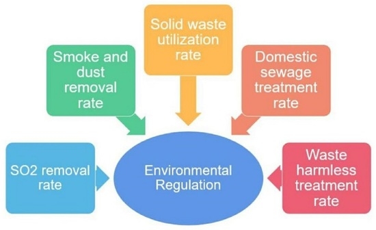
Explanatory variablesIndustrial SO2 removal rate (SO2)The intensity of environmental regulation is calculated by entropy weight method through the five single indexes of industrial SO2 removal rate (SO2), smoke and dust removal rate (dust), comprehensive utilization rate of industrial solid waste(solid), domestic sewage treatment rate (sewage) and harmless treatment rate of domestic garbage(garbage)
Smoke and dust removal rate (DUST)
Comprehensive utilization rate of industrial solid waste (SOLID)
Domestic sewage treatment rate (SEWAGE)
Harmless treatment rate of domestic garbage (GARBAGE)
Strength of environmental regulations (REGU)
Threshold variableRegional economy (GDP)GDP per capita
Control variableIndustrial structure (IS)Added value of tertiary industry/added value of secondary industry
Open to the outside world (FDI)Industrial output value of foreign-invested enterprises/Gross regional product
Government Action (GOV)The ratio of education and technology expenditure to the regional GDP
Infrastructure (ROD)Urban road area per capita
Innovation capacity (RD)Number of patents granted
Technology level (TECH)Power consumption per unit GDP
Table 2. Results of the threshold effect test: GDP as the threshold.
Environmental Regulation CategoryModelThresholdF-Statistic (F)p-Value (p)Bootstrap (BS)
REGUSingle threshold12,873125.74 ***0300
Double threshold12,87341.89 **0.0167300
55,447
Three thresholds19,82444.780.4367300
SO2Single threshold55,44763.23 ***0300
Double threshold12,87350.03 ***0.01300
55,447
Three thresholds35,333110.6833300
DUSTSingle threshold12,873119.26 ***0300
Double threshold12,87335.55 ***0.01300
55,447
Three thresholds19,82429.590.267300
SOLIDSingle threshold12,873104.01 ***0300
Double threshold12,87351.25 ***0. 0067300
55,447
Three thresholds19,82430.550.3367300
SEWAGESingle threshold12,87398.65 ***0300
Double threshold12,87352.41 ***0.0033300
55,447
Three thresholds17,59413.210.55300
GARBAGESingle threshold11,032113.26 ***0300
Double threshold11,03241.25 **0.0167300
55,447
Three thresholds19,82428.230.4567300
Note: *, **, and *** represent that the estimated coefficient is significant at the 10%, 5%, and 1% confidence levels, respectively.
Table 3. Parameter results of the model: GDP is the threshold.
VariableGDP is the Threshold
REGUSO2DUSTSOLIDSEWAGEGARBAGE
GDP-10.280 ***0.348 ***0.0160.105 *0.238 ***0.206 ***
(0.100)(0.096)(0.074)(0.059)(0.091)(0.074)
GDP-2−0.0250.002−0.166 ***−0.082 ***−0.075 *−0.06 *
(0.077)(0.046)(0.072)(0.020)(0.046)(0.035)
GDP-30.0630.126 ***−0.105−0.001 ***0.0150.008
(0.077)(0.046)(0.074)(0.000)(0.047)(0.038)
IS0.115 ***0.11 **0.114 ***0.12 ***0.115 ***0.117 ***
(0.042)(0.044)(0.041)(0.041)(0.041)(0.042)
FDI−0.061−0.068−0.054−0.066−0.051−0.058
(0.0645)(0.066)(0.065)(0.066)(0.065)(0.066)
ROD0.00110.00030.0020.0010.0020.001
(0.002)(0.002)(0.002)(0.002)(0.002)(0.002)
GOV0.624−0.1340.8310.6490.8270.59
(0.821)(0.873)(0.845)(0.811)(0.834)(0.783)
RD0.0095150.0050.01210.0080.0110.0108641
(0.022)(0.020)(0.022)(0.021)(0.022)(0.022)
TECH−0.258 **−0.232 *−0.28 ***−0.278 **−0.267 **−0.25 **
(0.120)(0.119)(0.123)(0.122)(0.121)(0.117)
Constant0.874 ***0.89 ***1. 007 ***0.923 ***0.896 ***0.906 ***
(0.063)(0.051)(0.08)(0.053)(0.055)(0.057)
Numbers163163163163163163
R-squared0.130.110.130.130.130.13
Note: *, **, and *** represent that the estimated coefficient is significant at the 10%, 5%, and 1% confidence levels, respectively. The standard errors of the coefficients are marked in parentheses.
Table 4. Threshold effect test results: NL (Nighttime light) is the threshold.
Environmental RegulationModelThresholdFPBS
REGUSingle threshold2.67044.95 *0.053300
Double threshold1.84540.550.137300
2.732
SO2Single threshold6.83461.99 ***0300
Double threshold2.67028.130.2333300
6.834
DUSTSingle threshold2.73248.21 **0.02300
Double threshold1.84540.20.13300
2.732
SOLIDSingle threshold1.84539.31 *0.093300
Double threshold1.84539.92 *0.083300
8.204
Three thresholds0.42833.940.383300
SEWAGESingle threshold8.48332.530.1833300
GARBAGESingle threshold2.67037.770.11300
Note: *, **, and *** represent that the estimated coefficient is significant at the 10%, 5%, and 1% confidence levels, respectively.
Table 5. Parameter results of the model: NL (Nighttime light) is the threshold.
VariableNL (Nighttime Light) Is the Threshold
REGUSO2DUSTSOLID
NL-10.090.09 *−0.0270.044
(0.077)(0.05)(0.070)(0.055)
NL-2−0.1220.14 **−0.182 **0.110 ***
(0.074)(0.059)(0.077)(0.038)
NL-3 0.001 **
(0.0003)
IS0.14 ***0.14 ***0.127 **0.121 ***
(0.037)(0.036)(0.036)(0.036)
FDI0.039−0.0190.0410.016
(0.054)(0.056)(0.055)(0.053)
ROD0.0020.0010.0020.002
(0.002)(0.002)(0.002)(0.002)
GOV0.484−1.19−0.538−0.766
(0.936)(0.808)(0.886)(0.84)
RD−0.001−0.017−0.002−0.008
(0.018)(0.015)(0.017)(0.015)
TECH−0.27 **−0.241 *−0.291 **−0.28 **
(0.136)(0.133)(0.137)(0.041)
Constant0.896 ***0.887 ***0.994 ***0.927 ***
(0.056)(0.046)(0.075)(0.055)
Numbers163163163163
Note: *, **, and *** represent that the estimated coefficient is significant at the 10%, 5%, and 1% confidence levels, respectively. The standard errors of the coefficients are marked in parentheses.
Table 6. Test results of threshold effect under lagging environmental regulation.
Environmental RegulationModelThresholdFpBS
REGU-1Single threshold12,14089.61 ***0 300
Double threshold11,15847.13 **0.0167 300
19,656
Three thresholds53,77131.50.39 300
SO2-1Single threshold12,14051.32 ***0.0033300
Double threshold12,14044.48 ***0.0067300
55,089
Three thresholds90,261120.6533300
DUST-1Single threshold17,42186.2 ***0300
Double threshold17,42132.66 **0.0233300
53,771
Three thresholds11,15826.540.2367300
SOLID-1Single threshold16,89280.96 ***0300
Double threshold16,89230.07 *0.0567300
61,177
Three thresholds11,15818.450.35300
SEWAGE-1Single threshold12,14066.11 ***0300
Double threshold12,14049.26 **0.0233300
55,089
Three thresholds19,65620.690.3867300
GARBAGE-1Single threshold12,14081.4 ***0300
Double threshold12,14033.37 *0.06300
53,771
Three thresholds19,65628.280.23300
Note: *, **, and *** represent that the estimated coefficient is significant at the 10%, 5%, and 1% confidence levels, respectively.
Table 7. Parameter results of the model under lagging environmental regulations.
VariableEnvironmental Regulation Lags One Step Behind
REGU-1SO2-1DUST-1SOLID-1SWAEGE-1GARBAGE-1
GDP-10.5137 ***0.364 ***0.050.140 ***0.271 ***0.153 **
(0.123)(0.124)(0.0795)(0.045)(0.096)(0.070)
GDP-20.228 ***−0.061−0.174 **−0.005−0.043−0.074 **
(0.072)(0.070)(0.078)(0.005)(0.045)(0.034)
GDP-30.0680.102 **−0.1140.067 ***0.047−0.013
(0.067)(0.044)(0.080)(0.020)(0.043)(0.036)
IS0.113 **0.115 **0.113 ***0.118 ***0114 **0.12 ***
(0.044)(0.013)(0.043)(0.043)(0.044)(0.045)
FDI−0.033−0.061−0.047−0.060−0.055−0.06
(0.069)(0.07)(0.0696)(0.070)(0.071)(0.07)
ROD0.0030.0010.0020.0020.0010.002
(0.002)(0.002)(0.002)(0.002)(0.002)(0.002)
GOV1.3960.3410.9220.7110.6760.790
(0.845)(0.831)(0.293)(0.847)(0.772)(0.779)
RD0.0220.0090.01550.0130.0120.0131
(0.022)(0.02)(0.021)(0.021)(0.021)(0.021)
TECH−0.428 ***−0.301 **−0.381 **−0.365 **−0.286 **−0.310 **
(0.155)(0.13)(0.150)(0.14)(0.125)(0.128)
Constant0.799 ***0.883 ***1.01 ***0.86 ***−0.286 **0.911 ***
(0.062)(0.054)(0.085)(0.052)(0.125)(0.057)
Numbers163163163163163163
Note: *, **, and *** represent that the estimated coefficient is significant at the 10%, 5%, and 1% confidence levels, respectively. The standard errors of the coefficients are marked in parentheses.
Publisher’s Note: MDPI stays neutral with regard to jurisdictional claims in published maps and institutional affiliations.

