Performance Analysis of Air Cooled Heat Pump Coupled with Horizontal Air Ground Heat Exchanger in the Mediterranean Climate

Abstract

A concept of Air-Cooled Heat Pump (ACHP) coupled with a Horizontal Air-Ground Heat Exchanger (HAGHE), also called Horizontal Earth-To-Air Heat Exchanger (EAHX), has been proposed. The Air-Cooled Heat Pump is a system which transfers heat from outside source (air) to inside sink (water) and vice versa in summertime. The innovation is to provide a geothermal treatment of pre-heating/cooling of air before meeting the evaporator in winter or the condenser in summer of the heat pump. Besides, it is known that the variations of the ground temperature, respect to the external air one, are mitigated already in the first layers of the ground throughout the year, due to the high thermal inertia of the ground, letting the heat pump work with more mitigated conditions, improving the performances. The behaviour of HAGHE has been investigated by varying the length and the installation depth of the probes, the air flow rate and the ground thermal properties. All the combinations have been implemented using TRNSYS 17 software (Transient System Simulation Program) to obtain the outlet temperatures from HAGHE, resulting from the 54 configurations. The results are compared in terms of Coefficient of Performance (COP) in wintertime and Energy Efficiency Ratio (EER) in summertime between configurations with and without the coupling with HAGHE. In addition, two seasonal performance SCOP and SEER coefficients have been calculated considering, not only the inlet air temperatures into the Air-Cooled Heat Pump, but also their frequency of occurrence, the off-set external temperature (16 °C), the nominal external temperature and heating and cooling loads.

1. Introduction

The energy efficiency of building sector is one of the most key issues about the energy policies of the European Union, since the construction sector constitutes 40% of the global energy consumptions in the developed territories. The European Commission has fixed the goals to encourage an intelligent, sustainable and inclusive growth with the climate and energy package called “20-20-20”. In the climate and energy sectors the aims of the EU 20-20-20 become an important status considering the necessity to cut the gas emissions of 20%, as well as to cover the 20% of the final energy consumptions with renewable energy sources, and to improve the energy efficiency of 20%. By 31 December 2020, all new buildings must be ZEBs (Zero Energy Buildings) or nZEBs (Nearly Zero Energy Buildings) and those occupied and owned by public authorities must comply with the same criteria by 31 December 2018, for the assertions of the European Directive 31/2010 [1]. UE puts in evidence the significance of reaching smart growth with simultaneous reduction of energy consumptions and investment and maintenance costs, through the strengthening of energy efficiency measures and the adoption of many policies in this regard.

Since the 11% of world energy produced is used in the buildings for cooling and heating [2], for this reason it has been considered crucial the necessity to investigate innovative solutions for HVAC (Heating, Ventilating and Air Conditioning).

A technology that could potentially contribute significantly to reducing energy consumption in the civil sector is represented by geothermal heat pump systems. These plants, in fact, currently constitute a valid alternative, both in terms of energy and economy, to traditional air conditioning systems.

Besides, in 2018, the negotiation process for the European Union’s post-2020 climate and energy framework is coming to an end [3]. The debate had recognised geothermal as a relevant energy source for the future of Europe. Within the last five years, after nearly a decade of only small development in Europe, it has been noted an increasing interest in geothermal power and heat. Several projects have been carried out in Europe, and geothermal energy is on its way to become a key player in the European energy market.

A new generation of geothermal technologies is also needed for answering the challenges that the European energy system will face in the next few decades.

If the energy transition is to be successful, it will be necessary to define optima scenario in terms of costs and affordability, for customers and citizens. As a local and stable source of renewable energy, geothermal will be a key enabler for the decarbonisation of the economy and with a crucial role to play in the future energy system.

This study aims to demonstrate how it is possible to increase the performances of an air-cooled heat pump with the use of Horizontal Air-Ground Heat Exchangers (HAGHE). The proposed innovation is to use HAGHE, not only for the typical application of air ventilation treatment, but for the treatment of the external air before working on the heat pump. It is provided a geothermal treatment for the pre-heating/cooling of air before meeting the evaporator in winter or the condenser in summer, working with colder and warmer air than external air, respectively.

Literature Overview

In literature, there are many articles that concern the behaviour of Water-Cooled Heat Pumps. The increase of the Coefficients of Performance (COP) in Ground Source Heat Pump (GSHP) system, both in summer and in winter, involves the reduction of consumption and emission compared with the traditional heat pump [4].

Desideri et al. [5] show that the costs of heating operation with a methane boiler are higher than those necessary to heat the building with the GSHP. In literature, there are researches mainly on the use of horizontal water ground heat exchangers [6].

Galgaro et al. [7] proved that the Ground Heat Exchanger (GHE), coupled with heat pumps, assures energy efficiency far greater than air-source systems. Baccoli et al. [8] considered the energy analysis of a heat pump system coupled with vertical exchangers, to verify which the exploitation of atmospheric air makes it competitive in comparison with other technologies.

To define the system performance, different configurations of horizontal water ground heat exchangers are compared by Congedo et al. [9]. Wu et al. [10] considered the thermal performance of slinky heat exchangers of horizontal-coupled GSHP in a UK climate.

There are few researches concerning the analysis of Horizontal Air-Ground Heat Exchangers (HAGHEs).

It is noted that using the thermal energy stored in the ground, it is possible to pre-heat or pre-cool the ventilation air, in winter and summer, respectively. Previous studies demonstrate that a good reduction of CO₂ gas emissions results from the replacement of traditional air heat pumps with to Ground Source Heat Pump (GSHPs) [11]. Even Saner et al. [12] showed a reduction of up to 90% of CO₂ emissions compared to natural gas boilers.

Congedo et al. [13] show that HAGHE has good performance in terms of high efficiency with a low environmental impact, operating on the ventilation air, using a pipe only 5 m long in the simulations. The geothermal heat exchanger horizontal air-to-ground (HAGHE) is a simple superficial system. It consists of pipes which are buried in the ground at the depth of about 2.5 m, with outside air like vector fluid. For more applications, it is necessary to know the influence of each parameter on the thermal performance of HAGHE, as well as the pipes configuration and the ground properties [13]. The horizontal geometry of pipes outperforms the vertical configuration, the first one has not the problems related to deep wells, like cost and risk to meet the aquifer.

2. Proposed Solution: Air-Cooled Heat Pump Coupled with Horizontal Air Ground Heat Exchanger

A coupling system between Air Cooled Heat Pump (ACHP) and HAGHE, applied in a warm climate, has been proposed. The behaviour of the heat pump is represented by the coefficients COP, EER, SCOP and SEER. The comparison is carried out between the standard behaviour of the heat pump and the performances of the ACHP-HAGHE. The HAGHE System has been modelled with the use of TRNSYS 17 software (TRaNsient SYStem, developed by the University of Wisconsin, Madison, WI, USA) to evaluate the influence of geometrical and thermal variables of HAGHE system.

The innovation provides a geothermal treatment of pre-heating/cooling of external air before meeting the evaporator in winter or the condenser in summer of the Air-Cooled Heat Pump.

In other words, the paper presents the results obtained from the comparison of the indexes of performance, COP and EER of the air-cooled heat pump considering, like cooling vector, external air with and without the treatment through a HAGHE, varying the air flow rate for single pipe, the length and burial depth of the pipe and the ground thermal properties, along one year by unsteady simulations using annual weather data.

The analysis has been carried out in the city of Brindisi, located in the South of Italy, that has 1083 heating degrees days and cooling degree days equal to 299 (Italian climatic zone C). It is characterized by a Mediterranean climate with by non-extreme winters (average temperature 13 °C over the last ten years), high aridity in summer (average temperature 30.3 °C) and rainfall concentrated in autumn and winter [14,15]. The annual solar irradiation on horizontal surfaces in Brindisi is equal to 1582 kWh/m²(minimum value), 1610 kWh/m² (mean value) and 1620 kWh/m² (maximum value).

The operative air temperature to guarantee a thermal comfort for the end users is 20 °C during the heating period (15 November to 31 March) and 26 °C during the cooling period [16].

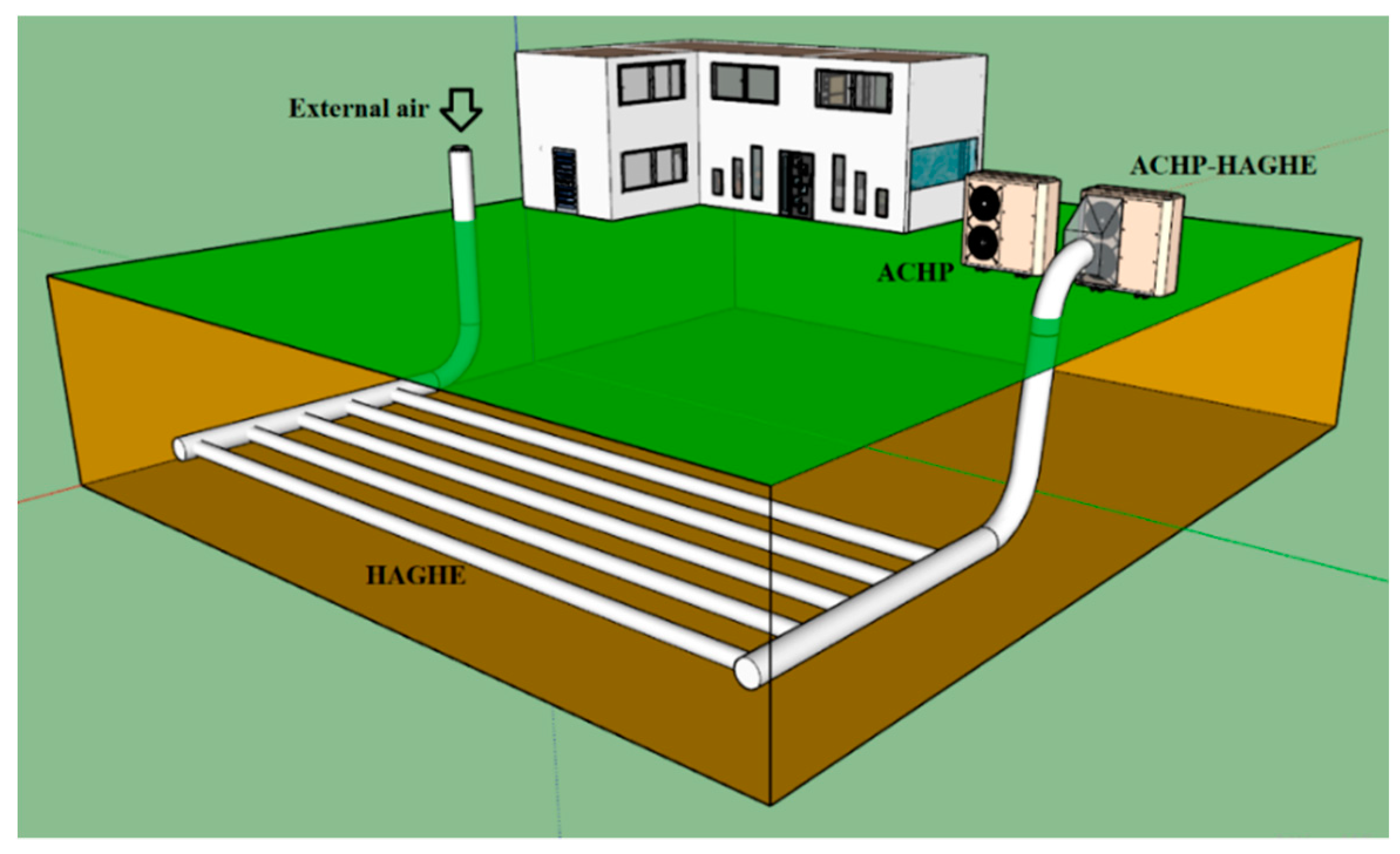
This study employs the ground temperature behaviour that, below a certain depth, remains relatively constant throughout the year. Therefore, at enough depth, the ground temperature is higher than the external one in winter and lower in summer. The difference of temperature between the external air and the ground can be used to preheat the air flow rate in winter and pre-cool it in summer by HAGHE. The ACHP-HAGHE system proposed is shown in Figure 1, compared with an ACHP in standard configuration.

HAGHE, basically, consists of horizontal probes which are buried in the ground, coupled with an air system which forces the outside air through the probes. Parameters such as the probes layout and the ground properties can affect the heat transfer that characterize a geothermal heat exchanger, that taking place by convection between the air and the surfaces of the probe, and by conduction, towards the nearest ground.

2.1. Geothermal Probe

Table 1. Configuration parameters for HAGHE simulations.

Probe Properties	Probe Length		10	m
			30	m
			50	m
	Nominal Diameter		0.5	m
	Inner Diameter		0.466	m
	Outer Diameter		0.517	m
	Thermal Conductivity of Probe Material		0.40	W/mK
	Number of Probes		16 (G = 825 m3/h)	-
			13 (G = 1015 m3/h)	-
			11 (G = 1200 m3/h)	-
	Burial Depth		2	m
			3	m
	Distance between the Probes Axes		1.5	m
Air Properties	Air Flow Rate (G)		825	m3/h
			1015	m3/h
			1200	m3/h
	Density of Air		1.205	kg/m3
	Thermal Conductivity of Air		0.026	W/mK
	Specific Heat of Air		1.005	kJ/kgK
	Viscosity of Air		1.81 × 10−5	kg/ms
Ground Properties	Ground volumetric humidity = 0%	Ground Thermal Conductivity	0.26	W/mK
		Density of Ground	1600	kg/m3
		Specific Heat of Ground	0.8965	kJ/kgK
	Ground volumetric humidity = 20%	Ground Thermal Conductivity	1.18	W/mK
		Density of Ground	1800	kg/m3
		Specific Heat of Ground	1.2586	kJ/kgK
	Ground volumetric humidity = 40%	Ground Thermal Conductivity	1.591	W/mK
		Density of Ground	2000	kg/m3
		Specific Heat of Ground	1.5655	kJ/kgK
	Average Surface Temperature		16.7	°C
	Amplitude of Surface Temperature		18.7	°C
	Time Shift		45	day
Finite elements calculation set up	Number of Fluid Nodes		100 (L = 10 m)	-
			300 (L = 30 m)	-
			500 (L = 50 m)	-
	Number of Radial Ground Nodes		−1	-
	Number of Axial Ground Nodes		20	-
	Number of Circumferential Ground Nodes		8	-
	Smallest Node Size		0.2	m
	Node Size Multiplier		1.2	-
	Farfield Distance		1	m
	Initial Temperature of Air		10.1	°C

shows the properties of probes, air and ground and the finite elements calculation set up in TRNSYS. The parameters of Kusuda-Achenbach ground temperature model are shown. The material of the probe is polyethylene, characterized by a thermal conductivity equal to 0.4 W/mK. The length of the probes has been simulated considering three different length values equal to 10 m, 30 m and 50 m, changing the number of fluid nodes on the TRNSYS set up. Another variable which has been tested is the number of probes equal to 16, 13, 11 and the resulting air flow rate equal to 825 m³/h, 1015 m³/h, 1200 m³/h, respectively.

The investigation included two different values of ground burial depth (2 m and 3 m) and three ground volumetric water contents equal to 0%, 20% and 40% to which correspond, respectively, three values of ground thermal conductivities, ground specific heats and densities. COP and EER of ACHP are calculated hourly, for one year, in the following periods: - in winter, from 15 November to 31 March; - in summer, from 1 June to 31 August. The working time of the system has been set considering a typical office opening time, from 8.00 am to 6.00 pm.

2.2. Air Cooled Heat Pump

The study focuses on a commercial single-circuit Air-Cooled Heat Pump suitable for residential and commercial uses. It is characterized by a maximum thermal power equal to 30 kW and it is charged with R410A gas. The system can be connected to fan coil terminals or to a low temperature radiant system. The inverter permits to continuously modulate the heating and cooling power from 25% to 100%, to respond promptly to user requests.

The heat pump processes a total of 13,200 m³/h of air flow rate. The number of probes of the system varies in accordance with the air flow rate of each probe (825–1015–1200 m³/h each one), like shown in Table 1.

In function of the presence of low or medium temperature heating systems (such as radiant floors or fan-coils), the heat pump can heat the thermal water until 35 °C or 55 °C. As regard the summer season, the heat pump behaves like a chiller, cooling the water until 6 °C and 10 °C.

The COP (Coefficient of Performance) is the ratio between the thermal power delivered to the system and the electrical power consumed by the heat pump. This indicator is useful to compare the efficiency of various heat pumps. COP can be expressed by the formula:

COP = h_h/P_e

(1)

where h_h is the produced heat and P_e is the electrical power of the considered system.

Similarly, the cooling efficiency of the heat pump, expressed by the Energy Efficiency Ratio (EER), is calculated as shown below:

EER = h_c/P_e

(2)

where h_c is the cooling heat and P_e is the electrical power.

2.2.1. SCOP

The Seasonal Coefficient of Performance (SCOP) permits to evaluate, with greater accuracy, the working conditions of heat pump. Several parameters affect the seasonal performance, such as the quality of the heat pump, the climatic conditions, the installation site and the heating system to which the heat pump is connected.

Regarding the Heat Pumps (aeraulic, geothermal and hydraulic) is essential to consider the UNI 11300-4 [17] at the paragraph «Reduced load factor performance» and the reference to UNI EN 14825 [18]. The legislation provides for the seasonal performance index (SCOP) to be calculated with the “bin method” (frequency method of occurrence of the temperature), distributed for the entire heating season. The climatic condition of Brindisi can be considered as intermediate average conditions (W), in accordance with the classification that provides the following classification:

−

A (Average): Strasbourg (France); external design temperature = −10 °C

−

C (Colder): Helsinki (Finland); external design temperature = −22 °C

−

W (Warmer): Athens (Greece); external design temperature = +2 °C

These climate conditions are considered sufficiently representative of the climate of all Europe. Once defined the climatic representative condition, it is possible to identify the different parameters for the SCOP calculation. The W (Warmer) climate presents the external design temperature equal to = +2 °C.

The «PLR» climate load factor (Part Load Ratio) describes the relationship between the partial load (or total load) divided by the full load.

$$\mathrm{PLR}=\frac{{\mathrm{T}}_{\mathrm{est}}-{\mathrm{T}}_{\mathrm{off}}}{{\mathrm{T}}_{\mathrm{est},\mathrm{des}}-{\mathrm{T}}_{\mathrm{off}}}=\frac{{\mathrm{T}}_{\mathrm{est}}-16}{0-16}$$

(3)

The internal design temperature is considered equal to 20 °C, while the Temperature of Balance (T_off) is 16 °C, meaning that the operation stops heating system for outdoor temperature greater than 17 °C.

In accordance with the UNI EN 12831-1:2018 [19], the project parameter (T_{est, des}) for the city of Brindisi is 0 °C.

The PLR value ranges from 0 (when the user heating demand is null) to 1 (when the heating demand is maximum).

This study provides the calculation of the SCOP_on (Seasonal performance coefficient active operation) which evaluates the active operating period including consumption due to possible additional electric heaters. It differs from the SCOP_net (Net seasonal performance coefficient), i.e., the seasonal performance coefficient which considers the active operating period excluding consumption due to possible additional electric heaters.

The SCOP_on is calculated as follows:

$${\mathrm{SCOP}}_{\mathrm{on}}=\frac{{{\displaystyle \sum }}_{\mathrm{j}=1}^{\mathrm{n}}\mathrm{hj}\ast \mathrm{Ph}\left(\mathrm{Tj}\right)}{{{\displaystyle \sum }}_{\mathrm{j}=1}^{\mathrm{n}}\mathrm{hj}\left(\frac{\mathrm{Ph}\left(\mathrm{Tj}\right)-\mathrm{elbu}\left(\mathrm{Tj}\right)}{{\mathrm{COP}}_{\mathrm{PL}}\left(\mathrm{Tj}\right)}+\mathrm{elbu}\left(\mathrm{Tj}\right)\right)}$$

(4)

With Q_des equal to 30 kW.

2.2.2. SEER

The Seasonal Energy Efficiency Ratio index (SEER) considers the variation in electrical absorption depending on the boundary conditions and the degree of partialization of the machine.

To take into account the variation in electrical absorption depending on the climatic conditions (and/or of the boundary conditions) and the degree of partialization of the machine, the SEER index is calculated as weighted mean of the individual EERs at different operating conditions, using operating weights and times defined on a conventional basis (bin-method), depending on the type of machine [18].

The primary energy requirement for summer air conditioning is determined as the sum of the contributions (corrected for the conversion factor to electricity from primary energy) of the electricity needs of the auxiliaries for cooling and for air treatments.

The SEER_on is determined as follows:

$${\mathrm{SEER}}_{\mathrm{on}}=\frac{{{\displaystyle \sum }}_{\mathrm{j}=1}^{\mathrm{n}}\mathrm{hj}\ast \mathrm{Pc}\left(\mathrm{Tj}\right)}{{{\displaystyle \sum }}_{\mathrm{j}=1}^{\mathrm{n}}\mathrm{hj}\ast \frac{\mathrm{Pc}\left(\mathrm{Tj}\right)}{\mathrm{EERbin}\left(\mathrm{Tj}\right)}}$$

(5)

The external design temperature (T_{est, des}) for Brindisi is 37.1 °C as reported in UNI EN ISO 13789:2018 [20]. The internal design temperature is 20 °C. The Temperature of Balance (T_off) is 16 °C, meaning that the operation stops cooling system for outdoor temperature lower than 15 °C.

As reported in (6), the PI (Part Load Ratio) defines the relationship between the partial load (or total load) divided by the full load.

$$\mathrm{PI}=\frac{{\mathrm{T}}_{\mathrm{est}}-16}{37.1-16}$$

(6)

3. Calculation

The software TRNSYS 17 may be used to simulate the HAGHE system in order to obtain the outlet temperature of the treated air [21]. A total of 54 combinations have been considered, varying the length and the installation depth of the probe, the air flow rate and the ground thermal properties. The analysis of the HAGHE have been done for 8760 h (365 days), despite the ACHP system is on and off alternately throughout the year. The heating and cooling operating periods are reported in Section 2.1.

Generally, the off-period of the HAGHE guarantees the ground regeneration. The choice to consider the HAGHE working throughout the year, despite the shutdown of the ACHP, is conservative and precautionary. In addition, this choice permits to monitor the ground thermal inertia and to investigate the behaviour of the HAGHE also for other application during the periods of the year in which the ACHP is off.

For each water temperature, the COP and EER have been calculated considering the outlet temperature of treated air from HAGHE compared with the traditional system, which uses the external air.

Besides, the seasonal performance SCOP and SEER coefficients have been calculated in function of the inlet air temperatures into the ACHP, their frequency of occurrence, the off-set external temperature (16 °C), the nominal external temperature and heating and cooling loads.

3.1. HAGHE Modelling by “TRNSYS 17”

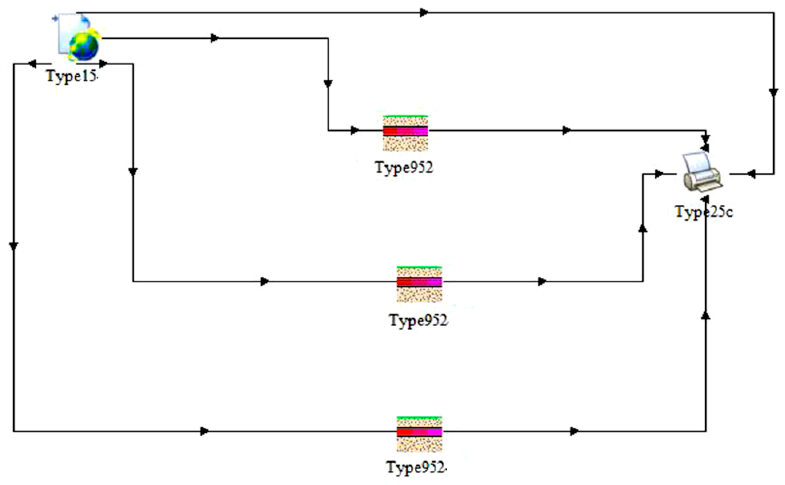
In this section, it is presented the model that represents the behaviour of the Air-Ground Heat Exchanger designed in TRNSYS 17. TRNSYS is a transient system simulation program with a modular structure. It allows the user to describe the system by connecting the components that constitute the simulation. The TRNSYS library includes many of the components commonly found in thermal and electrical energy systems, as well as component routines to handle input of weather data or other time-dependent forcing functions and output of simulation results. Figure 2 shows the set-up scheme of the HAGHE model reproduced in TRNSYS environment.

The weather data of the city of Brindisi are generated by Meteonorm, which are included in the Type 15. Meteonorm is a database of meteorological information, which provides data and calculation procedures for several locations, based on statistical data. The Type 952 (Single Pipe System in GHP, Geothermal Heat Pump Library) models the probe buried under the ground surface. The probe is surrounded by a 3-Dimensional finite difference conduction network to calculate the heat build-up in the ground. This subroutine models the yearly values of the vertical temperature of the ground surface, the amplitude of the ground surface temperature (that indicates the difference between the maximum temperature and the mean temperature), the time difference between the beginning of the calendar year and the occurrence of the minimum surface temperature (Time shift) and the thermal diffusivity of the ground. Table 1 shows the setup parameters of Type 952. The “Number of Radial Soil Nodes” has been set equal to −1 in order to calculate the radial noding pattern based on an expanding multiplier.

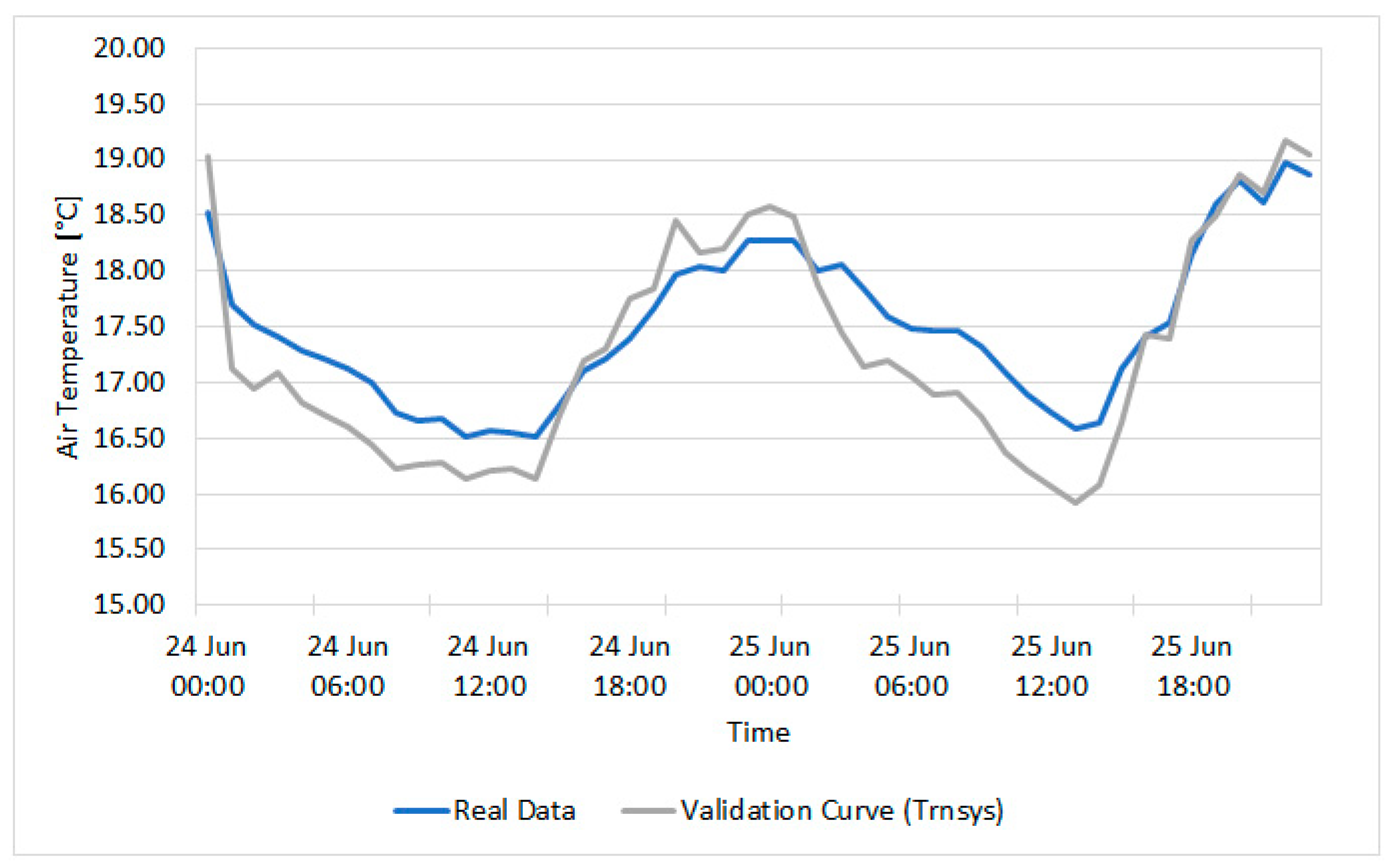
The model developed with TRNSYS has been validated with a real case study of building placed in Rubiana (Turin) [22]. Type 15 has been replaced by the real climatic data of the city. Type 952 contains the real characteristics of the probes in terms of diameter equal to 0.25 m and length of 48 m, the burial depth is equal to 3.15 m and the ground humidity of 10%. The air flow rate analysed is equal to 450 m³/h.

Figure 3 shows the comparison between the outgoing temperatures from the probe for 48 h (24 June and 25 June). The blue curve represents the real temperatures measured with the sensor installed inside the probe, the grey one is the trend of data resulting by TRNSYS model.

As shown in Figure 3, the trend of experimental and numerical data are very similar. The maximum deviation is 0.71 °C (24 June at 12 a.m.) while the average deviation for the entire period of 48 h is 0.23 °C.

3.2. COP and EER at Maximum Frequency

The COP and EER values depend on the outside air temperature and the water temperature to be produced (Data declared according to UNI EN 14511-2:2011 [23]).

Table 2. Equations of the COP as function of the Air Temperature T (T_Aext or T_Aout) and the Water treated Temperature (T_w) at the maximum frequency.

Tw (°C)	Function of Trend Line COP (T)	R²
35A [Air Temperature −15;3]	COP(T) = 5 × 10−7T6 + 2 × 10−5T5 + 0.0003T4 + 0.0017T3 + 0.009T2 + 0.078T + 2.5019	0.9951
35B [Air Temperature 3;20]	COP(T) = −2 × 10−7T6 + 2 × 10−5 T5 − 0.0004T4 + 0.0066T3 − 0.0606T2 + 0.4206T + 2.0482	0.9997
45A [Air Temperature −15;3]	COP(T) = 3 × 10−7T6 + 1 × 10−5T5 + 0.0002T4 + 0.0013T3 + 0.008T2 + 0.0571T + 2.0009	0.9959
45B [Air Temperature 3;20]	COP(T) = −2 × 10−7T6 + 1 × 10−5T5 − 0.0003T4 + 0.0051T3 − 0.0487T2 + 0.3524T + 1.5977	0.9993
55A [Air Temperature −15;3]	COP(T) = −4 × 10−7T6 – 9 × 10−6T5 − 6 × 10−5T4 + 0.0002T3 + 0.0062T2 + 0.0429T + 1.6694	0.9957
55B [Air Temperature 3;20]	COP(T) = −2 × 10−7T6 + 1 × 10−5T5 − 0.0004T4 + 0.0057T3 − 0.0527T2 + 0.358T + 1.213	1

and

Table 3. Equations of the EER as functions of the Air Temperature T (T_Aext or T_Aout) and the Water treated Temperature (T_w) at the maximum frequency.

Tw (°C)	Function of Trend Line EER (T)	R²
2	EER(T) = −1 × 10−5T3 + 0.0023T2 – 0.1808T + 6.2089	1
6	EER(T) = −4 × 10−5T3 + 0.005T2 – 0.2806T + 7.7483	1
10	EER(T) = −5 × 10−5T3 + 0.0063T2 – 0.3423T + 8.9556	1

show the equations of COP and EER at the maximum frequency, with the corresponding regression coefficient R². The R² coefficients ranges between 0 and 1, this means that how much more the R² values tend to 1, the more the model best analyses the data.

As regards the COP, the Sixth-degree equations are obtained from the trend lines. It has been noted that a single trend line does not perfectly represent the behavior of the COP, for this reason it was decided to build two trend lines (A and B) for each curve to obtain more consistent results. Therefore, two sixth grade equations were obtained for each curve. The behavior of the EER is represented by third-order polynomial trend lines.

4. Analysis of Results

All results are used to calculate the performances of the ACHP in terms of COP, EER, SCOP and SEER. In all graphs reported below, the coupled system is compared with the traditional one, analysing every time the performance of the heat pump with the treated air from the HAGHE and the heat pump with the external air.

4.1. Treated Air Temperature

In

Table 4. External air temperatures (°C) and treated air temperatures outgoing from HAGHE.

				TAext (°C)	TAout (°C)
Ground Volumetric Humidity	Date	H (m)	G		L = 10 m	L = 30 m	L = 50 m
			(m3/h)
40%	14 February 7 a.m.	2	833.33	1.1	2.5	4.9	6.6
			1041.67	1.1	2.3	4.5	6.2
			1250	1.1	2.2	4.2	5.8
		3	833.33	1.1	2.9	5.9	8.2
			1041.67	1.1	2.7	5.4	7.6
			1250	1.1	2.5	5.1	7.1
	21 July 4 p.m.	2	833.33	35.5	33.2	29.7	27.1
			1041.67	35.5	33.4	30.3	27.8
			1250	35.5	33.6	30.7	28.4
		3	833.33	35.5	32.9	28.9	25.9
			1041.67	35.5	33.2	29.6	26.7
			1250	35.5	33.4	30.1	27.4
20%	14 February 7 a.m.	2	833.33	1.1	2.4	4.6	6.3
			1041.67	1.1	2.2	4.3	5.8
			1250	1.1	2.1	4.0	5.5
		3	833.33	1.1	2.7	5.5	7.7
			1041.67	1.1	2.5	5.1	7.1
			1250	1.1	2.4	4.7	6.6
	21 July 4 p.m.	2	833.33	35.5	33.4	30.2	27.7
			1041.67	35.5	33.6	30.7	28.4
			1250	35.5	33.8	31.2	29.0
		3	833.33	35.5	33.1	29.4	26.6
			1041.67	35.5	33.4	30.1	27.4
			1250	35.5	33.6	30.6	28.1
0%	14 February 7 a.m.	2	833.33	1.1	1.9	3.6	4.9
			1041.67	1.1	1.8	3.2	4.4
			1250	1.1	1.7	2.9	4.0
		3	833.33	1.1	2.0	3.7	5.2
			1041.67	1.1	1.8	3.3	4.7
			1250	1.1	1.7	3.1	4.2
	21 July 4 p.m.	2	833.33	35.5	34.2	32.2	30.4
			1041.67	35.5	34.4	32.7	31.1
			1250	35.5	34.6	33.0	31.6
		3	833.33	35.5	34.2	32.1	30.2
			1041.67	35.5	34.4	32.6	31.0
			1250	35.5	34.5	33.0	31.5

are reported the external air temperatures (T_Aext) and outlet temperatures of treated air from HAGHE (T_Aout). The treated air temperatures have been calculated considering the ground volumetric water content (0%, 20% and 40%) and the probe length L ranging from 10 m to 50 m. The results have been represented for the 14th February and 21 July, the coldest and the hottest day of the year, respectively.

From Table 4 it may be seen that, in winter, the treated air temperature increases and, in summer, decreases when the probe length increases, the air flow rate decreases and the ground burial depth increases. The temperature of the ground increases during the winter and it decreases in summer as the depth increases.

An additional comparison can be done by varying the ground volumetric humidity (0–40%), corresponding to different values of ground thermal conductivity, density and heat capacity, like shown in Table 1. Table 4 underlines that as ground volumetric humidity increases, the outlet air temperature from the probe increases in winter and decreases in summer, corresponding to a general improvement of the ACHP-HAGHE performances.

Finally, the influence of the length of the probe has been investigated. As already mentioned, the outlet air temperature increases or decreases, in winter and summer respectively, as the probe length increases. The greater heat exchange occurs in the first meters (20–30 m) of the probe, thus a probe of 50 m is not economically advantageous. In fact, it is more convenient to split 50 m in two probes of 25 m working in parallel, respect to the single probe of 50 m, because the first section works with the highest value of temperature difference between air and ground.

For this reason, this work has been developed using probes with a length of 30 m and only the last comparison has been done with the 50 m probes.

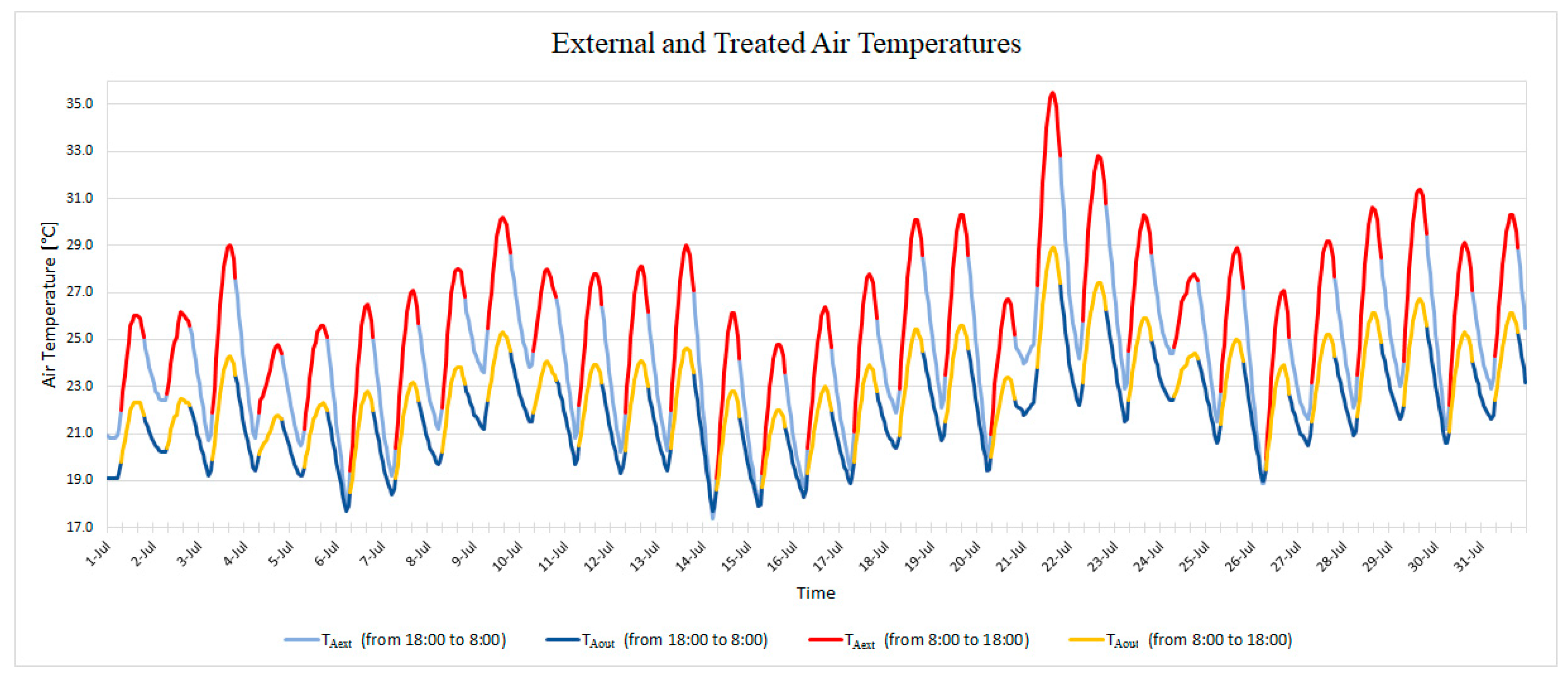
The geothermal probes can be easily converted in a free-cooling ventilation system using a bypass in the middle seasons when the heat pump does not work, but not only. In fact, every day, it is possible to switch the geothermal probes from the heat pumps to the ventilation system when the heat pumps don’t work (18:00–8:00).

Figure 4 points out the comparison between the external air temperature (T_Aext) and the treated air temperature (T_Aout) from the geothermal probes. The curves of T_Aext and T_Aout have been split in two time intervals from 8:00 to 18:00 (red line for external air and yellow line for treated air) and from 18:00 to 8:00 (light blue line for external air and blue line for treated air). The analysis is carried out for the all hours of July. As regards the geothermal system represented in Figure 4, the air flow rate equal to 825 m³/h, the burial depth of 3 m, the ground humidity of 40% and length of the probe of 30 m have been used.

As shown in Figure 4, the treated air temperature is considerably lower than the external one, especially during the night hours, and it allows to use free cooling coupled with probes to drop the internal temperature of the building. The day after, the ACHP-HAGHE system starts to work to cover the thermal load of a cooler building.

4.2. Comparison of COPs

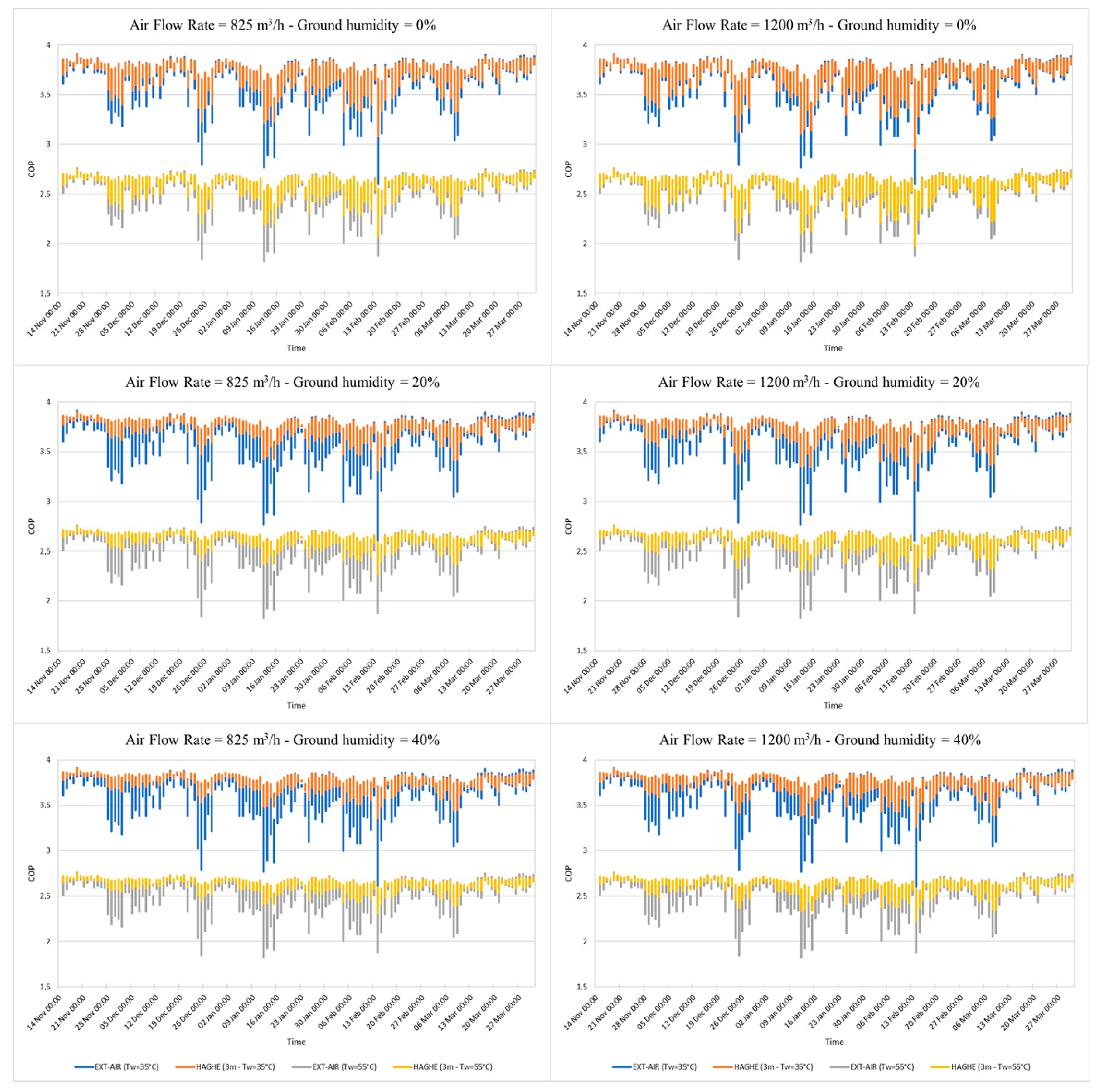
Figure 5 summarizes the comparison of the COP curves for the entire period of the winter season, from 15 November to 31 March, by varying the parameters described above (ground thermal properties, burial depth, air flow rate and ground volumetric humidity).

Each graph consists of two curves, the blue curve shows the COP of ACHP, in traditional configuration, that exchanges with the external air (COP_EXT-AIR), while the orange curve represents the COP of ACHP, coupled with HAGHE, working with the treated air by the geothermal probe (COP_HAGHE). Figure 5 shows the COP trends with an air flow rate of 825 m³/h and 1200 m³/h, respectively, by varying the ground volumetric humidity (0–20–40%) at burial depth of 3 m.

The curves show the COP trends for different water temperatures, treated by ACHP, for radiant floors equal to 35 °C and 55 °C for fan coils.

The COP_HAGHE are, on average, higher than COP_EXT-AIR and show a behavior with smaller oscillations. Of course, with lower water temperatures (35 °C), COPs are significant higher respect to COPs for a water temperature higher (55 °C). Ground volumetric humidity shows a slow influence, varying between 20–40%.

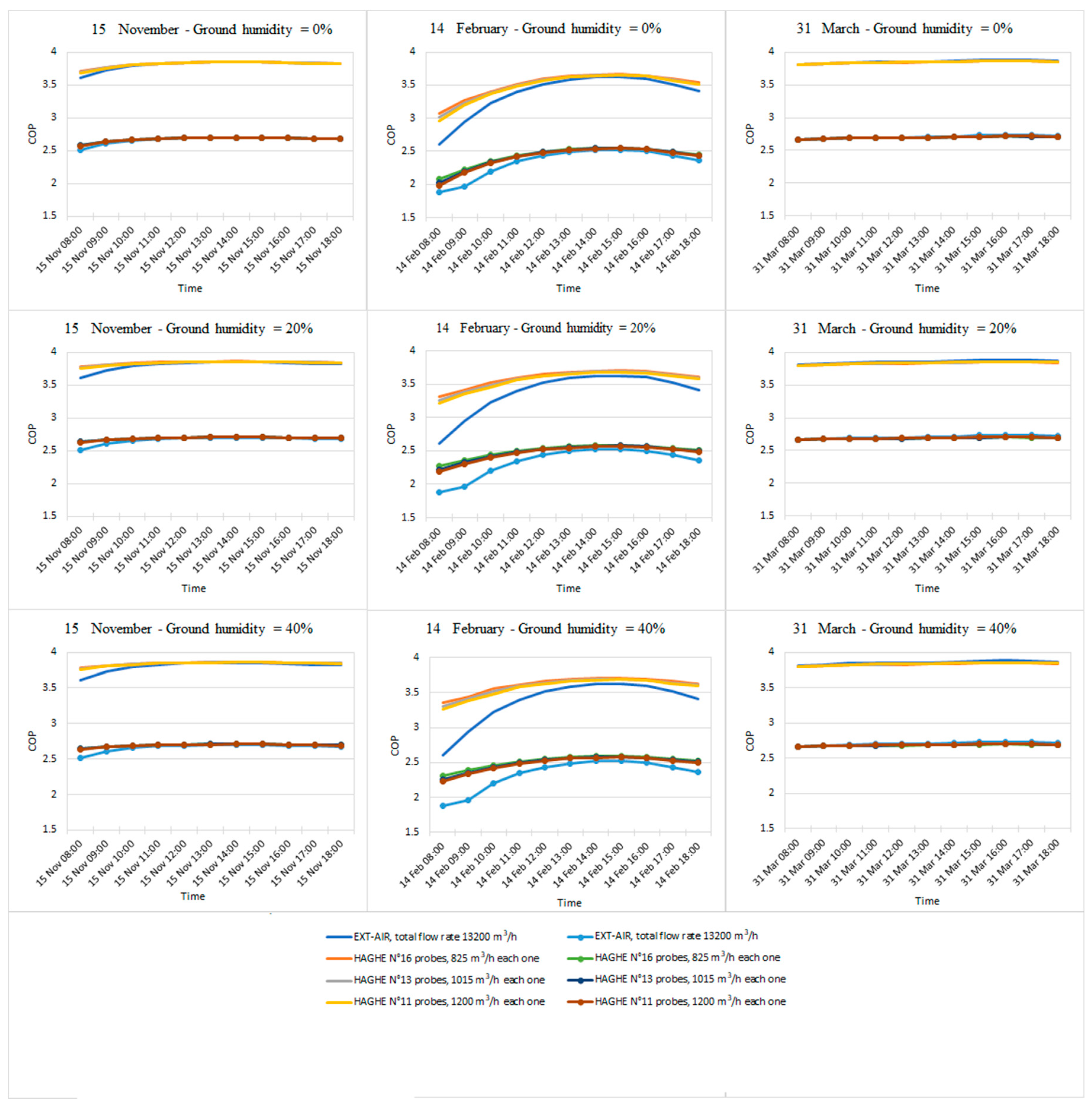
In Figure 6 is reported the comparisons for three selected days:

−

15 November (first day with air conditioning system turned on);

−

14 February (the coldest day);

−

31 March (last day with air conditioning system turned on).

for the temperature of the treated water at 35 °C and 55 °C for three air flow rates selected and three ground volumetric humidities.

On the left, Figure 6 shows that, during the 15 November, COP_HAGHE has an improvement only in the early hours of the day and it becomes negligible later.

About the day 14 February (in the middle of Figure 6), good results have been obtained in all cases, but in the central hours of the day it is noted that the difference between COP_HAGHE and COP_EXT-AIR for each air flow rate is small.

Regarding the date of 31 March (on the right of Figure 6), the COP_HAGHE has values almost coincident to the COP_{EXT AIR} in the entire range of temperatures analysed. The use of geothermal probes does not highlight any particular improvements. The combination that connotes the highest value of COP_HAGHE is defined by a burial depth of 3 m, a 30 m probe length, an air flow rate equal to 825 m³/h, a ground volumetric humidity of 40%, in particular with radiant floors, considering a water temperature equal to 35 °C.

It is interesting to note that the ground volumetric humidity shows an influence only in the coldest period and it is negligible in the others.

Table 5. Best values of COP (at T_w = 35 °C), L = 30 m, H = 3 m, G = 833.33 m³/h.

			Ground Volumetric Humidity = 0%	Ground Volumetric Humidity = 20%	Ground Volumetric Humidity = 40%
Date	Hour	COPAIR-EXT	COPHAGHE	COPHAGHE	COPHAGHE
15 November	3 p.m.	3.85	3.85	3.86	3.86
14 February	3 p.m.	3.63	3.66	3.70	3.71
31 March	4 p.m.	3.89	3.87	3.85	3.85

presents the highest values of the COP_HAGHE, for the three ground volumetric humidities, compared with the corresponding values of COP_AIR-EXT.

4.3. Comparison of EERs

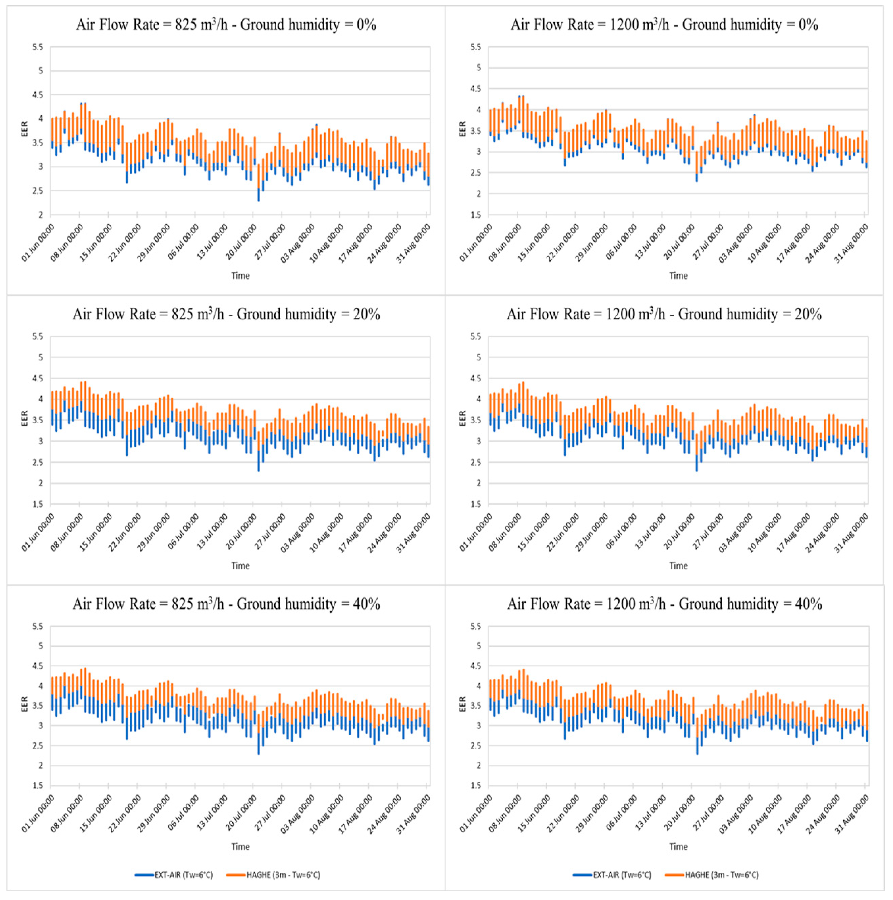
Figure 7 reports the EERs comparison for the whole period of summertime from 1 June to 31 August, for air flow rates of 825 m³/h and 1200 m³/h at burial depth of 3 m. The graphs show the trends comparison by two curves, blue for EER_EXT-AIR and orange for EER_HAGHE, by the variation of ground volumetric humidity 0–20–40%.

It is interesting to note that EERs with air treated by HAGHE are, on average, higher than ones with external air and seem to have smaller oscillations. Ground humidity seems to have a slow influence, varying between 20–40%.

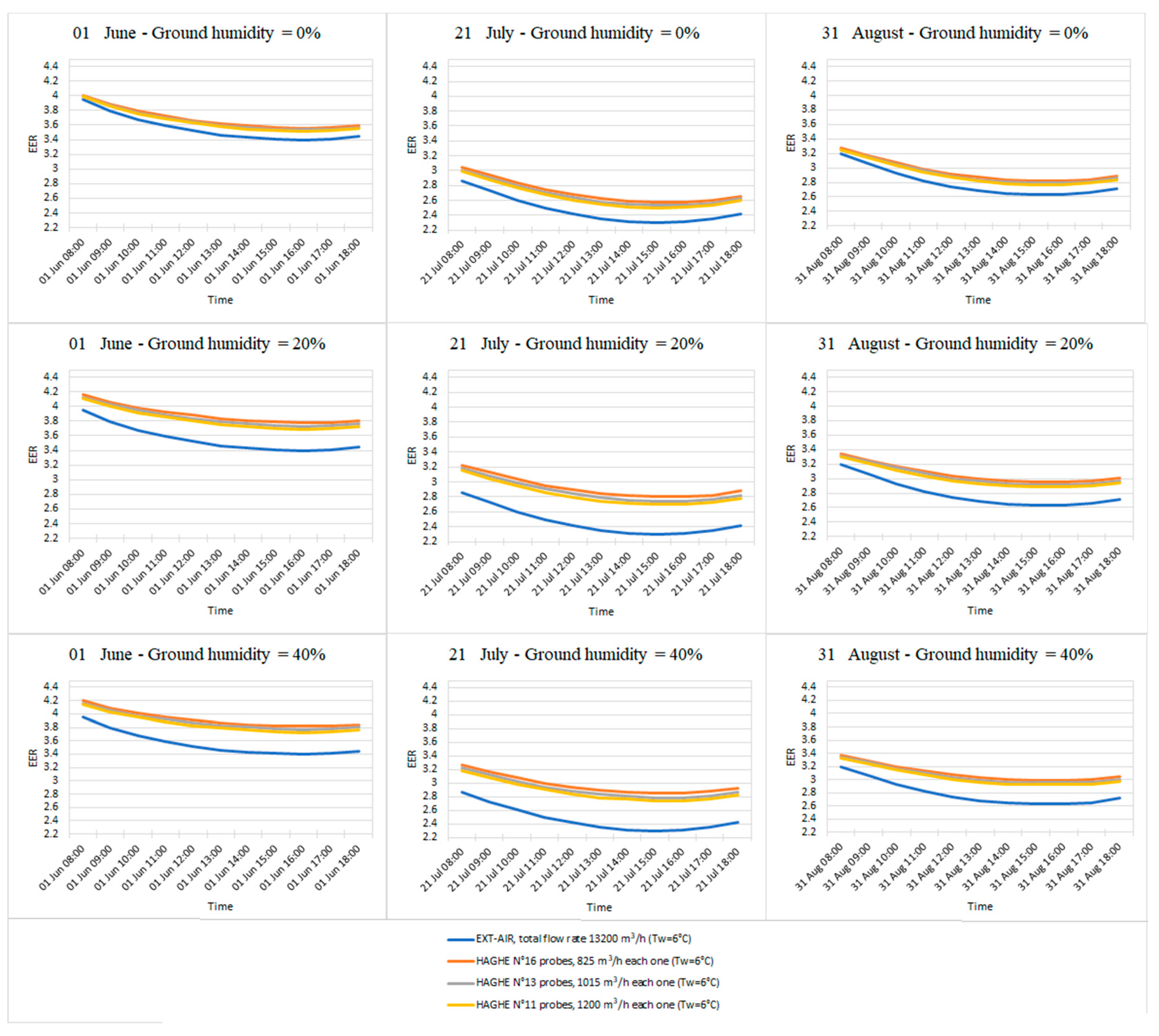
Figure 8 shows the comparisons for three selected days:

−

1 June (first day with air conditioning system turned on);

−

21 July (the warmest day);

−

31 August (last day, with air conditioning system turned on).

for the temperatures of the treated water by HAGHE of 6 °C, for the three flow rates selectedand and three ground volumetric humidity. The use of HAGHE affects the performance much more compared with the winter case. In all cases, passing from an air flow rate of 825 m³/h to 1200 m³/h, there is a small lowering of EER_HAGHE.

As regards 21 July shown in Figure 8, it is possible to observe a positive gap between the two curves EER_EXT-AIR and EER_HAGHE, but the mass flow rate shows a small influence on EER_HAGHE.

Ground volumetric humidity shows a great influence on the ACHP-HAGHE behaviour in summertime. The curves with ground volumetric humidity equal to 0% and 20%, are rather similar at the case with 40%, but the gap between EER_HAGHE and EER _EXT-AIR are slightly lower.

In numerical terms, the combination that returns the highest EER_HAGHE is characterized by a burial depth of 3 m, a 30 m probe length, an air flow rate equal to 825 m³/h, a ground water content of 40% for water temperature equal to 10 °C.

Like for COPs,

Table 6. Best values of EER (at T_w = 10 °C), L = 30 m, H = 3 m, G = 833.33 m³/h.

			Ground Volumetric Humidity = 0%	Ground Volumetric Humidity = 20%	Ground Volumetric Humidity = 40%
Date	Hour	EERAIR-EXT	EERHAGHE	EERHAGHE	EERHAGHE
1 June	8 a.m.	4.30	4.44	4.64	4.67
21 July	8 a.m.	3.12	3.33	3.54	3.60
31 August	8 a.m.	3.50	3.60	3.67	3.71

presents the highest values of the EER for the three ground volumetric humidities.

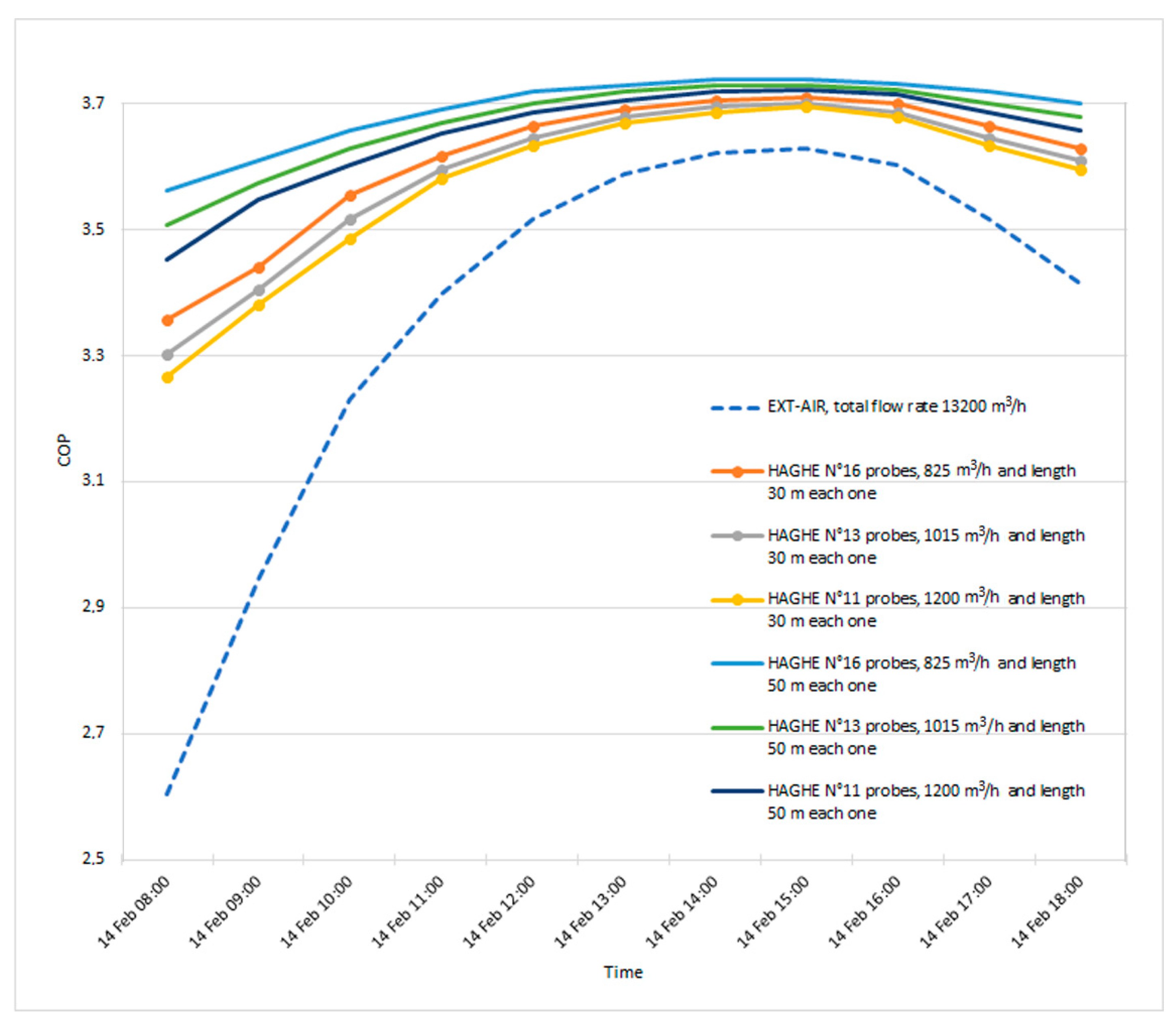
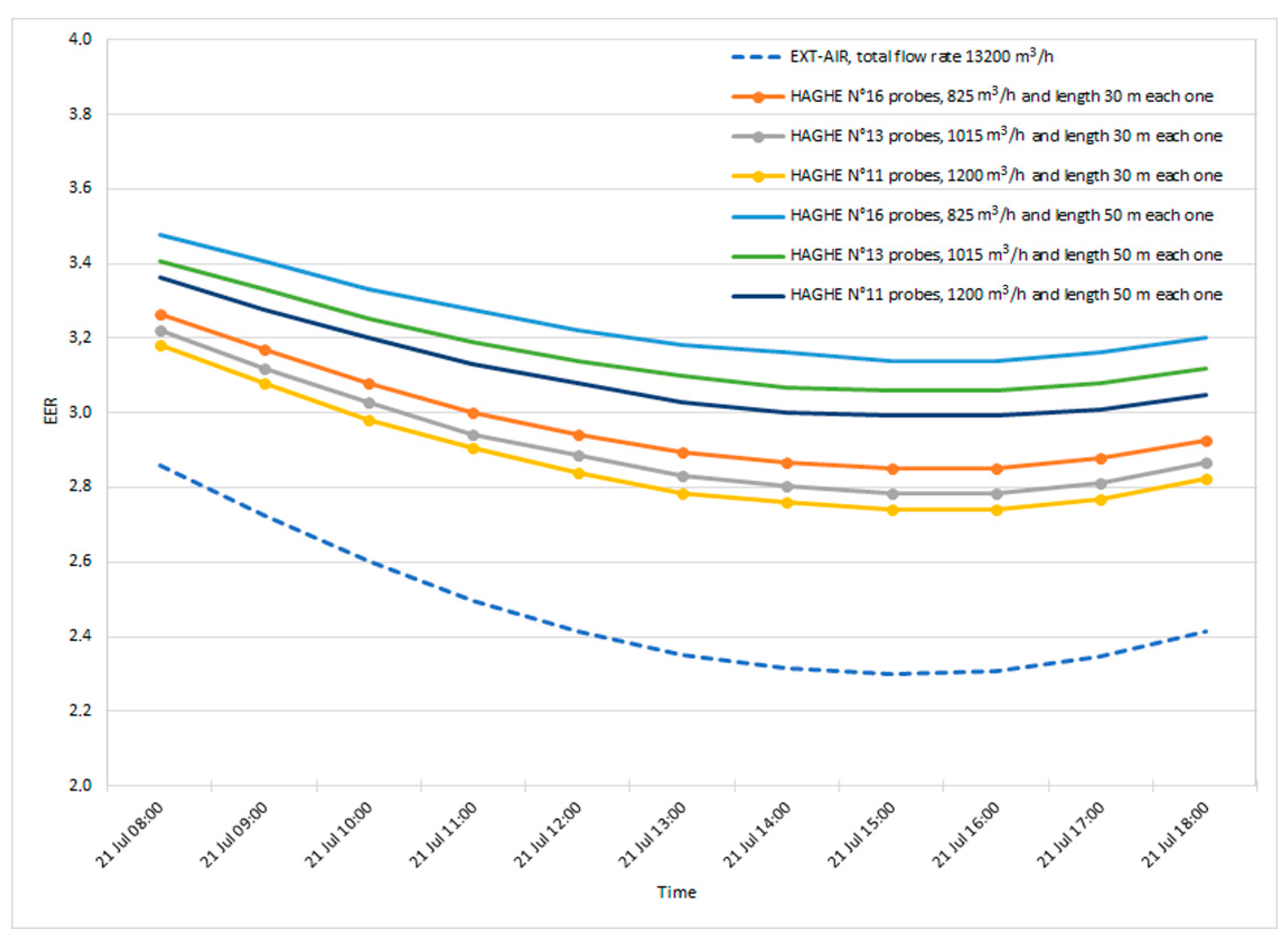
4.4. Evaluation of the Optimal Length of the Geothermal Probe

A comparison between 30 m and 50 m probe has been done. Figure 9 shows the comparison in the coldest day (14 February) between COP_EXT-AIR and COP_HAGHE by varying the air flow rate (825 m³/h, 1015 m³/h and 1200 m³/h) and the probe lengths (30 m and 50 m).

The EER comparison has been carried out for the warmest day of the year (21 July) in Figure 10.

Table 7. Hourly performance improvement (%) of COP respect of untreated case by varying probe length: 14th February, T_w = 35 °C, G = 833.33 m³/h, Ground humidity = 40%, H = 3 m.

Hour	COPEXT-AIR	COPHAGHE (30 m)	COPHAGHE (50 m)	Improvment % (L = 30 m)	Improvment % (L = 50 m)	∆50–30%
8	2.604	3.358	3.561	28.9%	36.7%	7.8%
9	2.944	3.441	3.610	16.9%	22.6%	5.7%
10	3.230	3.554	3.658	10.0%	13.3%	3.2%
11	3.398	3.616	3.690	6.4%	8.6%	2.2%
12	3.518	3.664	3.720	4.2%	5.7%	1.6%
13	3.589	3.690	3.729	2.8%	3.9%	1.1%
14	3.622	3.705	3.738	2.3%	3.2%	0.9%
15	3.628	3.710	3.738	2.3%	3.0%	0.8%
16	3.603	3.700	3.732	2.7%	3.6%	0.9%
17	3.518	3.664	3.720	4.2%	5.7%	1.6%
18	3.414	3.628	3.700	6.3%	8.4%	2.1%

and

Table 8. Hourly performance improvement (%) of EER respect of untreated case by varying probe length: 21 July, T_w = 6 °C, G = 833.33 m³/h, Ground humidity = 40%, H = 3 m.

Hour	EEREXT-AIR	EERHAGHE (30 m)	EERHAGHE (50 m)	Improvment % (L = 30 m)	Improvment % (L = 50 m)	∆50–30%
8	2.859	3.265	3.476	14.2%	21.6%	7.4%
9	2.724	3.171	3.408	16.4%	25.1%	8.7%
10	2.604	3.079	3.330	18.3%	27.9%	9.6%
11	2.496	3.001	3.276	20.2%	31.2%	11.0%
12	2.416	2.943	3.223	21.8%	33.4%	11.6%
13	2.353	2.896	3.181	23.1%	35.2%	12.1%
14	2.314	2.868	3.160	23.9%	36.6%	12.6%
15	2.299	2.850	3.140	24.0%	36.6%	12.6%
16	2.306	2.850	3.140	23.5%	36.1%	12.6%
17	2.345	2.877	3.160	22.7%	34.8%	12.1%
18	2.416	2.924	3.202	21.0%	32.5%	11.5%

highlight the percentage increase of the COP and EER, respectively. It is possible to note that the percentage increase of COP and EER by the use of the 50 m probe is not energetically significant to adopt its use. It suggests to use probes with a length of 30 m in parallel configuration rather than less probes longer because the last part of the probe works with lower temperature gaps.

4.5. Comparison of SCOPs

The SCOP_on is calculated to produce water at 35 °C (for radiant panels) and at 55 °C (for fan coils). As regard the SCOP_AIR-EXT, all the temperatures below 16 °C have been selected and the corresponding COPs have been included in the calculation; it has been supposed that, with an external air temperature over 16 °C, the air-conditioning system does not work. The calculation has been carried out with an hourly time step.

As regard the SCOP_HAGHE, the working periods of the air-conditioning system are the same of the case above, therefore in function the external air temperature (below or above 16 °C). The outlet air temperature from the probe is used for the calculation of hourly COP. Frequency of occurrence of outdoor air temperatures remain thus invariant for both cases.

Table 9. SCOP values with and without the use of geothermal probe (H = 3 m, L = 30 m, d = 0.5 m).

Tw (°C).	SCOP
	EXT-AIR	Air Flow Rate = 833.33 m3/h			Air Flow Rate = 1200 m3/h
		Ground Volumetric Humidity 0%	Ground Volumetric Humidity 20%	Ground Volumetric Humidity 40%	Ground Volumetric Humidity 0%	Ground Volumetric Humidity 20%	Ground Volumetric Humidity 40%
35 °C	2.91	2.98	3.03	3.04	2.96	3.01	3.02
55 °C	2.06	2.12	2.17	2.17	2.11	2.15	2.16

shows SCOP values calculated for the three ground volumetric humidity percentages (0–20–40%) and for two air flow rates (825 m³/h and 1200 m³/h) compared to the SCOPs of standard configuration. It is noted that the SCOP follows the same trend of the COP, it decreases with the increase of the ground volumetric humidity.

It is important to note that the SCOP is not much affected from the air mass flow rate. It suggests to use high mass flow rate to reduce the drilling cost. For example, for the air flow rate of 1200 m³/h, SCOP seems not influenced by the ground water content.

4.6. Comparison of SEERs

The SEER_on calculation is performed both to produce water at 6 °C and at 10 °C.

Table 10. SEER values with and without the use of geothermal probe (H = 3 m, L = 30 m, d = 0.5 m).

Tw (°C).	SEER
	EXT-AIR	Air Flow Rate = 833.33 m3/h			Air Flow Rate = 1200 m3/h
		Ground Volumetric Humidity 0%	Ground Volumetric Humidity 20%	Ground Volumetric Humidity 40%	Ground Volumetric Humidity 0%	Ground Volumetric Humidity 20%	Ground Volumetric Humidity 40%
6 °C	2.76	2.86	2.99	3.02	2.83	2.93	2.96
10 °C	3.03	3.15	3.29	3.33	3.12	3.23	3.26

shows SEER values calculated for the three ground volumetric humidity percentages (0–20–40%) and for two air flow rates (825 m³/h and 1200 m³/h) compared to the SEERs of standard configuration. It is noted that the SEER follows the same trend of EER and it decreases by the increasing of the ground volumetric humidity.

It is interesting to note that the coupling with HAGHE lets to improve the SEER for the whole cooling period, suggesting a better behaviour in the summertime respect to the wintertime in the Mediterranean climate.

5. Conclusions

The main goal of this paper is to show the increasing of the performance of an Air-Cooled Heat Pump (ACHP) coupled with a Horizontal Air-Ground Heat Exchanger (HAGHE). The innovation is to provide a geothermal treatment of pre-heating/cooling of air before meeting the evaporator and the condenser, in winter and summer, respectively.

The ACHP-HAGHE system has been investigated by varying parameters such as the length and the installation depth of the probe, the air flow rate and the ground thermal properties in terms of COP, EER and Seasonal Index as SCOP and SEER. The results show lower energy consumptions compared to a traditional Air-Cooled Heat Pump.

Regarding the winter, the results underline that, in warm climate, COPs show negligible improvement in the first and in the last fractions of the working period of the air-condition system. COPs show a good improvement during the coldest days of the winter.

Regarding the summer, the results underline that, in warm climate, EERs show a good improvement during the whole working period of the air-conditioning systems.

Finally, seasonal coefficients SCOP and SEER were calculated: in addition to the temperature at the inlet to the pump, they also take into account the frequency of occurrence of the temperature.

The SCOP values of ACHP-HAGHE system show a performance increase of 4.4% for the production of water at 35 °C and of 5.33% for the production of water at 55 °C.

As regards the SEER values, there is an increase in the performance of 9.4% for the production of water at 6 °C.

The best condition identified for the winter and summer period for Brindisi, in terms of COP, EER, SCOP and SEER, is a probe length equal to 30 m, the air inlet flow of 825 m³/h, burial depth of 3 m and thermal water content equal to 40%.

The proposed system shows several advantages respects to the traditional water geothermal heat pump. First of all, such a system permits to improve the performance of an existing air source heat pumps without its replacement.

Furthermore, the proposed system, using a bypass, allows heat pumps working always in the best condition. In winter, for example, working directly with the external air (without the geothermal probes) if its temperature is higher than the ground temperature or, if lower, with the geothermal probes; vice versa in summer.

This solution can also be useful for not exploiting the ground when it is saturated due to long use and avoids the system stopping.

The geothermal probes can be easily converted in a free-cooling ventilation system using a bypass in the middle seasons when the heat pump does not work.

Typically, the traditional water geothermal heat pump needs to use glycol mixed with water to prevent freezing, this fluid can be dangerous and lead to related problems of disposal.

The estimated cost of excavation, probes installation and backfilling of the soil is about € 1800/2000 for a probe with a length of 30 m. This cost may be reduced in the construction phase of the building.

The annual electrical consumption for ACHP is about 16,700 kWh without the use of HAGHE system and 15,585 kWh with the use of geothermal probes. The energy saving is about 1115 kWh.

The future development could be the cost-optimal analysis of the system considering also the passive cooling of the building through night-time free cooling.