The Spatial Network Structure of China’s Regional Carbon Emissions and Its Network Effect

1
School of Management, China University of Mining and Technology, No. 1, College Rd., Tongshan Dist., Xuzhou 221116, Jiangsu, China
2
Program on Chinese Cities, University of North Carolina at Chapel Hill, 314 New East Building, CB 3140, Chapel Hill, NC 27599-3140, USA
*
Author to whom correspondence should be addressed.
Energies 2018, 11(10), 2706; https://0-doi-org.brum.beds.ac.uk/10.3390/en11102706
Submission received: 7 September 2018
/
Revised: 30 September 2018
/
Accepted: 4 October 2018
/
Published: 11 October 2018
(This article belongs to the Section L: Energy Sources)
Abstract
:Under the “new normal”, China is facing more severe carbon emissions reduction targets. This paper estimates the carbon emission data of various provinces in China from 2008 to 2014, constructs a revised gravity model, and analyzes the network structure and effects of carbon emissions in various provinces by using social network analysis (SNA) and quadratic assignment procedure (QAP) analysis methods. The conclusions show that there are obvious spatial correlations between China’s provinces and regions in terms of carbon emissions: Tianjin, Shanghai, Zhejiang, Jiangsu and Guangdong are in the center of the carbon emission network, and play the role of “bridges”. Carbon emissions can be divided into four blocks: “bidirectional spillover block”, “net beneficial block”, “net spillover block” and “broker block”. The differences in the energy consumption, economic level and geographical location of the provinces have a significant impact on the spatial correlation relationship of carbon emissions. Finally, the improvement of the robustness of the overall network structure and the promotion of individual network centrality can significantly reduce the intensity of carbon emissions.
1. Introduction
With the rapid development of China’s economy, environmental pollution problems have intensified. Carbon dioxide is the main greenhouse gas present in the atmosphere. Its excessive emission will exert pressure on the ecological environment and will not be conducive to sustainable economic development [1]. According to the 2007 carbon emissions statistics, China’s carbon emissions have surpassed those of the United States to become the world’s largest carbon emitter [2]. In 2015, China proposed positive national independent contribution targets at the Paris Climate Conference. These targets include: CO2 emissions peak around 2030 and non-fossil energy accounts for about 20% of primary energy; in 2030, CO2 per unit of GDP decreased by 60–65% compared with 2005 [3]. However, due to the combination of economic level, geographical location and industrial structure, carbon emissions in various regions of China show uneven spatial characteristics [4,5]. Therefore, the overall understanding of the spatial relationship between carbon emissions and the inter-regional carbon emissions-associated network structure is a guarantee for achieving regional carbon synergy emissions reduction targets.
From the perspective of spatial analysis, the existing research mainly examines the spatial distribution, spatial dependence and transfer relationship of carbon emissions between different regions. Scholars mainly use the indicators of the Theil index, Gini coefficient and Esteban-Ray index to measure the spatial difference of carbon emissions among different countries and regions. Research shows that energy structure, energy intensity and other factors are the main factors causing spatial differences in carbon emissions [6]. At the same time, many scholars have gradually found that carbon emissions have significant spatial dependence characteristics [7,8]. The spatial differences in carbon emissions and the objective existence of spatial dependence have prompted the spatial transfer of carbon emissions to become a new research hotspot [9,10,11]. However, most studies only limit spatial correlation to “adjacent” or “close” regions, and generally ignore the impact of the relationship between carbon emissions entities on carbon emissions. From the perspective of research methods, some studies use social network analysis (SNA) to explore regional spatial network research [12,13]. Most of the research on carbon emissions focuses on carbon emission measurement and decomposition, carbon emissions influencing factors and carbon emissions reduction measures [14,15,16,17], and some scholars have studied the carbon emissions trading market [18]; despite there being also spatial network research on carbon emissions in China, the scope of the research only covers some areas [19], and the research granularity is small, making the spatial network of research relatively shallow.
In recent years, there has been considerable research literature on the spatial correlation of carbon emissions in China. More and more researchers have proved that carbon emissions do not exist independently in various regions but in a certain spatial correlation. Wu Yuming empirically analyzed the spatial effects and drivers of China’s provincial carbon emissions using a spatial econometric model [20]; Zhang Degang and Lu Yuanquan used social network analysis methods to deconstruct the spatial correlation characteristics of China’s carbon emissions, based on quadratic assignment procedure (QAP) technology, and reveal the main influencing factors of carbon emissions spatial correlation [21]; Du Qiang et al. used Shanxi province of China as an example to study the spatial correlation network characteristics of carbon emission in industrial sectors [22]; Zhou Yingying and Sun Yuyu constructed a spatial correlation network of carbon emissions in the Yangtze River Economic Belt by integrating geographical distance, economic level, population size, carbon emissions, etc., and studied the characteristics of network structure through social network analysis [23]. Existing research often considers the spatial correlation of carbon emissions from the perspective of provinces or regions, and this research is slightly weak in terms of low-carbon spatial networks in provinces and regions across the country.
Compared with the existing literature, the main innovation of this paper is to use the SNA method and the QAP method to explore the spatial correlation and network effect of regional carbon emissions from the perspective of complex networks. When using traditional spatial measurement methods to analyze carbon emissions and their influencing factors, most of the literature only considers geographically similar factors [22,23]. At the same time, since the “Twelfth Five-Year Plan”, China has established a carbon emissions trading market as an important task. The establishment of this market will promote the spatial correlation of carbon emissions to a certain extent. This paper attempts to use social network analysis to explore the network association law of carbon emissions between different provinces. This attemption will helps us understand the spatial correlation characteristics of China’s regional carbon emissions more comprehensively, especially when the spatial correlation characteristics are very significance for the carbon emissions control based on the combined effect of different regions.
2. Methodology and Data
2.1. Determination of the Spatial Correlation Network of Carbon Emissions
In this paper, the carbon emission data of each province in China is taken as the network node. The “line” between the two nodes in the associated network is defined as the spatial correlation between the provinces in terms of carbon emissions, and thus constitutes the spatial correlation network between the provinces in terms of carbon emissions. There are mainly gravitational models and VAR (Vector Autoregression Model), one is based on the Granger Causality test method, such as Li Jing [24], Liu Huajun [25], etc. The other is based on the gravity model or the improved gravity model, such as Hou Yuhui [26] and Liu Huajun [27] models for constructing spatial correlation networks. This paper selects the gravitational model to describe the spatial correlation between carbon emissions in various regions. The two reasons are as follows: first, the gravity model, which is more suitable for aggregate data, can integrate geographic distance, economic level, population size and other factors portraying the strength of the relationship between two regions. Second, the gravity model involves fewer factors and easily collected data, making it more suitable for the measurement of inter-regional gravity. This paper corrects the original formula, and applies the gravity model of regional economic linkage quantitative analysis to the spatial correlation of carbon emissions in various provinces of China. The modified gravity model is as follows:
where: i and j indicate the provinces i and j, respectively; xij indicates the gravity between provinces i and j; Pi and Pj indicate the total population of provinces i and j; Ci and Cj indicate the carbon emissions of the two different provinces; Gi and Gj indicate the actual regions of provinces i and j’s gross production value; Dij indicates the geographical distance between provinces i and j; and gi − gj indicates the difference in GDP per capita between provinces i and j. According to Formula (1), the gravitational matrix between the provinces is obtained, and each row of the gravitational matrix is averaged; then, the average value is compared with the row data in the matrix, and if it is greater than the mean of each row, it is recorded as 1, indicating that the province in which the row is located is associated with carbon emissions in the province in which the column is located, and that the line draws a direct line to the column. Otherwise, it is marked as 0, indicating that there is no correlation. This creates a spatially correlated network matrix of carbon emissions across provinces.
2.2. Characteristics of China’s Provincial Spatial Correlation Network of Carbon Emissions
2.2.1. Overall Network Characteristics
The first index, which describes the characteristics of the overall network, is the network correlation degree the network correlation degree is an indicator reflecting the tightness of the spatial correlation network of carbon emissions. In the carbon emission-related network, if there are more direct or indirect connections between any two nodes, the stability of the associated network will be better, otherwise the network is more vulnerable. The network density is the closeness of the relationship between any two nodes in the carbon emission network. If the network density is higher, the two provinces represented by the two nodes are related to carbon emissions closely. The network efficiency is the degree of the efficiency of linkages between nodes in a carbon emission network. The network level reflects the position of each node member in the overall network.
2.2.2. Network Characteristics of Each Node
The closeness centrality indicator can be used, first, for characterization in the carbon emission-related network. The closeness centrality reflects to the degree showing each node is not controlled by other nodes in the overall carbon emissions network. The second is the betweenness centrality, which refers to the degree to which a node can control the relationship between other nodes. The higher the betweenness centrality of a province is, the more control the province can have for the interaction between other provinces in carbon emissions. In addition, the degree of point centrality which reflects the degree of the central position of the provinces in the spatial association network. If the province’s degree of point centrality is higher, the province is at the center of the overall carbon emissions network.
2.2.3. Block Model Analysis
Block model analysis is a common analysis method in social network analysis, originally proposed by Boorman and White [28] and Smith and White [29]. The Cassi [30] block model is mainly used to analyze the location of each node in the overall network. The block model analysis is more intuitive for examining the development status inside the carbon emissions spatial correlation network and for a more comprehensive understanding of the complex links between the various blocks. In this article, the carbon emissions spatial correlation network is divided into four types according to the evaluation model of Wasserman and Faust [31]. The first block is the net beneficial block, in which the network members can not only receive the relationship between the members of other network members, but also between the members of the internal network of the block. The external relationship between the received blocks is obviously more than any block’s overflow relationship with other blocks. The second block is the net spillover block, which, like the above, sends more information to other blocks than it receives, and therefore it is also a bidirectional spillover block. The block sends information to other blocks while receiving information from other blocks. The information of the network members that the block received is also relatively large. The last block is the broker block, which sends out information and receives information between other blocks; the connection between this type of block and other block network members is more complicated.
2.3. Data
In this paper, 30 provinces in China are used as network nodes (Hong Kong, Macao and Taiwan and Tibet’s data are missing), and the sample period is from the years 2008 to 2014. The gravitational model measures, the data sources and their treatments are as follows: carbon emissions are measured by Intergovernmental Panel on Climate Change (IPCC) (2006); the population and GDP data of each province are derived from the corresponding year’s China Statistical Yearbook, and the GDP of each province is converted to the true value of the base period in 2008, with the GDP deflator of each province; the geographical distance between the provinces is represented by the spherical distance between the provincial capitals.
3. Results and Discussion
3.1. Structural Characteristics of Spatial Correlation Networks for Carbon Emissions in China’s Provinces
3.1.1. Analysis of Overall Network Characteristics
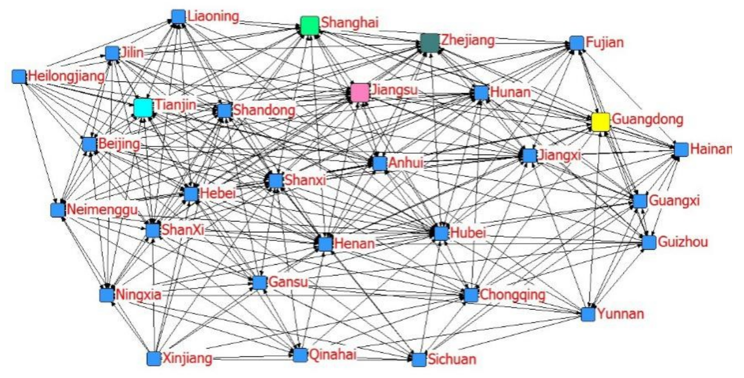
According to Equation (1), the carbon emission spatial correlation matrix constructed by the gravity model is based on the data of 30 provinces in China for the year 2014. Using the Netdraw visualization tool in UCINET software (UCINET v6.0, Analytic Technologies, Lexington, KY, USA), the network correlation diagram of carbon emissions in each province is drawn. It can be clearly seen from Figure 1 that there is a significant spatial network correlation between carbon emissions in each province, and it can be observed that the network shape is stable with typical network structure characteristics [32,33]
(1) Network density and association relationship
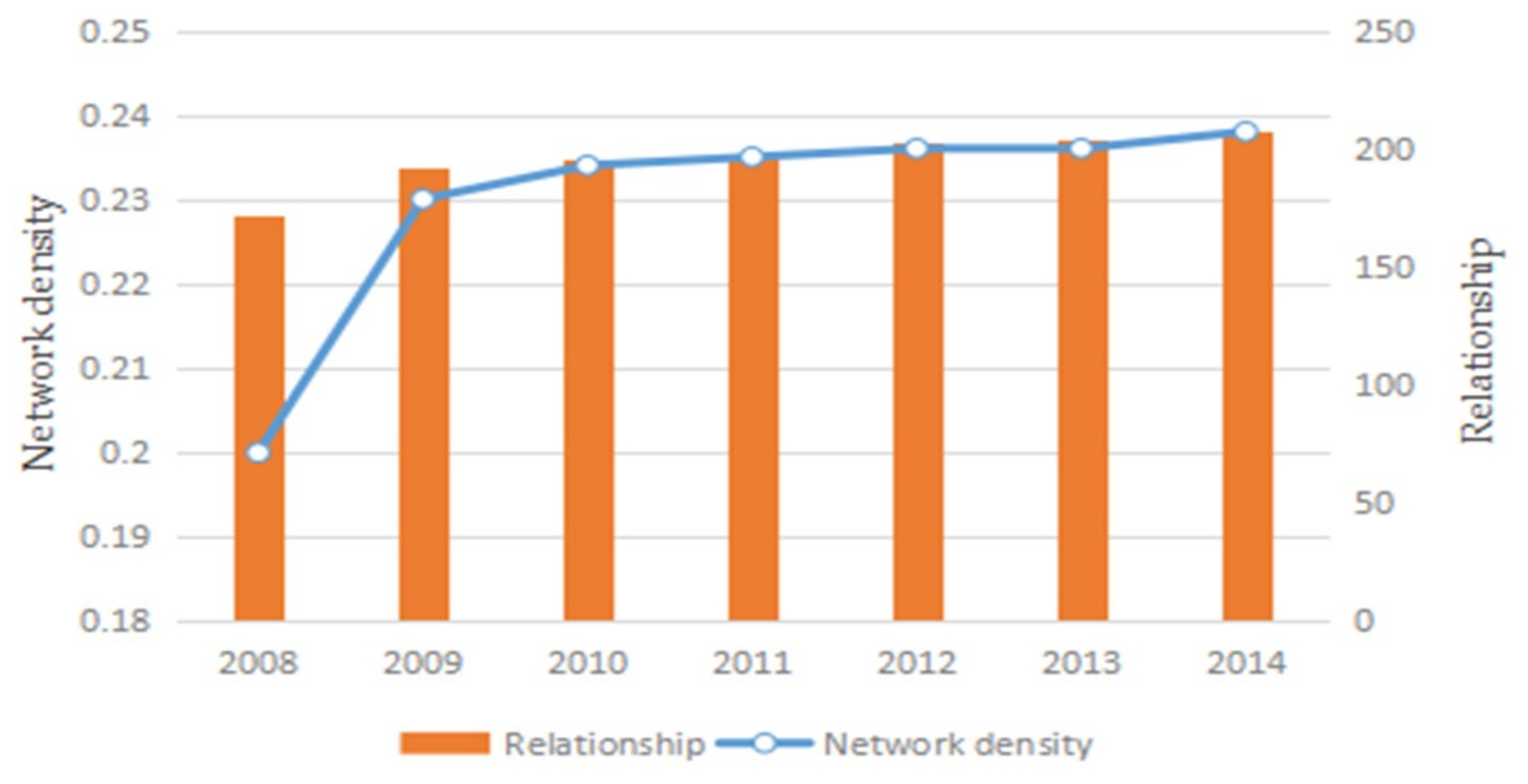
The following can be seen from Figure 2: In the carbon emission related network, the number of network relationships shows an upward trend in the sample period, from 166 in 2008 to 208 in 2014, reaching 201 in 2010. After 2010, the number of network relationships gradually tends towards a stable stage. At the same time, the network density during the sample period gradually increased from 0.2 in 2008 to 0.239 in 2014. Obviously, in the period from 2008 to 2014, the spatial correlation of carbon emissions in various provinces became higher and higher. The reasons may be related to the accumulation of various industries and the division of energy regions in recent years. The agglomeration of various industries and the cross-regional flow of energy will inevitably promote the spatial correlation of carbon emissions in various provinces.
Although the network density and the number of network associations in the sample period are gradually increasing, there is still a big gap between the largest possible network association numbers. Thus, China has a lot of space to promote the spatial correlation of carbon emissions [34].
(2) Network level and network efficiency
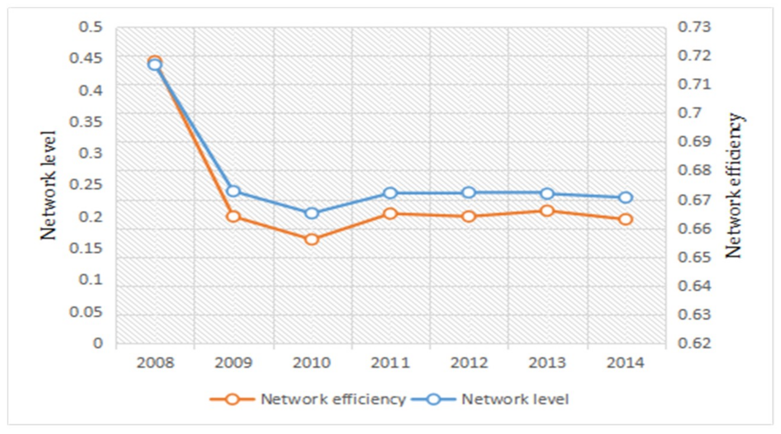
The degree of network correlation can reflect the correlation of a network in terms of carbon emissions. During the period from 2008 to 2014, the annual network correlation degree is 1, and therefore an obvious spatial correlation effect of carbon emissions exists between the provinces. It can be seen from Figure 3 that the overall network level and network efficiency during 2008 to 2014 are in a downward trend, indicating that there is no strict hierarchical phenomenon in terms of carbon emissions between provinces, that there is a close relationship among the provinces in the carbon emission network, and that the network structure is becoming more and more stable.
Based on the above analysis, with the advancement of China’s modernization and marketization, China’s energy market is constantly improving, and industrial production is developing too. This also means that carbon emissions are distributed closely in space and stabilized gradually. With the establishment and improvement of China’s carbon emissions trading market, this connection will gradually increase [18].
3.1.2. Central Analysis
The central analysis of carbon emissions in China’s provinces in 2014 is shown in Table 1, this analysis is consistent with the research findings of previous researchers [21]. It proves that the five provinces thar have the highest degree of point centrality in all relationships are Shanghai, Jiangsu, Zhejiang, Guangdong, Tianjin, and Guangdong. Considering that the regions with those provinces are economically developed and have more connections with other provinces involved in industrial development, those provinces are actually located in the center of the carbon emissions related network, such as the Yangtze River Delta, the Pearl River Delta and the coastal areas. In that case those provinces have a greater degree of benefit and weaker self-sufficiency, which means less spillover. Considering that the number of associations in each province includes both the number of relationships sent and received, the top five provinces with the receiving and sending relationships are analyzed: Shanghai, Jiangsu, Zhejiang, Guangdong and, Tianjin. Compared with previous studies [21], the number of receiving relationships in Jiangsu province increased significantly. The top five provinces with the highest sending relationships are Shanghai, Guangdong, Qinghai, Gansu, and Xinjiang, all of which are located in the eastern region. The top five provinces with the highest transmission relationship, except Guangdong and Shanghai, are located in the western region, indicating that the western region mainly has spillovers, while the eastern region mainly has benefits in the spatial network of carbon emissions. This conclusion is similar to the past. In the regions with the highest degree of point centrality, Shanghai, Tianjin, Guangdong (including Shenzhen) were the pilot areas in China to allow carbon emissions trading in 2012, but all of the carbon markets started trading in 2013, and the trading volumes were small. With the reason that Shanghai, Jiangsu, Zhejiang, Guangdong and Tianjin have positions of importance, the roles of these provinces in the carbon spatial network are further demonstrated.
3.1.3. Block Model Analysis
The block model is analyzed by using the CONCOR (convergent correlation) iteration method in UCINET software, with a convergence index of 0.2 and a maximum segmentation of 2. The analysis results are shown in Table 2. China’s 30 provinces were divided into four blocks [34] as follows: the first block includes three provinces—Beijing, Neimenggu and Liaoning; the second block includes eight provinces—Shanghai, Jiangsu, Zhejiang, Guangdong, Tianjin, Fujian, Anhui and Shandong; the third block includes 10 provinces—Jilin, Heilongjiang, Hebei, Ningxia, Henan, Gansu, Qinghai, Shanxi, Xinjiang, Shanxi; and the fourth block includes nine provinces—Hunan, Chongqing, Guizhou, Yunnan, Hubei, Guangxi, Hainan, Jiangxi, and Sichuan
The numbers of transmission and reception relationships outside the plate of the first block are 19 and 15, respectively, and the actual relationship ratio inside the block is 11.76%, which is greater than the expected internal ratio of 6.90%. At the same time, there is an overflow relationship between the inside and outside of the block, so this belongs to the “bidirectional spillover block”; the number of receiving relationships in the second block is 118, and the number of relations issued is 57. The actual internal relationship ratio is 52.63%, which is greater than the expected internal relationship ratio of 24.14%, and the number of receiving relationships outside the second block is 88, which is much larger than the number of external relations—19—received by the first block, so the second block belongs to the “net beneficial block”. The reason for this is that most of the provinces in the second block are located in the more developed urban agglomerations such as the Yangtze River Delta, the Pearl River Delta and the coastal areas. Due to poor resource endowment and weak self-sufficiency, these are in the “net beneficial block”; the number of receiving relationships in the third block is 23, and the number of relations issued is 73. The number of relations issued outside the block is 69, which is higher than the number of external relations, 46, issued by the fourth block. Therefore, the net spillover effect on carbon emissions is large. At the same time, the ratio of internal relations is expected to be 31.03%, which is less than the actual internal relationship ratio of 5.48%. Therefore, the third block belongs to the “net spillover block”. The reason is that most of these provinces belong to remote areas in the west and are strongly self-sufficient, and so most of the energy shows a spillover effect; in the fourth block, the total number of received relationships is 29, and the total number of issued relationships is 54. The expected internal relationship ratio is 27.59%, which is larger than the actual internal relationship ratio of 14.81%. These provinces have more receiving relationships and issue relationships. There are also many numbers, and so the fourth block belongs to the “broker block”; there are more links with other blocks, but the links between the internal blocks are relatively small. Consistent with previous studies, the third and fourth blocks are rich in coal, oil and natural gas, providing abundant energy resources for the Beijing–Tianjin–Hebei, Yangtze River Delta and Pearl River Delta [34], but the differences exist in the sector-related networks, the carbon loss of the first block to the third block and the second plate to the fourth block overflows, which indicate that each segment play a “comparative advantage” in the carbon emission-related network, and the linkage effect of the “national chess game” becomes more and more obvious.
3.2. Analysis of the Influence Factors of the Spatial Correlation of Carbon Emissions in Provinces Based on the Quadratic Assignment Procedure (QAP) Analysis Method
3.2.1. Model Construction
After analyzing the spatial correlation characteristics of carbon emissions in all provinces of China, this paper explores the factors that influence the spatial correlation of carbon emissions. Many studies have shown that the spatial spillover effects of corresponding carbon emissions are different in different geographical positions and are to some extent affected by adjacent areas [34]; thus, the proximity of geographical position is an important factor affecting the spatial correlation of carbon emissions. According to the results of the block model analysis above, there are more spillover relationships between the developed regions in the east and the undeveloped regions in the west, and so the spatial correlation of carbon emissions is related to the regional level of economic development. Therefore, the selection of the energy structure, industrial structure, opening level and economic level index indirectly depict the comprehensive development differences of each region. The corresponding observational indexes are as follows: the proportion of coal consumption to total energy consumption (C), the proportion of added value of secondary industry and tertiary industry (I), gross import and exports/GDP (E), and per capita GDP (P). Based on the above analysis, it is theoretically possible to set the model as S = f(G,C,I,E,P), where S is the spatial correlation matrix of carbon emissions in all the provinces of China, 2014; G is the geographical proximity matrix, which is represented by the actual distance between the two provinces (the distance between the two provincial capitals), and then the mean value of each row is compared with the its element, if it is greater than the mean value as 0, otherwise as 1; the energy structure difference matrix, C; the industrial structure difference matrix, I; the difference matrix of the level of opening to the outside world, E; and the economic level difference matrix, P, respectively, use the absolute difference of the corresponding index of various provinces and cities in 2014 to construct the difference matrix. In the empirical process the regression variables are the relationship matrix representing the two regions and, therefore, compared with previous studies [34], it is not possible to use general methods to test whether there is a relationship between variables, and we should choose the common method of social networks: the QAP regression analysis method [34]. This method can better deal with the problem of overlap between independent variables in regression.
3.2.2. QAP Regression Analysis
QAP regression is used to study the regression relationship between a matrix and multiple matrices. There are two specific implementation steps: firstly, the regression analysis of the corresponding elements of the independent variable matrix and the dependent variable matrix; the random permutation of each row and column of the dependent variable matrix and the regression are recalculated, and all coefficient values and decision coefficient values recorded. In this paper, the results of a permutation performed 2000 times and QAP regression analysis are shown in Table 3. Probabilities 1 and 2, respectively, represent the probability that the regression coefficient is greater-or-equal or lesser-or-equal to the final regression coefficient in the process of random substitution.
Table 3 shows that the regression coefficients of spatial proximity matrix G, determined by geographical location, and per capita GDP difference matrix P, determined by economic level, are significant at the level of 1%, indicating that geographical position and economic development level have an important impact on the carbon emissions of provinces and regions in China; the regression coefficient of the energy structure difference matrix C, which takes coal consumption as the proportion of total energy consumption, is also significant at 5%. This shows that the energy consumption between provinces also has a significant impact on the carbon emission spillover, while the negative regression coefficient indicates that the greater the similarity of energy consumption in each region, the greater the spatial spillover effect of carbon emissions; the regression coefficient of the industrial structure difference matrix I is significant at the 10% level, which shows that the different industrial structure in each province will reduce the spatial spillover of carbon emissions to some extent. The negative regression coefficient of the level of opening to the outside world of difference matrix E shows that the higher the level of opening to the outside world, the more the spillover effect of carbon emissions will be reduced to some extent.
It can be seen from the normalized regression coefficients in Table 3 that the absolute value of regression coefficients of the geographical proximity difference matrix, the energy consumption difference matrix and the economic level difference matrix are large, which shows that the spatial relationship of carbon emissions is most affected by the geographical position factor and energy consumption difference as well as the economic level difference between the provinces [34].
3.3. Network Effects of Spatial Correlation of Carbon Emissions in China’s Provinces
After depicting the network characteristics of the spatial correlation of carbon emissions in China’s provinces and its influencing factors, the network effect of the spatial correlation of carbon emission is further studied.
In this paper, the carbon emission intensity of each province is interpreted as a variable; according to the degree of point centrality, betweenness centrality and closeness centrality of each province, the panel data is analyzed by regression analysis [27], the results of the Hausman test are given, and the regression coefficients of the three regression models can be seen as negative from Table 4; this is different from previous studies [27], and shows that three values of degree of point centrality, betweenness centrality and closeness centrality can effectively reduce carbon emission intensity in the carbon emission spatial correlation network.
Based on the estimated results of Table 4, the following can be observed:
- (1)
- The degree of point centrality coefficient is −0.008, indicating that for each unit of the point of centrality value, the carbon emission intensity decreases by 0.004 units. In Qinghai, Ningxia, Guangxi, Shaanxi, Jilin and other provinces, degree centrality is small, meaning that they can be strengthened with the neighboring provinces of carbon emission links to better promote the effective reduction of carbon emission intensity.
- (2)
- The betweenness centrality coefficient is −0.004, indicating that for each unit of the betweenness centrality value, the carbon emission intensity decreases by 0.004 units. In Shanghai, Jiangsu, Zhejiang, Guangdong, Fujian and other provinces, the betweenness centrality is higher. Most of these regions are located in the Yangtze River Delta and Pearl River Delta urban agglomeration, which are within the “hub” status in the overall network structure, and have a strong spatial spillover effect on carbon emissions in other provinces, effectively promoting overall carbon emission intensity reduction;
- (3)
- The closeness centrality of the regression coefficient value is −0.007, indicating that for each unit of the closeness centrality value, the carbon emission intensity decreases by 0.007 units. The higher the closeness degree, the closer the linkages in the overall network structure of the provinces are. Ningxia, Xinjiang, Qinghai, Jilin and other provinces with lower close closeness degrees can strengthen the connection with provinces in the center of the network, which can be effective to reduce carbon intensity.
4. Conclusions and Policy Implications
According to the carbon emission data of various provinces of China from 2008 to 2014, the spatial correlation matrix of carbon emission in each province is constructed according to the modified gravitational model. The network correlation diagram is drawn. At the same time, the structure and network effects of China’s provincial carbon emission correlation network are analyzed by using the social network analysis method. The main results indicate the following:
- (1)
- There are obvious spatial correlations between China’s provinces and regions in terms of carbon emissions. During 2008 to 2014, the network density increased by 19%, the network efficiency decreased by 7.66%, the network level decreased by 47.7%, and the network correlation degree was always 1, which indicates that the spatial correlation network structure of carbon emissions in China’s provinces has gradually stabilized.
- (2)
- The degree of point centralities of the five developed areas, including Shanghai, Tianjin, Zhejiang, Jiangsu and Guangdong provinces, is at the top. Those provinces are in the center of the carbon emissions network, and have more relations of reception. But in Gansu, Ningxia, Xinjiang, Heilongjiang, Qinghai, Jilin and other remote underdeveloped areas in the west, the degree of point centrality ranking has been lower but with more divergent relations, while most other provinces act as hubs. In the regions with the highest degree of point centrality, Shanghai, Tianjin, Guangdong (including Shenzhen) were the pilot areas in China to allow carbon emissions trading in 2012, but all of the carbon markets started trading in 2013, and the trading volumes were small. However, Shanghai, Tianjin and Guangdong are all economically developed regions, Jiangsu and Zhejiang are always the top economically developed provinces, and all of these five regions belong to the coastal areas in China. Whereas, the regions with low-ranking degree of point centrality are inland regions with relatively low level of economic development in China. Therefore, we believe that the reason for this result may be related to the level of regional economic development and their geographical location.
- (3)
- Carbon emissions can be divided into four blocks: “bidirectional spillover block”, “net beneficial block”, “net spillover block” and “broker block”.
- (4)
- The differences in the energy consumption, economic level and geographical location of the provinces have a significant impact on the spatial correlation relationship of carbon emissions.
The above conclusions indicate that China’s provinces have complex spatial correlations in terms of carbon emissions [31,32]. It is difficult to achieve a long-term mechanism for carbon emissions reduction by relying solely on the carbon emissions reduction targets of the provinces.
According to the conclusions of this paper, the following suggestions are put forward:
- (1)
- According to the structure and characteristics of the spatial network of carbon emissions in China, we should better understand the flow mechanism of carbon emissions and its conductivity, allocate carbon emission indicators across regions, and fully realize the coordinated emission reduction plan. With the establishment and improvement of China’s carbon emission trading market [18], the correlation of carbon emissions among the provinces has also increased year by year. Therefore, in the formulation of emission reduction plans, it is necessary to fully consider the relationship between the regions, and to solve the problem of optimal allocation of carbon emission from the micro and macro levels. Economically developed regions such as Beijing, Shanghai, and Tianjin are in the center of the network, and these provinces have high dependence on carbon emissions in resource-rich regions such as Xinjiang and Shanxi, reflecting the higher demand for carbon emissions in these economically developed regions. Therefore, it is possible that by establishing a “satellite” industrial chain through high carbon emission transfer can solve the problem of high carbon emissions in some regions. The Jiangsu, Zhejiang and Shanghai regions are “net beneficial” blocks with large populations, dense industry and huge carbon emissions, and these regions can also use industrial transfer methods to solve high carbon emissions. For the “net spillover” blocks in resource-rich areas, which have low economic development and low demand for carbon emissions, we can introduce high-carbon industries from developed regions, and balance the problem of excessive carbon emissions in some regions. Some mid-western regions are “brokers” blocks, which are closely linked to other sectors, and these regions should maintain a “middleman” role in allowing carbon emissions to be transmitted and flow through the network.
- (2)
- Continuously optimize China’s carbon emission spatial network, gradually reach the regional carbon emission balance, and achieve balanced emission reduction. We think that the implementation of different regional environmental policies may have a positive effect on reducing regional carbon emissions leakage, especially in non-power industries. In view of the characteristics of direct spillover in the eastern part of China and indirect spillovers in the western region, a corresponding carbon emission reduction policy was formulated to comprehensively consider both energy transfer costs and industrial transfer costs when implementing the “Southern Coal North Transportation” as well as “Western Gas East Transportation” on energy. Cost: not only will this consideration ensure the energy and carbon emissions of coastal economy developed regions, but also enables consideration of the ecological and economic costs brought about by high carbon emission.
- (3)
- Achieve balance and fairness between carbon emissions in all provinces across the country. According to the results of QAP regression analysis, the differences in energy consumption, economic level and geographical location between provinces have a significant impact on the spatial relationship of carbon emissions, and the adjacent carbon emission in the regions are obviously overflowing. Therefore, it is necessary to continuously narrow the economy and energy consumption differences between regions from the perspective of comprehensive development. The above conclusion can be realized through inter-regional low-carbon technology exchange, industrial transfer and population planning, and so can continuously improve China’s carbon emissions spatial network.
Author Contributions
F.W. and M.G. conceived and designed the experiments; M.G. performed the experiments; F.W. analyzed the data; and F.W., J.L. wrote the paper. All the authors read and confirmed the final manuscript.
Funding
This research was funded by [National Natural Science Foundation of China] grant number [71673270; 71403268; 71874185], and [China Scholarship Council Project] grant number [201806425016].
Acknowledgments
This work was supported by the National Natural Science Foundation of China (Grant No. 71673270; No. 71403268; No. 71874185), and China Scholarship Council Project (Grant No. 201806425016).
Conflicts of Interest
The authors declare no conflict of interest.
References
- Zafeiriou, E.; Arabatzis, G.; Tampakis, S.; Soutsas, K. The impact of energy prices on the volatility of ethanol prices and the role of gasoline emissions. Renew. Sustain. Energy Rev. 2014, 33, 87–95. [Google Scholar] [CrossRef]
- Dong, F.; Yu, B.; Hadachin, T.; Dai, Y.; Wang, Y. Drivers of carbon emission intensity change in China. Resour. Conserv. Recycl. 2018, 129, 187–201. [Google Scholar] [CrossRef]
- Ding, J. Paris Climate Change Conference and China’s Contributions. Public Dipl. Q. 2016, 1, 41–47. [Google Scholar]
- Yang, Q.; Liu, H. Regional Disparity Decomposition and Influencing Factors of Carbon Dioxide Emissions in China—Based on the Research of Provincial Panel Data from 1995 to 2009. J. Quant. Tech. Econ. 2012, 5, 36–49. [Google Scholar]
- Zhong, Y.; Zhong, W. Regional Differences and Driving Factors of Carbon Emissions in China: Empirical Analysis Based on the Decoupling and LMDI Model. J. Financ. Econ. 2012, 2, 123–133. [Google Scholar]
- Song, D.; Liu, X. Spatial Distribution of provincial Carbon Emissions. China Popul. Resour. Environ. 2013, 5, 7–13. [Google Scholar]
- Xu, H. Spatial Measurement of Spatial Dependence, Carbon Emission and Per Capita Income. China Popul. Resour. Environ. 2012, 9, 149–157. [Google Scholar]
- Wu, Y.; Lv, P. Analysis of Driving Factors of Chinese Provincial Overall Carbon Emissions from a Spatial Effects Persepective. Guihai Trib. 2013, 1, 40–45. [Google Scholar]
- Shi, M.; Wang, Y.; Zhang, Z. Spatial shift of carbon footprint and carbon emissions in various provinces of China. Acta Geogr. Sin. 2012, 10, 1327–1338. [Google Scholar]
- Cheng, A.; Wei, H. Design of Carbon Emission Reduction Targets for Promoting the Orderly Transfer and Coordinated Development of Regional Industries. China Popul. Resour. Environ. 2013, 1, 57–64. [Google Scholar]
- Zhang, W.; Li, F.; Hu, Y. Research on Inter-provincial Transfer and Emission Reduction Responsibility Measurement of CO2 Emissions in China. China Ind. Econ. 2014, 3, 57–69. [Google Scholar]
- Johnson, C.; Gilles, R.P. Spatial social networks. Rev. Econ. Des. 2000, 3, 273–299. [Google Scholar] [CrossRef]
- Helsley, R.W.; Zenou, Y. Social networks and interactions in cities. J. Econ. Theory 2014, 150, 426–466. [Google Scholar] [CrossRef] [Green Version]
- Chang, N. Changing industrial structure to reduce carbon dioxide emissions: A Chinese application. J. Clean. Prod. 2015, 103, 40–48. [Google Scholar] [CrossRef]
- Wang, K.; Wei, Y.M. China’s regional industrial energy efficiency and carbon emissions abatement costs. Appl. Energy 2014, 130, 617–631. [Google Scholar] [CrossRef]
- Sariannidis, N.; Zafeiriou, E.; Giannarakis, G.; Arabatzis, G. CO2 Emissions and Financial Performance of Socially Responsible Firms: An Empirical Survey. Bus. Strat. Environ. 2013, 2, 109–120. [Google Scholar] [CrossRef]
- Ma, D.; Chen, Z.; Wang, L. Spatial Econometrics Research on Inter-provincial Carbon Emission Efficiency in China. China Popul. Resour. Environ. 2015, 1, 67–77. [Google Scholar]
- Weng, Q.; Xu, H.; Kazmerski, L. A review of China’s carbon trading market. Renew. Sustain. Energy Rev. 2018, 91, 613–619. [Google Scholar] [CrossRef]
- Liu, Y. Analysis of Carbon Emission Intensity Based on Industrial Space Perspective—Taking Bohai Economic Zone as an Example. Chin. Agric. Account. 2017, 10, 42–46. [Google Scholar]
- Wu, Y. Study on Heterogeneous Convergence and Determinants of Carbon Dioxide Emissions: Based on Positive Study of Varing Parameter Panel Data Model. Bus. Econ. Manag. 2015, 8, 66–74. [Google Scholar]
- Zhang, D.; Lu, Y. Study on the Spatial Correlation and Explanation of Carbon Emission in China—Based on Social Network Analysis. China. Soft Sci. 2017, 4, 15–18. [Google Scholar]
- Du, Q.; Xu, Y.; Wei, W. Carbon Emission Correlation Network of Industrial Sectors—A Case Study of Shanxi Province. Resour. Environ. 2017, 12, 1449–1467. [Google Scholar]
- Zhou, Y.; Sun, Y. Research on Spatial Correlation of Carbon Emissions in Cities of Yangtze River Economic Belt. J. Beijing Jiaotong Univ. 2018, 2, 52–60. [Google Scholar]
- Li, J.; Chen, W.; Wang, G. Spatial Correlation and Interpretation of Regional Economic Growth in China: Based on Network Analysis Method. Econ. Res. 2014, 11, 4–16. [Google Scholar]
- Liu, H.; He, L. Spatial Association Network Structure of China’s Inter-provincial Economic Growth: Re-examination Based on Nonlinear Granger Causality Test Method. Financ. Econ. Res. 2016, 2, 97–107. [Google Scholar]
- He, Y.; Liu, Z.; Yue, Z. Social Network Analysis of Regional Economic Integration Process in the Yangtze River Delta. China Soft Sci. 2009, 12, 90–101. [Google Scholar]
- Liu, H.; Liu, C.A.; Sun, Y. Structural Characteristics and Effects of Spatial Correlation Network of China’s Energy Consumption. China Ind. Econ. 2015, 5, 83–95. [Google Scholar]
- Boorman, S.A.; White, H.C.; Breiger, R.L. Social Structure from Multiple Networks. I. Blockmodels of Roles and Positions. Am. J. Sociol. 1976, 4, 730–780. [Google Scholar]
- Smith, D.A.; White, H.C. Social Structure and Dynamics of the Global Economy Network Analysis of International Trade 1965–1980. Soc. Forces 1992, 4, 857–894. [Google Scholar] [CrossRef]
- Cassi, L.; Morrison, A.; Wal, A.L.J.T. The Evolution of Trade and Scientific Collaboration Networks in the Global Wine Seetor: A Longitudinal Study Using Networks Analysis. Econ. Geogr. 2012, 3, 311–334. [Google Scholar] [CrossRef]
- Wasserman, S.; Faust, K. Social network analysis: Methods and applications. Contemp. Sociol. 1994, 435, 219–222. [Google Scholar]
- Zhang, C.; Zhang, Z. Analysis on Influence Factors of China’s Provincial Industrial Structure Upgrading from a Spatial Econometrics Perspective. Technol. Econ. 2016, 1, 71–77. [Google Scholar]
- Sun, Y.; Liu, H.; Liu, C. Research on Spatial Association of provinces Carbon Emissions and Its Effects in China. Shanghai Econ. Res. 2016, 2, 82–92. [Google Scholar]
- Yang, G.Y.; Wu, Q.; Xu, Y. Researchs of China’s Regional Carbon Emission Spatial Correlation and Its Determinants: Based on the Method of Social Network Analysis. J. Bus. Econ. 2016, 4, 56–78. [Google Scholar]
Figure 1.
Spatial network diagram of carbon emissions in China’s provinces.

Figure 2.
Network density and relationship evolution trend.

Figure 3.
Network level and network efficiency evolution trend.


Table 1.
Central analysis of spatial correlation networks of carbon emissions in various provinces in 2014.
Table 1.
Central analysis of spatial correlation networks of carbon emissions in various provinces in 2014.
| Province | In Degree | Out Degree | Degree of Point Centrality | Betweenness Centrality | Closeness Centrality |
|---|---|---|---|---|---|
| Shanghai | 26 | 11 | 89.655 | 171.898 | 90.625 |
| Sichuan | 3 | 9 | 34.483 | 19.317 | 42.647 |
| Yunnan | 1 | 9 | 31.034 | 18.103 | 45.313 |
| Guangdong | 14 | 9 | 58.621 | 60.280 | 64.444 |
| Gansu | 2 | 9 | 37.931 | 10.532 | 30.851 |
| Ningxia | 0 | 9 | 31.034 | 0.000 | 3.333 |
| Xinjiang | 0 | 9 | 31.034 | 0.000 | 3.333 |
| Liaoning | 5 | 8 | 41.379 | 5.784 | 40.278 |
| Tianjin | 22 | 8 | 82.759 | 53.485 | 80.556 |
| Qinghai | 0 | 8 | 27.856 | 0.000 | 3.333 |
| Shanxi | 7 | 8 | 37.931 | 60.869 | 55.769 |
| Shandong | 10 | 8 | 55.172 | 17.791 | 59.184 |
| Zhejiang | 22 | 7 | 75.862 | 63.651 | 80.556 |
| Guizhou | 5 | 7 | 31.034 | 67.828 | 51.786 |
| Henan | 6 | 7 | 34.483 | 11.355 | 55.769 |
| Hubei | 1 | 7 | 24.138 | 2.152 | 28.713 |
| Jiangsu | 23 | 7 | 82.759 | 31.538 | 82.857 |
| Shanxi | 3 | 7 | 27.856 | 5.308 | 51.786 |
| Fujian | 6 | 6 | 34.483 | 36.324 | 39.726 |
| Heilongjiang | 0 | 6 | 20.690 | 0.000 | 3.333 |
| Hunan | 5 | 6 | 24.138 | 3.965 | 54.717 |
| Hebei | 5 | 5 | 27.856 | 7.846 | 51.786 |
| Neimenggu | 5 | 5 | 31.034 | 35.126 | 42.647 |
| Jilin | 0 | 5 | 17.241 | 0.000 | 3.333 |
| Hainan | 0 | 5 | 17.241 | 0.000 | 3.333 |
| Jiangxi | 8 | 4 | 27.586 | 2.745 | 58.000 |
| Beijing | 11 | 4 | 41.379 | 25.349 | 55.769 |
| Chongqing | 3 | 4 | 24.138 | 2.006 | 36.709 |
| Guanxi | 2 | 3 | 13.793 | 0.333 | 37.179 |
| Anhui | 7 | 2 | 24.138 | 0.417 | 54.717 |
Table 2.
Spillover effects of spatial correlation plates of provincial carbon emissions.
| Block | Number of Receiving Relations | Number of Relations Issued | Expected Internal Relationship Ratio (%) | Proportion of Actual Internal Relation (%) | Block Properties | ||
|---|---|---|---|---|---|---|---|
| Intra Block | Out of Block | Intra Block | Out of Block | ||||
| First block | 2 | 19 | 2 | 15 | 6.90 | 11.76 | Bidirectional spillover block |
| Second block | 30 | 88 | 30 | 27 | 24.14 | 52.63 | Net beneficial block |
| Third block | 4 | 19 | 4 | 69 | 31.03 | 5.48 | Net spillover block |
| Fourth block | 8 | 21 | 8 | 46 | 27.59 | 14.81 | Brokers block |
Table 3.
Quadratic assignment procedure (QAP) regression analysis results.
| Variable | Non-Standardized Regression Coefficient | Standardized Regression Coefficient | Significant Probability Value | Probability 1 | Probability 2 |
|---|---|---|---|---|---|
| G | 0.134 | 0.248 | 0.000 | 0.000 | 1.000 |
| C | −0.211 | −0.151 | 0.020 | 0.020 | 0.98 |
| I | −0.02 | 0.075 | 0.100 | 0.100 | 0.89 |
| E | −0.004 | −0.098 | 0.000 | 0.000 | 1.000 |
| P | 0.000 | 0.246 | 0.000 | 0.000 | 1.000 |
| Intercept | 0.457 | 0.000 | 0.000 | 0.000 | 0.000 |
Table 4.
Panel data regression results of network effects.
| Model | (1) | (2) | (3) |
|---|---|---|---|
| Constant term | 1.068 *** [0.0000] | 0.83 *** [0.0000] | 1.087 *** [0.0000] |
| Degree of point centrality | −0.008 *** [0.0005] | - | - |
| Betweenness centrality | - | −0.004 ** [0.0151] | - |
| Closeness centrality | - | - | −0.007 *** [0.0003] |
| F | 12.756 *** [0.0005] | 6.08 ** [0.0151] | 13.587 *** [0.0003] |
| Wald | - | 164.13 *** [0.0000] | - |
| R2 | 0.097 | 0.049 | 0.103 |
| Hausman | 5.211 ** [0.0224] | 2.515 | 4.309 ** [0.0379] |
| FE/RE (Fixed/Random Effects) | FX | RX | FX |
Note: [ ] is the probability p value; ***, **, * respectively indicate statistically significance at the 1%, 5%, 10% significance level.
© 2018 by the authors. Licensee MDPI, Basel, Switzerland. This article is an open access article distributed under the terms and conditions of the Creative Commons Attribution (CC BY) license (http://creativecommons.org/licenses/by/4.0/).
Share and Cite
MDPI and ACS Style
Wang, F.; Gao, M.; Liu, J.; Fan, W. The Spatial Network Structure of China’s Regional Carbon Emissions and Its Network Effect. Energies 2018, 11, 2706. https://0-doi-org.brum.beds.ac.uk/10.3390/en11102706
AMA Style
Wang F, Gao M, Liu J, Fan W. The Spatial Network Structure of China’s Regional Carbon Emissions and Its Network Effect. Energies. 2018; 11(10):2706. https://0-doi-org.brum.beds.ac.uk/10.3390/en11102706
Chicago/Turabian StyleWang, Feng, Mengnan Gao, Juan Liu, and Wenna Fan. 2018. "The Spatial Network Structure of China’s Regional Carbon Emissions and Its Network Effect" Energies 11, no. 10: 2706. https://0-doi-org.brum.beds.ac.uk/10.3390/en11102706
Note that from the first issue of 2016, this journal uses article numbers instead of page numbers. See further details here.