Recent Approaches of Forecasting and Optimal Economic Dispatch to Overcome Intermittency of Wind and Photovoltaic (PV) Systems: A Review

Abstract

Renewable energy sources (RESs) are the replacement of fast depleting, environment polluting, costly, and unsustainable fossil fuels. RESs themselves have various issues such as variable supply towards the load during different periods, and mostly they are available at distant locations from load centers. This paper inspects forecasting techniques, employed to predict the RESs availability during different periods and considers the dispatch mechanisms for the supply, extracted from these resources. Firstly, we analyze the application of stochastic distributions especially the Weibull distribution (WD), for forecasting both wind and PV power potential, with and without incorporating neural networks (NN). Secondly, a review of the optimal economic dispatch (OED) of RES using particle swarm optimization (PSO) is presented. The reviewed techniques will be of great significance for system operators that require to gauge and pre-plan flexibility competence for their power systems to ensure practical and economical operation under high penetration of RESs.

1. Introduction

Renewable energy sources (RESs) are the primary solution to the growing environmental concerns, which include carbon and nitrogen emissions and power shortages around the world. The climate change, the variable cost, continuously increasing environmental issues, and fast depletion of fossil fuels have urged the electric power suppliers to incorporate RESs more strappingly into the power system [1]. Nuclear energy was considered to be a source of cheap electricity production. Accidents in the Nuclear reactors during the last two decades, issues-oriented with disposing-off the nuclear waste and increasing awareness regarding global warming [2] have led to immense emphasis on integrating renewable RESs such as wind and solar energy into the power system.

RESs such as wind and solar-based photovoltaic (PV) with all their benefits have the issue of being unpredictable as weather conditions keep on changing throughout the year; besides, they require high initial cost for installation. These sources have maximum and minimum generation limits that vary over time, unlike conventional power plants, where we know the maximum generation possible [3,4]. Wind power has more probability as well as variability. Solar power is less uncertain and less variable, as compared to wind power. The intermittent nature of wind and solar power is a significant issue in employing them on a priority basis as long term planning gets tough. The feasible solution to this problem is accurate resource forecasting. Due to the sporadic nature of these resources, there has been widespread interest in the optimal integration of wind and solar power over various times windows [5]. Considering all these facts, the first half of the paper proposes a review of the forecasting techniques to predict wind and PV power potential.

Electric power extracted from RESs can be classified in three possible ways: (a) Distributed Generation (DG), in which RESs have been installed individually by the consumers. DG is mostly employed by domestic and small commercial consumers [6,7,8,9]; (b) Micro-Grid (MG), in which a small number of PV panels or wind turbines have been installed and integrated to supply power to a small community. These MGs are mostly near to the load centers and they are employed by small towns, villages, very small industrial units and shopping malls [10,11,12,13]; (c) Large-Scale Generation (LG), in which a large number of power generation units have been installed to form large scale wind farms or solar panel farms. These farms have the potential to produce power from a few hundred to thousands of MWs. This category requires a properly planned ED scheme to supply the major load centers.

Stochastic distribution, especially Weibull distribution (WD) is used to predict the life of products or outputs of a system according to the statistical distribution of the sample measurement [14]. This stochastic technique can provide forecasted wind and solar power data at a particular location but, accuracy remains an issue, as there may be a difference in the predicted and actual values. Neural networks are more robust to minimize this error between the forecasted and actual values [15]. The accuracy in the forecasted values is critical since the system requires predictive planning to meet the varying demand from the supply and load side to make the system more reliable [16].

Neural networks (NNs) or Artificial neural networks (ANNs) or connectionist systems are computing mechanisms inspired by the biological neural networks mimic brains [17]. The effectiveness of these NN systems is because they can learn and improve performance like self-repair, be fault-tolerant, and handle nonlinear data processing [15,18]. The incorporation of NNs or their variants into the forecasting system helps in reducing error thereby ensuring the predicted value falls in the permissible range to better balance the supply and demand in real-time [19]. Although the author in [20] performed an extensive review of the forecasting techniques, it lacked the survey of techniques used for the removal of error emergence in the predicted values.

The low energy density of RES requires a large area to generate an adequate amount of power to become a significant load bearer. Hence, to be sustainable over a more extended time, power sources should be economically dispatchable [21]. The requirement of large areas forces locations to be hundreds or even thousands of miles away from load centers. Hence, a comprehensive review of the Optimal Economic Dispatch (OED) techniques is also required [22,23,24]. Of the many optimization techniques, particle swarm optimization (PSO) stands out due to its fast convergence, flexibility in application, simplified approach and good adaptability to variation [25,26,27]. The second half of the paper, thus, proposes a review on the solution of OED of RES using PSO.

The researchers around the world have reviewed and analyzed PSO for the solution of the economic dispatch problem, and WD for the forecasting of RESs. Authors in [28,29] investigated PSO and its variants in a very comprehensive manner. Their analysis, however, was confined to the application of PSO for the solution of the Economic Dispatch Problem (EDP) in thermal systems only. Reference [30] reviewed the impact PSO had on improving the performance of flexible alternating current transmission system (FACTS) devices by providing a solution to the FACTS allocation problem. However, the author in [30] focused only on the FACTS allocation problem through standard PSO and did not discuss the dispatch constraints that can be solved by the variants of PSO. The authors in [31] reviewed independent and hybridized optimization techniques employed for the optimization of wind-PV hybrid power systems. In [31] the authors studied the optimization techniques for generation but ignored the source variability issue of RESs in the modern power system. Power fluctuation control is essential for a sustainable power system as regulatory bodies are compelled to provide a check on moment-to-moment variations in system load and inconsistent power generation [32]. Reference [20] described the uncertainties related to the modern power system and reviewed the techniques used for the solution of this problem. The paper comprehensively gives a review of PSO-based solution to OED incorporating RESs and considers the realistic constraints associated with OED problems.

To be precise, the first half of the paper provides a review of forecasting mechanisms employed using WD, both with and without the incorporation of NNs for the removal of error in forecasted value, whereas the second half of the paper emphasizes on the solution of EDP using PSO and its variants while considering all constraints that emerge for the Economic Dispatch (ED) of RESs. This paper will provide researchers, power system engineers, planners, and developers a comprehensive survey on forecasting through WD for understating the working and possible issues in the regular, stable, reliable and efficient operation of power systems, and on solving ED problem incorporating RESs through PSO.

More descriptively, the paper is organized as follows. Section 2 reviews wind power generation forecasting through WD with and without the incorporation of NNs. Section 3 provides forecasting of solar (PV) generation using WD with and without incorporation of NN. Comprehensive tables are also designed to provide the objective function(s) and mathematical relations for forecasting power generation from the said resources. Section 4 discusses a detailed survey of the application of PSO in OED of RESs without and with the incorporation of resource forecasting, followed by the conclusion and references at the end of the paper.

2. Forecasting of Wind Power Generation

2.1. Wind Power Generation Fundamentals

Amongst the various solutions of RESs, wind energy is a popular source that works by converting the kinetic energy of the wind using a turbo-generator into electricity. The power output of a wind turbine is given by Equation (1).

$$P=\frac{\rho A}{2}{v}^3{c}_p\left(\lambda \right)$$

(1)

where $P$, $C_p$, $\rho$, $A$, $v$ and $\lambda$ are mechanical output power, turbine’s performance coefficient, air density, turbine swept area, wind speed, tip speed ratio, respectively [33].

Wind power is more certain to occur, although its speed is varied during 24 h [34,35]. Forecasting and optimization techniques must be worked upon to make them more dependable. Forecasting also requires the consideration of ramp event and potentially high-risk scenarios of wind power. Amongst numerous wind power forecasting techniques, many authors proposed to employ the WD function due to its reliability, accuracy, stability, and sophisticated computations and accurate results as compared to other techniques like the Rayleigh distribution [36].

2.2. Weibull Distribution (WD) for Wind Power Forecasting

Wind power forecasting through stochastic techniques (especially WD) has been a very important topic for researchers, power producers, and planning engineers. It enhances the share of wind power in meeting the load demand [37]. The basic formula for probability density function (PDF) $f(v,v_0,\beta )$ of WD in its most basic form is given in Equation (2).

$$f(v,v_0,\beta )=\{\begin{array}{l}\frac{\beta }{v_0}{\left(\frac{v}{v_0}\right)}^{\beta -1}{e}^{-{\left(\frac{v}{v_0}\right)}^{\beta }};\hspace{0.17em}\hspace{0.17em}\hspace{0.17em}\hspace{0.17em}v\ge 0\\ 0;\hspace{0.17em}\hspace{0.17em}\hspace{0.17em}\hspace{0.17em}\hspace{0.17em}\hspace{0.17em}\hspace{0.17em}\hspace{0.17em}\hspace{0.17em}\hspace{0.17em}\hspace{0.17em}\hspace{0.17em}\hspace{0.17em}\hspace{0.17em}\hspace{0.17em}\hspace{0.17em}\hspace{0.17em}\hspace{0.17em}\hspace{0.17em}\hspace{0.17em}\hspace{0.17em}\hspace{0.17em}\hspace{0.17em}\hspace{0.17em}\hspace{0.17em}v<0\end{array}$$

(2)

where $\beta$ > 0 is the shape parameter, and $v_0$ > 0 is the scale parameter of the distribution. Depending on the complexity of the problem, WD can have multiple variables that are defined according to the requirement like the translated distribution containing three variables has the Equation (3) shown below [38].

$$f(t)=\frac{\beta }{\eta }{\left(\frac{t-\gamma }{\eta }\right)}^{\beta -1}{e}^{-\left(\frac{t-\gamma }{\eta }\right)\beta }$$

(3)

where $\beta$, $\eta$ and $\gamma$ are WD shape, scale parameters, and wind speed, respectively.

PDF and multi-variable forms of WD have been mentioned in Equations (2) and (3), respectively. Cumulative density function (CDF) of WD is given by Equation (4).

$$F(v,v_0,\beta )=\{\begin{array}{l}1-e^{-{\left(\frac{v}{v_0}\right)}^{\beta }},\hspace{0.17em}\hspace{0.17em}\hspace{0.17em}v\ge 0\\ 0,\hspace{0.17em}\hspace{0.17em}\hspace{0.17em}\hspace{0.17em}\hspace{0.17em}\hspace{0.17em}v<0\end{array}$$

(4)

Reliability function (RF) in WD finds major significance in forecasting, as it computes the amount of time for a particular item can operate without failure. Mathematically, it is given by Equation (5) [39].

$$F(t)={\displaystyle \underset{0,\gamma }{\overset{t}{\int }}f(s)ds}$$

(5)

RF is a function of time and is important for life data analysis. It can be computed using the CDF of WD as given in Equation (4).

One of the major apprehensions in implementing wind power at a large scale is the impact of ramps, and it requires proper handling. An event took place at the Electric Reliability Council of Texas (ERCOT) system on 26 February 2008, which caused a system emergency due to the occurrence of a large down ramp [40]. Therefore, proper forecasting of the ramp emergence in wind power is essential for the sustainability of the power system.

A brief comparison of the stochastic techniques like Weibull Distribution (WD), Rayleigh Distribution (RD), and Normal Distribution (ND) is presented in

Table 1. Comparison of stochastic forecasting techniques.

Characteristics	Weibull Distribution (WD)	Rayleigh Distribution (RD)	Gaussian/Normal Distribution (ND)	Ref. No.
Mathematical representation & parameters	$f(v)=\{\begin{array}{l}\frac{\beta }{v_0}{\left(\frac{v}{v_0}\right)}^{\beta -1}{e}^{-{\left(\frac{v}{v_0}\right)}^{\beta }};\hspace{0.17em}v\ge 0\\ 0;\hspace{0.17em}\hspace{0.17em}\hspace{0.17em}\hspace{0.17em}\hspace{0.17em}\hspace{0.17em}\hspace{0.17em}\hspace{0.17em}\hspace{0.17em}\hspace{0.17em}\hspace{0.17em}\hspace{0.17em}\hspace{0.17em}\hspace{0.17em}\hspace{0.17em}v<0\end{array}$ $\mathrm{where} \beta$$> 0 \mathrm{is} \mathrm{the} \mathrm{shape} \mathrm{parameter}, \mathrm{and} v_0$> 0 is the scale parameter of the distribution.	$f(v)=\{\begin{array}{l}\frac{v}{{\sigma }^2}{e}^{-v^2/2{\sigma }^2},\hspace{0.17em}\hspace{0.17em}v>0\\ 0,\hspace{0.17em}\hspace{0.17em}\hspace{0.17em}\hspace{0.17em}\hspace{0.17em}\hspace{0.17em}\hspace{0.17em}\hspace{0.17em}\hspace{0.17em}\hspace{0.17em}\hspace{0.17em}\hspace{0.17em}\hspace{0.17em}\hspace{0.17em}\hspace{0.17em}\hspace{0.17em}\hspace{0.17em}\hspace{0.17em}\hspace{0.17em}\hspace{0.17em}\hspace{0.17em}\hspace{0.17em}\hspace{0.17em}\hspace{0.17em}v\le 0\end{array}$ $\mathrm{where} \sigma$ is the scale parameter of the distribution.	$f(v)=\frac{1}{\sqrt{2\pi {\sigma }^2}}{e}^{-\frac{{\left(v-\mu \right)}^2}{2{\sigma }^2}}$ $\mathrm{where} \mu$ is the mean, whereas σ is the standard deviation.	[41,42,43,44]
Flexibility	WD is very flexible as a small sample size; the estimated shape of the distribution may be altered considerably.	Not flexible as a response to the out of range parameters are strict.	Not flexible as the shape doesn’t vary.	[45,46,47,48,49]
Accuracy	Fatigue test results follow WD, showing it to be more accurate. It is effective for both values above and below the sample size N.	Close to WD.	Effective only for values below the sample size N.
Reliability	WD is more reliable even in situations where distribution parameters (shape and scale) tend to vary.	RD loses its effectiveness in situations where variables undergo variation.	Reliability in ND suffers severely at the hands of variation in variables.

.

2.3. Review of Wind Power Forecasting without NN

Wind power has captured the biggest share amongst all RESs due to its certainty, but the variability of wind speed still poses a hurdle in its implementation at large scale discussed. This issue can be addressed by predicting the wind speed for a particular time period and planning the power dispatch mechanism accordingly.

In [50], the authors discussed that the probability of wind speed at a particular site has to be modeled for calculation of the energy production by a wind farm. Methodical computation of the generation capacity factor of a wind turbine at the planning stage is of vital importance. The authors performed the comparison of WD computation using graphical, empirical, modified maximum likelihood, and energy pattern factor methods used monthly for the estimation of parameters at the hub height of 65 m. They concluded that parameters of WD assessed through the proposed modification of the maximum likelihood method, complemented the measured values accurately and the graphical method provided the most erroneous results.

The authors in [51] presented an analysis of wind speed data based on fitting curve methods applied for wind farms in Galicia, Spain. The results of the fitting methods applied for determining the Weibull parameters were calculated using a set of pointers defined by wind speeds and wind power density distributions. The authors concluded when the energy produced by the wind turbine generators (WTGs) is considered, the proposed part density energy method (PDEM) demonstrated the best results when the energy produced by the wind turbine generators (WTGs) is considered.

Reference [52] proposed an approach that used three procedures (maximum likelihood, least squares, and method of moments) for the estimation of the Weibull parameters. The approach was based upon the shape parameter k and scale parameter λ. They concluded that the presented methodology indicated good agreement between the data obtained from actual measurements, and enabled the investigators with the knowledge of calculating the wind potential of a region for future installations. The authors in [52] modeled wind power forecasting mechanisms for effective management and balancing of the power grid. The designed system followed a data-driven approach to overcome uncertainties attached to the wind source. The designed model was implemented at a location in the state of Karnataka, India for analysis over a period of three months. The authors used the graphical method, maximum likelihood estimation and Monte Carlos methods for estimation and prediction of wind power. The authors concluded that the wind power followed WD as compared to wind velocity that followed Rayleigh distribution. The plots derived from the computed Weibull parameters also showed significant accuracy. They also projected that the forecasting systems for longer durations, possessing required accuracy can also be designed as discussed in [53].

The optimal power dispatch of multi-microgrid (MMG) has gained its significance in the replacement of fossil fuel, as discussed in reference [53]. The authors presented a stochastic and probabilistic model for both small-scale energy resources (SSERs) and load demand at each micro-grid (MG) and emphasized the significance of forecasting through the WD based model. They emphasized that the stochastic approach must be considered for load-supply modeling. The normal distribution function for modeling of the load on MG was computed using Equation (6).

$$f\left(P_l\right)=\frac{1}{\sqrt{2\pi }\times \sigma }\exp \left(-\frac{{\left(P_l-\mu \right)}^2}{2\times {\sigma }^2}\right)$$

(6)

where $\mu$ is the mean value and $\sigma$ is the standard deviation. A predefined number of load samples were considered. The authors concluded that the power-sharing between MGs and the main grid reduced the total operational cost of the future distribution network. They also proved that by probabilistic modeling of the input variables, the output variables could be represented as random variables. The proposed WD model provided the distribution of wind speed and wind power estimation for long term planning as compared to [52] where WD provided only wind power forecasting. This WD model enabled them to calculate the wind power available during a specified time duration.

In [54], the authors presented a mechanism of wind power forecasting and load estimation for a wind-thermal system. They developed energy and spinning reserve market clearing (ESRMC) system. The authors targeted overall cost minimization and reduction in system-risk levels through the designed system. The solution provided the best comparison in the resource availability and decision-makers’ judgment while meeting the system requirements and avoiding uncertainties more accurately than other research models. The system security level is described by a linear fuzzy membership function λ for wind penetration, which is given by Equation (7).

$$\mu \left(F_i\right)=\{\begin{array}{ll}1,& F_i\le F_i^{\min }\\ \frac{F_i^{\max }-F}{F_i^{\max }-F_i^{\min }},& F_i^{\min }<F_i<F_i^{\max }\\ 0,& F_i^{\min }\ge F_i^{\max }\end{array}$$

(7)

where $\mu \left(F_i\right)$ was assumed to be strictly monotonic and decreasing.

The authors emphasized after analyzing the results that the variability in the supply may cause the system cost to rise, which was minimized by the implementation of the designed system. They also concluded that the reserve contribution in calculations improved the efficiency of the system. However, the authors ignored the significance of the initialization method of WD.

The authors in [55] presented an analysis of the wind energy conversion system using WD. Four methods were used to calculate the shape factor “k” and the Weibull scale factor “λ”. Six statistical tools were employed for analyzing the goodness of curve fittings and precisely ranked the methods. The designed methodology was tested with the available data of the Hatiya island, Bangladesh. The authors concluded that the method of moments (MOM) was most efficient amongst the four tested methods because it endured much lower error percentage and better forecasted the wind power and energy density for a particular site. However, dispatching of the generated power to the load was not considered.

Reference [56] presented model predictive control (MPC) based control of DED using WD. The cost related to lifted states was worked-out at every step during the MPC formulation of DED. An optimal input sequence was determined by resolving the optimization problem on-line in the MPC optimization procedure. The formulation used for the linear relationship between wind speed and power by the authors is given by Equation (8).

$$P(v)=\{\begin{array}{l}0,\hspace{0.17em}\hspace{0.17em}\hspace{0.17em}\hspace{0.17em}\hspace{0.17em}\hspace{0.17em}\hspace{0.17em}\hspace{0.17em}\hspace{0.17em}\hspace{0.17em}\hspace{0.17em}\hspace{0.17em}\hspace{0.17em}v<v_{ci}\hspace{0.17em}or\hspace{0.17em}v>v_{co}\\ P_r\left(\frac{v-v_i}{v_r-v_i}\right),\hspace{0.17em}\hspace{0.17em}\hspace{0.17em}\hspace{0.17em}\hspace{0.17em}\hspace{0.17em}\hspace{0.17em}\hspace{0.17em}{v}_{ci}\le v\le v_r\\ P_r,\hspace{0.17em}\hspace{0.17em}\hspace{0.17em}\hspace{0.17em}\hspace{0.17em}\hspace{0.17em}\hspace{0.17em}\hspace{0.17em}\hspace{0.17em}\hspace{0.17em}\hspace{0.17em}\hspace{0.17em}\hspace{0.17em}\hspace{0.17em}{v}_r\le v\le v_{co}\end{array}$$

(8)

The authors concluded that the proposed method provided a better prediction of the source availability and attained more ED. The presented technique managed a good efficiency over dispatch duration, both in the long-term plan and occurrence of an abrupt event.

The authors in [57] performed a statistical analysis of the wind energy available at the Iskenderun region in Turkey using WD and RD. The data taken was of one year and was analyzed on an hourly basis. The mathematical equations adopted by the authors are mentioned in

Table 2. Wind speed and power prediction with Weibull distribution (WD) and without incorporating neural networks (NN).

Wind Speed Probability Distribution	Wind Power Distribution	Explanation
$f\left(v\right)=\left(\frac{\beta }{v_0}\right){\left(\frac{v}{v_0}\right)}^{\left(\beta -1\right)}{e}^{-{\left(\frac{v}{v_0}\right)}^{\beta }}$	$P_e\left(v\right)=P_r\times \{\begin{array}{l}0,v<v_{ci}\hspace{0.17em}or\hspace{0.17em}v>v_{co}\\ P_{cinr}\left(v\right),v_{ci}\le v\le v_r\\ 1,v_r\le v\le v_{co}\end{array}$	where $P_e\left(v\right)$ is electric output power of WT; $v_{ci}\hspace{0.17em}$, $v_{co}$ and $v_r$ represent cut-in, cut-out, and the rated wind speed, respectively [50,51].
$f(v)=\{\begin{array}{l}\frac{v}{{\sigma }^2}{e}^{-v^2/2{\sigma }^2},\hspace{0.17em}\hspace{0.17em}v>0\\ 0,\hspace{0.17em}\hspace{0.17em}\hspace{0.17em}\hspace{0.17em}\hspace{0.17em}\hspace{0.17em}\hspace{0.17em}\hspace{0.17em}\hspace{0.17em}\hspace{0.17em}\hspace{0.17em}\hspace{0.17em}\hspace{0.17em}\hspace{0.17em}\hspace{0.17em}\hspace{0.17em}\hspace{0.17em}\hspace{0.17em}\hspace{0.17em}\hspace{0.17em}\hspace{0.17em}\hspace{0.17em}\hspace{0.17em}\hspace{0.17em}v\le 0\end{array}$	$\begin{array}{l}P(v)=\frac{\beta }{v_0}{\left(\frac{v}{v_0}\right)}^{\beta -1}{e}^{-\left(\frac{v}{v_0}\right)\beta }\\ \mathrm{with}\hspace{0.17em}\beta =1/3;\hspace{0.17em}\hspace{0.17em}{v}_0=b;\end{array}$	The authors suggest that wind velocity follows Rayleigh distribution, whereas the power follows Weibull distribution [52].
$f\left(v\right)=\left(\frac{\beta }{v_0}\right){\left(\frac{v}{v_0}\right)}^{\left(\beta -1\right)}{e}^{-{\left(\frac{v}{v_0}\right)}^{\beta }}$	$P(v)=\{\begin{array}{l}{P}_r.\left(\frac{v_{co}^n-v^n}{v_{ci}^n-v_r^n}\right),v_{ci}\le v\le v_r\\ P_r,v_r\le v\le v_{co}\\ 0,\mathrm{otherwise}\end{array}$	where $P(v)$ is generated power at speed $v$, and $v_{ci}$, $v_{co}$ and $v_r$ are wind turbine parameters [53].
$f\left(v\right)=\left(\frac{\beta }{v_0}\right){\left(\frac{v}{v_0}\right)}^{\left(\beta -1\right)}{e}^{-{\left(\frac{v}{v_0}\right)}^{\beta }}$	$P(v)=\{\begin{array}{l}0,\hspace{0.17em}\hspace{0.17em}\hspace{0.17em}\hspace{0.17em}\hspace{0.17em}\hspace{0.17em}\hspace{0.17em}\hspace{0.17em}\hspace{0.17em}\hspace{0.17em}\hspace{0.17em}\hspace{0.17em}\hspace{0.17em}v<v_{ci}\hspace{0.17em}or\hspace{0.17em}v>v_{co}\\ P_r\left(\frac{v-v_i}{v_r-v_i}\right),\hspace{0.17em}\hspace{0.17em}\hspace{0.17em}\hspace{0.17em}\hspace{0.17em}\hspace{0.17em}\hspace{0.17em}\hspace{0.17em}{v}_{ci}\le v\le v_r\\ P_r,\hspace{0.17em}\hspace{0.17em}\hspace{0.17em}\hspace{0.17em}\hspace{0.17em}\hspace{0.17em}\hspace{0.17em}\hspace{0.17em}\hspace{0.17em}\hspace{0.17em}\hspace{0.17em}\hspace{0.17em}\hspace{0.17em}\hspace{0.17em}{v}_r\le v\le v_{co}\end{array}$	Here $\beta$ and $v_0$ are the shape and scale parameters; $P$ is power output against wind speed [54,56].
$f\left(v\right)=\left(\frac{\beta }{v_0}\right){\left(\frac{v}{v_0}\right)}^{\left(\beta -1\right)}{\left(e\right)}^{-{\left(\frac{v}{v_0}\right)}^{\beta }}$	$P=\frac{\rho A}{2}{v}^3{c}_p\left(\lambda \right)$	[55]
$f\left(v\right)=\left(\frac{\beta }{v_0}\right){\left(\frac{v}{v_0}\right)}^{\left(\beta -1\right)}{e}^{-{\left(\frac{v}{v_0}\right)}^{\beta }}$	$P_{m,R}={\displaystyle \sum _{j=1}^n\left[\frac{1}{2}\rho v_{m,j}^{3}f\left(v_j\right)\right]}$	[57]
$f_R\left(v\right)=\left(\frac{\pi }{2}\right)\left(\frac{v}{v_m^2}\right)\exp \left[-\left(\frac{\pi }{4}\right){\left(\frac{v}{v_m^2}\right)}^{\beta }\right]$	$P_R=\frac{3}{\pi }\rho v_m^3$

. Based on the analyzed data, the authors concluded that the WD provided better-fitting when tested for monthly PDF as compared to the RD. They also concluded that the WD also provided better power density for the whole year under analysis.

Table 2 summarizes the discussed approaches, proposed by different researchers to use a stochastic distribution like WD for wind speed and power forecasting while considering different constraints and OED of the produced energy.

2.4. Review of Wind Power Forecasting with the Incorporation of NN

WD has emerged as the most accurate and effective technique for wind power forecasting; however, errors may occur in the calculated value. This requires continuous monitoring and correction of the forecasting to make the RESs based system more sustainable. The appearance of error in the forecasted value can be handled through its computation using NNs and incorporating it further in the calculations. For the purpose, researchers have incorporated NN or Artificial Neural Networks (ANN) with WD to make forecasted values more precise [58,59].

The authors in [60] proposed a model that utilized the ANN to foresee the wind speed data, which had similar sequential and seasonal features to the actual wind data. The model was tested on wind speed databases from Mersing, Kudat, and Kuala Terengganu in Malaysia for its authentication. The results indicated that the presented hybrid artificial neural network (HANN) model had the capability of illustrating the fluctuations in the wind speed during different seasons of the year at different locations. However, the model did not consider a range satisfying lower and upper bound of estimations that are important in forecasting mechanisms. The authors presented a wind speed prediction model designed by the integration of WD and ANN. They addressed the crucial need for wind speed forecasting and seasonal variations. The proposed model utilized ANN to predict the wind speed data, which had similar sequential and seasonal characteristics as of the actual wind data. The proposed mechanism was authenticated by applying it to the wind speed data collected from different locations in Malaysia. The inverse transform of the PDF, designed by combination of WD and random variables that were implemented for modeling of wind speed is given in Equations (9) and (10).

$$U=F\left(\upsilon \right)=1-\exp \left[-{\left(\frac{\upsilon }{\lambda }\right)}^k\right]$$

(9)

$$\upsilon =c\left[-\ln {\left(1-U\right)}^{\frac{1}{k}}\right]$$

(10)

where $U$ is the uniformly distributed random variable between [0, 1]. The authors concluded that the proposed Hybrid ANN (HANN) improved the effectiveness and efficiency of WD by considering the variations in the seasonal characteristics. The authors did not consider the duration of the forecast short, medium, or long term.

Reference [61] proposed a lower-upper bound estimation (LUBE) method and extended it to develop prediction intervals (PIs) using NN models sorting out the problem in [60]. The presented technique translated the primary multi-objective problem into a constrained single-objective problem [62]. In comparison to the cost function, the presented mechanism was nearer to the principal problem and had lesser parameters. PSO was combined with the mutation operator to solve the problem. Comparative analysis of the obtained results showed that the proposed method could construct higher-quality PIs for load and wind power generation forecasts in a much shorter time.

The authors in [63] investigated two different methods for wind power forecasting. A comprehensive comparison was performed using ANN, and a hybrid prediction method was used for wind power perdition, and a comprehensive comparison was performed. The authors performed short-term wind power prediction for a wind farm having 40 wind generators. The computations concluded that the individual ANN prediction method yielded the estimated results swiftly but, precision in forecasted data was low and the root mean squared error (RMSE) was 10.67%. On the other hand, the hybrid prediction method operated slowly but, the prediction accuracy was high and the RMSE was 2.01%. Also, in contrast to [62], the authors in [63] considered the impact of wind speed on error emergence. They concluded that the prediction errors were small when the wind speeds were lower than 5 m/s or higher than 15 m/s.

References [64,65] designed an algorithm based on an extreme learning machine (ELM) for computation of shape and scale parameters of WD. The authors in [65] tested the algorithm developed in [64] and compared the results obtained with those obtained from support vector machine (SVM) and genetic programming (GP) for estimation of the same Weibull parameters. The wind density calculated using the wind speeds was computed through Equation (1). The coefficient of determination used by the authors in [64] was calculated using Equation (11).

$${\Re }^2=\frac{{{\displaystyle {\sum }_{i=1}^n\left(X_{i,act}-X_{act,avg}\right)}}^2-{{\displaystyle {\sum }_{i=1}^n\left(X_{i,est}-X_{i,act}\right)}}^2}{{{\displaystyle {\sum }_{i=1}^n\left(X_{i,act}-X_{act,avg}\right)}}^2}$$

(11)

where the value of co-efficient of determination provided a linear relationship between the actual and estimated values. The authors concluded that the developed algorithm improved the precision level in the estimation of Weibull parameters and also performed the calculation for the available wind power that was not done in [63].

In [66], the authors emphasized mechanisms to integrate multiple wind farms with the aim of enhancement in the wind power capacity and decrease in the wind power curtailment. The authors used WD approximation and maximum-likelihood estimation methods for forecasting. They also presented an algorithm QRCNN, designed by the combination of the convolutional neural network (CNN) and quantile regression technique to achieve detailed quantiles of corresponding predicted wind power output from the system. The forecasted wind power was calculated using Equation (12).

$$P_t=F\left(P_{t-k},W_{t-k}^h,W_t^h,W_{t+m}^h\right)$$

(12)

where P_t denotes the forecasted wind power at time t; P_t−k denotes all historical wind power data between t − k and t; W denotes the wind speed data from numerical weather prediction (NWP); h represents all wind speed components, which contains horizontal and vertical information, in general. They concluded that based on the forecasted multidimensional random variables and joint distribution function, the output generation scenario for multiple wind farm power could be achieved.

Reference [67] presented a wind speed forecasting mechanism called WindNet that was based on Convolutional Neural Networks (CNN). The forecasting mechanism was designed to provide the predicted data for the following three days. Wind speed data was accumulated on an hourly basis for the previous seven days, and the data set was developed as 24 × 7 = 168 sets. The WindNet performed 1D convolution on the collected data and authors used 16 filters that developed 168 × 16 1D convolved map shapes. The authors tested WindNet for a wind site in Taiwan to examine its efficiency and compared the results with following four techniques; Support vector machine (SVM), Random Forest (RF), Decision tree (DT), and Multi-layer perception (MLP). The authors used MAE and RMSE as indicators to estimate the performance of the presented architecture. Based on the comparative results, the authors concluded that the designed architecture presented better and more efficient results than MLP and DT while SVM showed the worst performance.

The authors in [68] combined Principal Component Analysis (PCA) and Independent Component Analysis (ICA) to improve the accuracy of the wind forecasting, and it was then forwarded to Radial Based Function (RBF) for improving the prediction accuracy of wind speed. The developed mechanism worked by processing the sample that can weaken the mutual interference among multiple factors to obtain precise independent components, resulting in improved accuracy of the predicted wind speed. The authors compared the results with the traditional wind speed forecasting models like backpropagation (BP) and Elman neural network (ENN). They concluded on the basis of extracted results that their developed architecture performed better, as it made proper and complete use of the available information in contrast to the other NN based wind prediction schemes.

Table 3. Wind resource and power prediction with WD and NN and prediction error.

Resource/Power Forecasting Model	Prediction Error	Description
$P=\frac{\rho A}{2}{v}^3{c}_p$	$MAPE=\frac{1}{n}{\displaystyle {\sum }_{t=1}^n\frac{y_{i(ANN)}-y_{k(measured)}}{y_{k(measured)}}}$	Here $\overline{v}$, $\sigma$ and $\mathsf{\Gamma }$ are mean wind speed, standard deviation, and gamma function, respectively. Also, $n$, $y_{i(ANN)}$ and $y_{k(measured)}$ are total input and output pairs, forecasted wind speed, and actual wind speed for one hour, respectively [61].
$\stackrel{\_\_}{P}=\hspace{0.17em}\frac{1}{2n}\rho {\displaystyle \sum _{i=1}^n\stackrel{\_\_}{v^3}}$	$\begin{array}{l}MAPE=\frac{1}{n}{\displaystyle \sum _{i=1}^n\left|\frac{P_{i,pred}-P_{i,means}}{P_{i,means}}\right|}\times 100\\ MABE=\frac{1}{n}{\displaystyle \sum _{i=1}^n\left|P_{i,pred}-P_{i,means}\right|}\\ R^2=\frac{{\displaystyle {\sum }_{i=1}^X{\left(P_{i,means}-P_{means,avg}\right)}^2-{\displaystyle {\sum }_{i=1}^n{\left(P_{i,pred}-P_{i,means}\right)}^2}}}{{{\displaystyle {\sum }_{i=1}^X\left(P_{i,means}-P_{means,avg}\right)}}^2}\end{array}$	Here n denotes the specified time period Pi,pred and Pi,means are predicted and calculated wind powers [64].
$\begin{array}{l}\overline{v}=\frac{1}{n}{\displaystyle \sum _{i=1}^h{v}_i}\hspace{0.17em}\\ \hspace{0.17em}\sigma =\hspace{0.17em}{\left[\left(\frac{1}{n-1}{\displaystyle \sum _{i=1}^n\left(v_i-\overline{v}\right)2}\right)\right]}^{0.5}\end{array}$$P=\frac{\rho A}{2}{v}^3{c}_p$	$\begin{array}{l}{R}^2=\frac{{\displaystyle {\sum }_{i=1}^n{\left(X_{i,act}-X_{act,avg}\right)}^2-{\displaystyle {\sum }_{i=1}^n{\left(X_{i,est}-X_{i,act}\right)}^2}}}{{{\displaystyle {\sum }_{i=1}^n\left(X_{i,act}-X_{act,avg}\right)}}^2}\frac{{\partial }^2\mathsf{\Omega }}{\partial u^2}\\ MAPE=\frac{1}{n}{\displaystyle \sum _{i=1}^n\left|\frac{X_{i,est}-X_{i,act}}{X_{i,act}}\right|}\times 100\\ MABE=\frac{1}{n}{\displaystyle \sum _{i=1}^n\left|X_{i,est}-X_{i,act}\right|}\\ RMSE=\sqrt{\frac{1}{n}{\displaystyle \sum _{i=1}^n{\left(X_{i,est}-X_{i,act}\right)}^2}}\end{array}$	[65]
$P_t=F\left(P_{t-k},W_{t-k}^h,W_t^h,W_{t+m}^h\right)$	$\sqrt[\begin{array}{l}\min \\ \theta =weights\end{array}]{{{\displaystyle \sum _{t=1}^n\left[y_t-F\left(X_{t,i},\theta \right)\right]}}^2}$	Here $n$ denotes the specified time period, and $P_{i,pred}$ and $P_{i,means}$ are predicted and calculated wind powers, respectively [66].

summarizes the discussed approaches, proposed by different researchers to use WD and NN for wind power forecasting and prediction error.

In addition to the above-reviewed techniques for wind forecasting, the authors in this paper also give consideration to machine learning for wind prediction and have presented a brief review of the research work based on machine learning-based wind forecasting.

The authors in [69] presented a wind forecasting model as an application of machine learning. They developed a neuro evolutionary technique of Cartesian genetic programming to evolve ANN for the development of the resource prediction model. The proposed model was developed using three different forecasting models, and each model predicted the generation of wind power for next one hour. The authors calculated percentage error such as MAPE, NRMSE of the calculated values in time series. The NRMSE was calculated using Equation (13).

$$NRMSE=\sqrt{\frac{1}{N}{\displaystyle \sum _{i=1}^N{\left(\frac{P_{ia}-P_{if}}{P^{ia}}\right)}^2}}$$

(13)

where $P_{ia}$ is the observed power, $P_{if}$ is the forecasted power at the instant $i$, and $N$ is the number of hours. The authors concluded the MAPE improved the accuracy of the forecasted value by the models making the system more reliable and consistent. They also concluded that the proposed model could be further improved by introducing parameters like wind flow direction at the site, instantaneous humidity, atmospheric temperature, and pressures.

3. Forecasting Solar PV Power Generation

3.1. Solar PV Power Generation Fundamentals

Solar energy is the most abundantly available source for electric power generation. Amongst RESs, Solar PV has been widely implemented throughout the world, and countries are continuously shifting towards such sources from conventional fossil fuels. According to a report published by World Energy Council (WEC) in 2016, the installed potential of solar PV generation reached 227 GW till the end of 2015, and future projects around the globe have a target to at least double this generation around the globe by 2022 [70]. PV power generation depends upon the solar irradiance and the power in relation to it is calculated using Equation (14).

$$P=\gamma S\eta \left(1-n\Delta t\right)$$

(14)

where $P$, $\gamma$, $\eta$, $S$, $\Delta t$ and $n$ stand for solar active power, amount of solar irradiance, efficiency, a total area of PV modules, PV cell temperature’s forecast error, and co-efficient of the temperature, respectively [71].

Although the variability of solar power is less than the wind, and it also has one factor affecting its predictability (i.e., cloud cover) besides, the consistency of PV generation is also highly region-dependent. Still, it requires substantial consideration of its forecasting [4,72,73]. Initially, WD was used for forecasting of wind power; however, now, many researchers have effectively used it for the forecasting of solar power as well.

PV systems suffer a major issue of being highly dependent on the direct impact of sunlight; this results in a 10–25% loss of efficiency if a properly designed tracking system is not employed [74]. Besides, cloud cover, dust accumulation, and impediments present in the atmosphere also reduce the power output [75]. The mentioned issues make it essential for power system planners and utility companies to have an accurately designed forecasting mechanism for sun irradiance. WD after making its mark in the wind power forecasting has started finding its significance in the PV power forecasting as well. Like in wind power forecasting, solar power forecasting also may require the inclusion of NN to bound prediction of error. The following sub-sections consider both calculations with and without inclusion of NN.

3.2. Weibull Distribution (WD) for Solar (PV) Forecasting

WD, for its reliability and accuracy, has started to find its mark in the forecasting of solar radiation as well. PV cells generally follow a bathtub curve, where they have three stages for their working mechanism. The output of PV modules directly depends on the irradiance, so its forecasting has a major part in the planning of the working mechanism of the power system. The basic formulas of PDF and CDF of WD have already been discussed in Equations (2) and (4), respectively. The reliability function $R(t)$ and the failure rate $\lambda (t)$ for irradiance calculation are given in Equations (15) and (16), respectively.

$$R(t)=e^{-\left(\frac{t-\gamma }{\eta }\right)\beta }$$

(15)

where $\eta$, $\beta$ and $\gamma$ are the parameters for scale, shape, and location, respectively.

$$\lambda (t)=\frac{f(t)}{R(t)}=\frac{\beta }{\eta }{\left(\frac{t-\gamma }{\eta }\right)}^{\beta -1}$$

(16)

where $\lambda (t)$ is the failure rate function over time, and it requires the values of $\eta$ and $\beta$ to be computed for finding the failure rate [76]. The failure rate is important as it provides information about the accuracy of the system and makes the computations more reliable.

The preceding sub-sections explain the mechanisms that have already been developed for the forecasting using stochastic techniques (such as WD) for PV power without and with the incorporation of the NN or ANN.

3.3. Review of PV Power Forecasting without NN

PV power has been widely used but, the problem with these panels is of their low efficiency and impact of environmental conditions on their performance. These efficiency and performance issues require an adequately designed forecasting mechanism of solar irradiance as the PV power output is directly proportional to the amount of irradiance available.

Reference [77] presented a very comprehensive solar irradiation forecasting analysis by computing Global Horizontal Solar Irradiation (GHI) and annual Direct Normal Solar Irradiation (DNI) probability density functions. Annual DNI and GHI distributions were defined through WD and normal distribution functions, respectively. They concluded that Weibull fitting of annual DNI distributions provided very appreciable results as the yielded uncertainties in scale and shape parameters were ~1% and ~15%, respectively. In [78] the author presented a suite of largely applicable and value-based metrics for solar forecasting to accommodate a comprehensive set of scenarios like different time horizons, geographic locations, and applications to improve the accuracy of solar forecasting. The results showed that the proposed metrics proficiently calculated the quality of solar forecasts and also assessed impacts on economics and reliability due to the improved solar forecasting. Sensitivity analysis resulted in achieving the suitability of the proposed scheme to enhance precision in solar irradiance forecasting with uniform forecasting improvements.

The authors in [79] proposed a scheme, designed by using the Pearson system based on the calculation of probability distribution by matching theoretical moments with empirical moments. The authors developed a data processing system to perform distribution fitting and future potential analysis. The equation used by the authors for computation is given in Equation (17).

$$\frac{f^{\prime }(x)}{x(x)}=\frac{A(x)}{B(x)}=\frac{x-a}{c_0+c_{1}x+c_2{x}^2}$$

(17)

where $f^{\prime }$ is the density function, $a$, $c_0$, $c_1$ and $c_2$ are the distribution parameters, and $x$ is the variable. The authors compared the results through plots with the computed values of WD and the actual value. The results ignored several seasonal variations but confirmed that WD maintained its efficiency, in comparison to Pearson parameter irradiance forecasting [79].

Reference [80] proposed a model by combining different distribution schemes for different purposes understudy in their research. They also considered a clear-sky index for PV power production that was ignored in [79], and the mathematical formulas used for calculation of mean and variance of WD are mentioned in Equations (18) and (19), respectively.

$$\mu =\lambda \mathsf{\Gamma }\left(1+1/k\right)$$

(18)

$${\sigma }^2={\lambda }^2\mathsf{\Gamma }\left(1+2/k\right)-{\mu }^2$$

(19)

The authors used the data obtained from the above equations in their simulation. They concluded that besides forecasting, seasonal variations in PV power production needs to be considered as the application of forecasting model could be helpful in grid designing and future power system planning. However, the possible emergence of error was not considered by the authors.

In [81], the author determined the most efficient distribution for global radiation modeling and measured it for the Iadan site in Nigeria. The WD function used by the author for solar irradiance forecasting is given in Equation (20).

$$f(x)=\frac{\beta }{x_0}{\left(\frac{x}{x_0}\right)}^{\beta -1}\exp \left[-{\left(\frac{x}{x_0}\right)}^{\beta }\right]$$

(20)

where $f(x)$ is the WD for solar radiation $x$. The author concluded that the logistic distribution along-with WD appeared as the most appropriate distribution function for global solar radiation modeling as the percentage error calculated was the lowest.

The authors in [82] developed and tested the solar radiation models for the city of Tirana, Albania. The models were used for the estimation of the monthly average total solar radiation on the horizontal surface based on the measured data for solar radiation intensity and the time duration. The monthly average daylight hours were calculated using Equation (21).

$$N=\frac{2}{15}\cdot {\omega }_s$$

(21)

Along-with WD, other models were also considered but, the WD stood-out because of its accuracy and reliability and hence provided better results. After statistical analysis, this model presented the most appropriate results for the solar radiation prediction model. However, this designed system lacked tractability, and the authors in [83] tackled this issue.

Reference [83] proposed a new mechanism for enhancing the overall efficiency by using the tracking system designed by the V-trough technique. The formula for the calculation is given in Equation (22).

$$f_{(x)}=\frac{k\mathsf{\Gamma }\left(1+1/k\right)}{\mu }{\left(\frac{x\mathsf{\Gamma }\left(1+1/k\right)}{\mu }\right)}^{k-1}\times e^{-{\left(\frac{k\mathsf{\Gamma }\left(1+1/k\right)}{\mu }\right)}^k}$$

(22)

where $\mathsf{\Gamma }$ is the gamma function. The authors concluded that the presented techniques permitted adjustment of the range, shape, and the bias function towards the desired mean of WD. The proposed mechanism also provided better control, more flexibility.

Table 4. Solar prediction with WD and without incorporation of NN.

Solar Distribution Functions for Prediction	PV Power Production	Reference
$\begin{array}{l}f\left(t\right)=\hspace{0.17em}\frac{\beta }{\eta }{\left(\frac{t-\gamma }{\eta }\right)}^{\left(\beta -1\right)}\times e^{-{\left(\frac{t-\gamma }{\eta }\right)}^{\beta }}\\ R\left(t\right)=e^{-{\left(\frac{t-\gamma }{\eta }\right)}^{\beta }}\end{array}$ $f\left(t\right)=\frac{\mathsf{\Gamma }\left(\frac{\nu +1}{2}\right)}{\sqrt{\nu \pi }\mathsf{\Gamma }\left(\frac{\nu }{2}\right)}{\left(1+\frac{t^2}{\nu }\right)}^{\left(-\frac{\nu +1}{2}\right)}$	$P=\gamma S\eta \left(1-n\Delta t\right)$	$\mathrm{Here} R(t)$$, \beta$$, \gamma$$\mathrm{and} \eta$ are the reliability function, slope, location and scale parameters, respectively [78]$; P$$, \gamma$$, \eta$$, S$$, \Delta t$$\mathrm{and} n$ stand for solar active power, amount of solar irradiance, efficiency, the total area of PV modules, PV cell temperature’s forecast error, and co-efficient of the temperature, respectively.
$f\left(\overline{X};x,k\right)=\{\begin{array}{l}\frac{\beta }{x}{\left(\frac{\overline{X}}{x}\right)}^{\left(k-1\right)}\hspace{0.17em}{e}^{-{\left(\frac{\overline{X}}{x}\right)}^{\beta }},\hspace{0.17em}\hspace{0.17em}\hspace{0.17em}\hspace{0.17em}\hspace{0.17em}x\ge 0\\ 0,\hspace{0.17em}\hspace{0.17em}\hspace{0.17em}\hspace{0.17em}\hspace{0.17em}\hspace{0.17em}\hspace{0.17em}\hspace{0.17em}\hspace{0.17em}\hspace{0.17em}\hspace{0.17em}\hspace{0.17em}\hspace{0.17em}\hspace{0.17em}\hspace{0.17em}\hspace{0.17em}\hspace{0.17em}\hspace{0.17em}x<0\end{array}$	$\begin{array}{l}P=\underset{P\le P_{SET}}{\max }\left\{\eta P_{PV}\left(V\right)\right\}\\ P=\gamma S\eta \left(1-n\Delta t\right)\end{array}$	$\mathrm{Here} P$$, P_{PV}(V)$ and η are active power, active power-voltage relationship, and converter efficiency, respectively [80].
$f(x)=\frac{\beta }{x_0}{\left(\frac{x}{x_0}\right)}^{\beta -1}\exp \left[-{\left(\frac{x}{x_0}\right)}^{\beta }\right]$ $\beta ={\left[\frac{{\displaystyle \sum _{i=1}^n{T}_I^k\ln (x)}}{{\displaystyle \sum _{i=1}^n{x}^k}}-\frac{{\displaystyle \sum _{i=1}^n\ln (x)}}{n}\right]}^{-1}\&\hspace{0.17em}{x}_0={\left[\frac{1}{n}{\displaystyle \sum _{i=1}^n{x}^k}\right]}^{\raisebox{1ex}{$1$}\!\left/ \!\raisebox{-1ex}{$k$}\right.}$	$P=\gamma S\eta \left(1-n\Delta t\right)$	[81]
$f_{\left(x\right)}=\frac{k\mathsf{\Gamma }\left(1+1/k\right)}{\mu }{\left(\frac{x\mathsf{\Gamma }\left(1+1/k\right)}{\mu }\right)}^{k-1}\times e^{-{\left(\frac{k\mathsf{\Gamma }\left(1+1/k\right)}{\mu }\right)}^k}$		$\mathrm{Here} f_{(x)}$ is the solar irradiance function [83].

summarizes the discussed mechanisms for solar irradiance distribution functions and PV based power production.

3.4. Review of PV Power Forecasting with the Incorporation of NN

The significance of PV power forecasting and the role of WD in this regard have been discussed but, the problem of error emergence persists with the stochastic techniques such as WD. The requirement of accurate forecasting emphasizes the inclusion of NN or ANN in the forecasting computations.

In [84], the authors reviewed the application of available ANN techniques on solar radiation prediction and identified the research gap. They also discussed the prediction accuracy of ANN models regarding dependency on different combinations of input parameters, training algorithms, and architectural configurations. Further research areas in ANN-based methodologies are also identified in the presented study.

In [85], the authors proposed a mechanism for PV-wind hybrid generation systems employed for the residential load. They also presented steps supportive in the enhancement of hybrid system penetration at the distribution voltage level. The equation used for the calculation of the output PV power is given in Equation (23).

$$P_{pv}=P_{n_{pv}}\times \left(\frac{G}{G_{STC}}\right)\times \left(1+K\left(T_{cell}-T_{STC}\right)\right)$$

(23)

where $G$ and $G_{STC}$ are the solar irradiance and the solar irradiance in standard testing conditions. The authors investigated different levels of penetrations in residential and commercial applications. Their analysis concluded that the proposed system improved the performance of residential distributed generation with a 1-min temporal resolution along-with the incorporation of active and reactive powers. The mechanism worked efficiently for low power applications, ignoring the requirement of power at large scale.

Reference [86] performed the prediction of global horizontal irradiation (GHI) for different locations in Zimbabwe. The proposed NN contained 10 neurons and a tensing transfer function for both input and output layers. The formulas for the calculation of inputs to the output neurons and final output are given in Equations (24) and (25), respectively.

$$B_j={\displaystyle {\sum }_{j=1}^{10}{O}_j}{W}_{pj}$$

(24)

$$O_f=\frac{2}{1+e^{-2B_j}}-1$$

(25)

The authors in [86] also considered statistical indices (RMSE, MPE, R², etc.) for achieving better accuracy of the forecast. The authors concluded that the pure linear transfer function emerged as the worst performer amongst the tested transfer functions, and the proposed model predicted the GHI for the specified period with relatively good accuracy.

In [87], the authors presented a new model formed by the integration of the advantages of non-linear artificial neural networks and the linear auto-regressive moving average (ARMA). The mathematical representation of the ARMA model used by the researchers is given in Equation (26).

$$Y_t={{\displaystyle {\sum }_{I=1}^p\varphi }}_i{Y}_{t-1}-{\displaystyle {\sum }_{j=1}^q{\theta }_j{e}_{t-j}+e_t}$$

(26)

where ${\varphi }_i$, ${\theta }_j$ and $e_t$ are the auto-regressive parameter, average parameter, and white noise with variance, respectively. The authors also included the statistical indices for improving the accuracy of forecast by computing the percentage error in the calculation. The authors concluded that the proposed integrated model showed better results than the individual performances of ARMA and ANN, especially in terms of the statistical indices.

Reference [88] also presented a prediction model developed by the combination of Empirical Model Decomposition (EMD) and ANN for long-term prediction of the intensity of solar irradiance. The formula used to find the standard deviation (SD) is given by Equation (27).

$$SD=\frac{{\displaystyle \sum _{k=1}^T\left({\left|h_{1\left(k-1\right)}\left(t\right)-h_{1k}\left(t\right)\right|}^2\right)}}{h_{1\left(k-1\right)}^2\left(t\right)}$$

(27)

where T is the length of the sequence. The authors used daily historical data in the proposed system. They concluded that the predicted results showed the system to be more accurate with a simplified calculation model than the many available mechanisms.

Reference [89] proposed an ANN-based forecasting model for the PV generation system. The developed model was provided with available data for initialization, and this data was used in a vector having 146 network values. These values were labeled as training inputs, X, and network had just one single training target, T. The first input was taken as the season of the day is forecasted, the second input of the network was linked to the time of day, and the remaining 144 values were used to represent the solar irradiation values in an interval division of 10 min earlier 24 h. The single output of the presented ANN model was target “T’ as the predicted irradiation value. The authors computed the generated power from the predicted solar irradiance values by Equation (28).

$$P_S=\eta SI\left(1-0.005\left(t_0-25\right)\right)$$

(28)

where $P_S$ is generated electrical power, $\eta$ is conversion efficiency co-efficient, $S$ is the area of the module, $I$ is the solar irradiance, and $t_0$ is the measured temperature. Through the results, the authors concluded that the developed model provided sufficiently high precision for the solar irradiation parameter when employed to micro-grids. They also remarked that the system would improve the instantaneous control of micro-grids, based on the fact that the uncertainty of solar irradiation was reduced and made the system more reliable.

The authors in [90] presented an algorithm based on deep neural networks, namely DeepEnergy to perform precise short-term load forecasting (STLF). The designed mechanism was initiated by flatting the pooling layer in 1D and build a structure with a fully connected output layer. The authors addressed the overfitting problem of NNs dropout technology was adopted in the fully connected layer. The authors evaluated the accuracy indexes by testing through Mean Average Percentage Error (MAPE) and Cumulative Variation of Root Mean Square Error (CV-RMSE). The experimental results were compared with five artificial intelligence algorithms commonly employed for forecasting, and the results were MAPE (9.77%) and CV-RMSE (11.66%), showing the system to be very accurate. The results concluded DeepEnergy to be a robust system with strong generalization ability.

Table 5. Photovoltaic (PV) power forecasting with the incorporation of NN.

Model Used for Power Production or Resource/Power Forecasting	Prediction Error	Reference
$\begin{array}{l}{P}_{pv}=P_{n_{pv}}\times \left(\frac{G}{G_{STC}}\right)\\ \times \left(1+k\left(T_{cell}-T_{STC}\right)\right)\end{array}$	$\begin{array}{l}\%V{F}_k={\displaystyle \sum _{i=1}^{n-1}\frac{\left|V_{k,i+1}-V_{k,i}\right|}{(n-1)}}\times 100\\ \%VIF=\sqrt[2]{\frac{1-\sqrt[2]{3-6\beta }}{1+\sqrt[2]{3-6\beta }}}\times 100\end{array}$	$\mathrm{Here} P_{n_{pv}}$$, G$$, G_{STC}$$\mathrm{and} k$$\mathrm{are} \mathrm{rated} \mathrm{power} \mathrm{of} \mathrm{PV} \mathrm{system}, \mathrm{solar} \mathrm{irradiance} \mathrm{on} \mathrm{PV} \mathrm{surface}, \mathrm{solar} \mathrm{irradiance} \mathrm{in} \mathrm{standard} \mathrm{test} \mathrm{conditions}, \mathrm{and} \mathrm{efficiency} \mathrm{temperature} \mathrm{coefficient}, \mathrm{respectively}. \mathrm{Also}, VF$$\mathrm{and} VIF$ are voltage fluctuations and voltage imbalance factor, respectively [85].
$P=\gamma S\eta \left(1-n\Delta t\right)$ $\begin{array}{l}R=R_0\left(1-0.75n^{3.4}\right)\\ R_0=\hspace{0.17em}990\sin \varphi -30\\ \varphi =\frac{{\varphi }_{tp}+{\varphi }_p}{2}\end{array}$	$\begin{array}{l}MAE=\frac{1}{n}{\displaystyle {\sum }_{i=1}^n\left|GH{I}_{(measured)}-GH{I}_{(predicted)}\right|}\\ MAPE=\left(\frac{1}{n}{\displaystyle {\sum }_{i=1}^n\left|GH{I}_{(measured)}-GH{I}_{(predicted)}\right|}\right)\\ RMSE={\left(\frac{1}{n}{{\displaystyle {\sum }_{i=1}^n\left|GH{I}_{(measured)}-GH{I}_{(predicted)}\right|}}^2\right)}^{\frac{1}{2}}\\ R^2=\left(1-\left(\frac{{{\displaystyle {\sum }_{i=1}^n\left|GH{I}_{(measured)}-GH{I}_{(predicted)}\right|}}^2}{GH{I}_{(measured)}}\right)\right)\hspace{0.17em}\end{array}$	Here $R^2$$, n$$, R_0$$, {\varphi }_{tp}$$\mathrm{and} {\varphi }_p$$\mathrm{are} \mathrm{solar} \mathrm{radiation}, \mathrm{cloud} \mathrm{cover}, \mathrm{clear} \mathrm{sky} \mathrm{insolation}, \mathrm{solar} \mathrm{elevation} \mathrm{angle} \mathrm{and} \mathrm{for} \mathrm{previous} \mathrm{and} \mathrm{current} \mathrm{hours}, \mathrm{respectively}. R^2$$\mathrm{is} \mathrm{the} \mathrm{coefficient} \mathrm{of} \mathrm{determination}. \mathrm{Also}, GH{I}_{(measured)}$$\mathrm{and} GH{I}_{(predicted)}$ are measured and predicted solar irradiations respectively [86].
$P=\gamma S\eta \left(1-n\Delta t\right)$ $\begin{array}{l}{k}_t=\frac{H}{H_0}\\ H_0=I_{SC}{E}_0\\ \times \left(\sin \delta \sin \phi +\cos \delta \cos \phi \cos \omega \right)\end{array}$	$\begin{array}{l}RMSE=\sqrt{{\displaystyle {\sum }_{i=1}^N\frac{{\left(y_i-x_i\right)}^{{}_2}}{N}}}\\ MBE={\displaystyle {\sum }_{i=1}^N\frac{\left(y_i-x_i\right)}{N}}\\ MPE={\displaystyle {\sum }_{i=1}^N\left(\frac{\left(y_i-x_i\right)}{N{x}_i}\right)}\times 100\\ R^2=\frac{{\displaystyle {\sum }_{i=1}^N{\left(y_i-x_i\right)}^{{}_2}}}{{\displaystyle {\sum }_{i=1}^N{\left(y_i-{\overline{y}}_i\right)}^{{}_2}}}\hspace{0.17em}\end{array}$	Here $k_t$$, H$$\mathrm{and} H_0$$\mathrm{are} \mathrm{clearance} \mathrm{index}, \mathrm{global} \mathrm{ground} \mathrm{radiation}, \mathrm{and} \mathrm{extraterrestrial} \mathrm{global} \mathrm{radiation}, \mathrm{respectively}. \mathrm{Also}, y_i$$\mathrm{and} x_i$$, \overline{y}$$\mathrm{and} \overline{x}$ are estimated, measured, and average estimated and measured values, respectively [87].
$P=\gamma S\eta \left(1-n\Delta t\right)$	$RMSE=\sqrt{\frac{1}{n}\left({\displaystyle \sum _{i=1}^n{\left(X_{hist,i}-X_{pred,i}\right)}^2}\right)}$ $\begin{array}{l}MAPE=\left(\frac{1}{n}{\displaystyle \sum _{i=1}^n\left|\frac{X_{hist,i}-X_{pred,i}}{X_{hist,i}}\right|}\right)\times 100\%\\ R=\frac{{\displaystyle \sum _{i=1}^n\left(X_{hist,i}-{\overline{X}}_{hist}\right)\left(X_{pred,i}-{\overline{X}}_{pred,i}\right)}}{\sqrt{{\displaystyle \sum _{i=1}^n{\left(X_{hist,i}-{\overline{X}}_{hist}\right)}^2{\left(X_{hist,i}-{\overline{X}}_{hist,i}\right)}^2}}}\end{array}$	hist and pred historical and predicted results [88]$. P$$, \gamma$$, \eta$$, S$$, \Delta t$$\mathrm{and} n$ stand for solar active power, amount of solar irradiance, efficiency, total area of PV modules, PV cell temperature’s forecast error, and co-efficient of the temperature, respectively.

given below summarizes the discussed schemes.

In addition to the above-reviewed techniques for solar irradiance forecasting, the authors in this paper also give consideration to machine learning for solar irradiance prediction and have presented a brief review of the research work based on machine learning-based wind forecasting.

Reference [91] introduces the mechanism for hourly forecasting of solar irradiance using machine learning algorithms. The developed prediction model was designed in two forms: the first step used the environmental parameters like temperature, pressure, wind speed, and relative humidity. This network was trained to find the new input values by using the data of the previous few months or years. This mechanism made the system capable of predicting the solar irradiance with relative accuracy by correcting the errors using ANNs; the second step used the time-series prediction of the solar irradiance. This system developed models to determine future values. This mechanism required a continuous database of solar irradiance to predict future values. The developed systems were assisted with multi-layer feed-forward neural networks (MLFFNN), radial basis function neural networks (RBFNN), support vector regression (SVR) and adaptive neuro-fuzzy inference system (ANFIS) for improving the precision of resources forecasting.

4. Optimal Economic Dispatching (OED) using PSO

Economic dispatch (ED) has been a significant concern for planners due to the rising fossil fuel prices and long-distance transmission from hydro-electric plants. With the growing penetration of RESs, the significance of ED gets re-emphasized because large scale power generation from RESs is possible only at distant locations where a number of wind turbines and/or PV panels can be installed, integrated, and utilized [92,93]. Considering the bulk amount of energy that can be extracted from large-scale RE farms, researchers and power system planners have presented many ED schemes to dispatch the generated power efficiency. PSO stands-out because of its fast convergence, simplified approach, and flexibility. Before presenting the review of the solution of the OED problem by PSO, a brief review of the PSO algorithm is presented here.

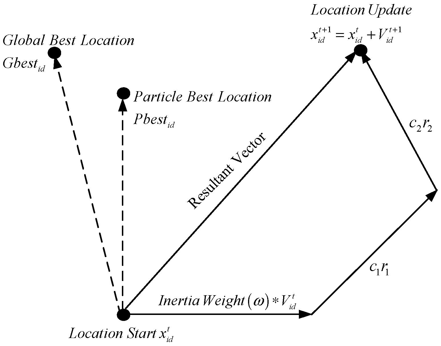
4.1. A Brief Review of PSO Algorithm

PSO is a stochastic algorithm used to obtain the most suitable solution for the optimization problems and was proposed by Kennedy in 1995. The algorithm of PSO is based on the simulation of behavior in which flock of birds flies together in a multi-dimensional search space, adjusting their movements and distances is to discover an optimum objective, subject to the constraints imposed [94]. PSO is described graphically in Figure 1.

Mathematically, PSO velocity and position formulas are expressed by Equations (29) and (30).

$$v_{id}^{t+1}=\stackrel{Inertial\hspace{0.17em}Component}{\overbrace{\omega v_{id}^t}}+\hspace{0.17em}\hspace{0.17em}\hspace{0.17em}\hspace{0.17em}\stackrel{Cognitive\hspace{0.17em}\hspace{0.17em}Component}{\overbrace{c_1{r}_1()(pbes{t}_{id}-x_{id}^t)}}\hspace{0.17em}\hspace{0.17em}\hspace{0.17em}+\hspace{0.17em}\hspace{0.17em}\hspace{0.17em}\stackrel{Social\hspace{0.17em}\hspace{0.17em}Component}{\overbrace{c_2{r}_2()(gbes{t}_{gd}-x_{id}^t)}},$$

(29)

$$x_{id}^t=x_{id}^t+v_{id}^{t+1};\hspace{0.17em}i=1,2,\dots ,n;d=1,2,\dots ,m$$

(30)

where i is particle’s index, t discrete-time index, d dimension being considered, n number of particles in a group, m dimensions of a particle, ω inertia weight factor, and c₁, c₂ acceleration coefficient for the cognitive and social components, respectively [95,96,97].

4.2. Review of PSO Applied to OED Incorporating RESs

In [98], the authors proposed a linearized network model in the form of the DC power flow model while considering the thermal limits of transmission lines and real power constraints. The cost curves for generating units have been developed in the form of a piecewise linear model, and simulation was analyzed on HOMER software for intermittent RESs, specifically wind turbines. They concluded that the steady-state analysis of the power system with the inclusion of RESs is very important and results in significant cost saving.

Reference [99] presented a chaos PSO based algorithm for dispatch cost reduction of hybrid power system by treating wind and solar power generations as negative load. The proposed algorithm gives the best convergence competence and search performance in evaluation. They concluded that chaos PSO provides better results in convergence time and efficient mechanism for the use of RESs.

The incorporation of RESs in the power system reduces the emissions that pollute or environment. However, large-scale power generation using these resources is possible only at locations that are hundreds or thousands of kilometers away from the load centers. This emphasizes the use of a properly designed dispatch mechanism [100].

The authors in [101] designed the double-weighted PSO (DWPSO) to cater to the non-convexity in combined emission economic dispatch (CEED) when intermittent wind energy is used. Equation (31) shows the formula used for conversion double objective CEED problem into a single optimization problem.

$$\min \left\{C={\displaystyle \sum _{i=1}^m{F}_i\left(P_i\right)}+h{\displaystyle \sum _{i=1}^m{E}_i\left(P_i\right)}\right\}$$

(31)

where h is the ratio between maximum fuel cost and maximum emission for each unit given in Equation (32).

$$h=\frac{F_i\left(P_i^{\max }\right)}{E_i\left(P_i^{\max }\right)}$$

(32)

The designed algorithm resulted in the successful reduction of the fuel cost by providing a solution to the non-convex wind penetration in the power system. The authors also concluded that the solution proposed also showed a decline in perilous emissions.

Reference [102] developed a mechanism of optimal operation for the distributed generation at the micro-grid (MG) level, in contrast to the algorithm developed for large-scale generation presented in [101]. The authors also performed the resource estimation for wind and calculated the power that could be extracted from wind and PV (without forecasting). They also focused on the formulations for the economic operation of small-scale energy zones. The designed cost function for generation and operation and maintenance are given in Equations (33) and (34), respectively.

$$Cos{t}_{gen,si}=Cos{t}_{gen,MT,si}+Cos{t}_{gen,FC,si}+Cos{t}_{gen,CHP,si}$$

(33)

$$Cos{t}_{O\&M,s}=Cos{t}_{O\&M,WT,s}+Cos{t}_{O\&M,PV,s}+Cos{t}_{O\&M,MT,s}+Cos{t}_{O\&M,FC,s}+Cos{t}_{O\&M,CHP,s}$$

(34)

where these functions are of generation cost, transaction powers, and O&M cost pollutant emission. The authors solved the dispatch problem in the imperialist competitive algorithm (ICA), and the results proved to be better than the Monte-Carlo simulation (MCS). In all the cases mentioned above, the requirement is to satisfy the load requirements as mentioned in Equation (35).

$$\begin{array}{l}{\displaystyle \sum _i^n{P}_i=P_D+P_l}\\ P_{Gi}^{\min }\le P_{Gi}\le P_{Gi}^{Max},i=1,2,\dots ,N_G\end{array}$$

(35)

where P_t, P_D, and P_l are total power, power demand, and power losses respectively, and the second portion of Equation (35) presents the generation limits that must be met to keep the system balanced.

4.3. Constraints Handling by PSO

Despite many benefits, the application of PSO requires proper consideration of certain constraints such as frequency fluctuation, ramp-rate limits, compensation of load variation, and battery storage. Some prominent schemes to manage these constraints while performing OED of the generated energy are discussed in the following sub-sections.

4.3.1. Compensation for Load and Voltage Variation

The occurrence of load variation is a major limitation, as it disturbs the normal operation of the power system. The load variation is eminent, but the researchers and planners are interested in designing the mechanisms that have the capability of compensating the load variations. A model of Multi-Microgrid (MMG) for voltage regulation against load variations has already been discussed.

Reference [103] proposed an optimal generation rescheduling mechanism designed through dynamic PSO, for RESs to overcome load variations. Dynamic PSO worked by the variation in the acceleration co-efficient, and this resulted in fast convergence, improved global search capability, and achievement of the global optima at the end-stage. The calculation for the amount of solar and wind powers was performed using Equation (36).

$$P_S+P_W\le \eta \times P_D^a$$

(36)

where $P_S$, $P_W$, and $P_D^a$ are the solar power, wind power, and the actual load demand, respectively. Solar and wind powers generated have been taken as a negative load. The effectiveness of the proposed solar-wind system with the hybrid system emerged with a reduction in the fuel cost. The formula for calculation of the percentage reduction is given in Equation (37).

$$\Delta C=\left(1-\frac{F_{fR}}{F_{fN}}\right)\times 100$$

(37)

where $F_{fR}$ and $F_{fN}$ represent the fuel costs with and without RES. The authors concluded that the presented algorithm prevented premature convergence and also maintained the voltage by scheduling the generation as per load variation. But, the specific class of power generation value was ignored by the authors that is being discussed in the preceding discussions.

The authors in [104] presented Chaos PSO based optimization method for standalone MGs to achieve economic dispatch and voltage compensation. The proposed mechanism controlled not just the electricity but the cooling and heating systems as well. The power balance constraints are given in Equation (38).

$${\displaystyle \sum _{m=1}^Q{P}_m(t)=}{P}_{E.L}(t)-P_{E.L,c}(t);P_H(t)=P_{H,L}(t)\hspace{0.17em}\&P_C(t)=P_{C.L}(t)$$

(38)

where $P_{E.L}(t)$, $P_{H,L}(t)$ and $P_{C.L}(t)$ are electricity, thermal and cooling load of the MG, respectively. The simulations performed by the authors proved the designed system to be capable of effectively solving the optimization problem for different situations while keeping the voltage variations in the limit and improving the overall economic and environmental efficiency.

4.3.2. Control of Frequency Fluctuations

The availability of RESs is never constant over a period of time. This uncertainty in the available supply demands proper consideration of the system frequency. This frequency control is very important in the sense that it enables the system to automatically and dynamically adjust generation to meet the load demand that improves load factor and consumption of energy. Frequency control mechanisms also increase the flexibility of the system components, which encourages the integration of a number of MGs to develop MMGs and supply good quality of energy to the load while keeping the frequency and other power system parameters in their specified limits [105]. Many researchers have investigated and presented different mechanisms to provide frequency control in RES based power system while having a proper plan for OED.

In [106], the authors presented a comprehensive review of the mitigating methods adopted to control the fluctuations of a power system containing PV cells. Load variations cause the system frequency to deviate, and the situation becomes even worse when the solar radiation causes the PV output to vary as well, as it was discussed in [107]. The authors also analyzed that the frequency fluctuations in PV based systems were less than the wind-based systems. However, this difference is of lesser significance as the modern grid system has interconnected hybrid solar and wind power systems. They also proposed that in order to compensate for the drooping frequency due to a rise in load, a battery storage system can be implemented. The authors presented simulation models to demonstrate the presented schemes for controlling power fluctuations especially variations in the frequency of PV sources.

Reference [108] presented a mechanism to control the frequency stability and ED of the power system networks. The authors presented asymptotic stability for integral frequency control to accommodate a decentralized power system. The authors then developed a distributed averaging-based integral (DAI) control that is designed to operate by sense and control system of local frequency. The formula for ED of the generated power is given in Equation (39).

$$\begin{array}{l}\hspace{1em}\hspace{1em}\hspace{1em}\hspace{1em}\hspace{1em}\hspace{1em}\hspace{1em}\hspace{1em}\hspace{1em}\hspace{1em}\underset{\theta ,\hspace{0.17em}u}{\min }\hspace{0.17em}{\displaystyle \sum _{j\in N}\frac{1}{2}{a}_j{u}_j^2}\\ \mathrm{subject} \mathrm{to}\\ \hspace{1em}\hspace{1em}\hspace{1em}\hspace{1em}\hspace{1em}\hspace{1em}\hspace{1em}\begin{array}{l}{p}_j+u_j-{\displaystyle \sum _{k\in N}{B}_{jk}\sin \left({\theta }_j-{\theta }_k\right)=0,\hspace{0.17em}\hspace{0.17em}\hspace{0.17em}\hspace{0.17em}\hspace{0.17em}\hspace{0.17em}\hspace{0.17em}\hspace{0.17em}\hspace{0.17em}\hspace{0.17em}\hspace{1em}\hspace{1em}j\in N}\\ \left|{\theta }_j-{\theta }_k\right|\le {\gamma }_{jk}<\frac{\pi }{2},\hspace{1em}\hspace{1em}\hspace{1em}\hspace{1em}\hspace{1em}\hspace{1em}j,k\in \epsilon \end{array}\end{array}$$

(39)

The explicit synchronization frequency is given by Equation (40).

$${\omega }^{\ast }=\frac{{\displaystyle {\sum }_{j\in N}{p}_j+}{u}_j}{{\displaystyle {\sum }_{j\in N}{D}_j}}$$

(40)

The results concluded that the proposed DAI control system provided the closed-loop stability to the system and achieved the desired ED. These conclusions were also validated by the simulations performed. However, the impact of back-up supply on frequency control was not considered.

The authors in [109] presented a droop control method for the frequency stability of RES based power systems. Unlike [108], the proposed system worked by controlling the charging power through the aggregated participation of the system frequency, which was instated as soon as the system frequency deviated from the rated frequency. The mathematical formula required to be satisfied for the power, while the system frequency remained regulated is given in Equation (41).

$$P_{agg,t,h}=P_{c,grant,t,h}+\Delta P;P_{agg,t,h}\ge P_{force,t,h}$$

(41)

The authors concluded through their results that the proposed system performed well in frequency regulation even when the penetration of RES increased. They also proved that the higher the RES penetration in the power system, the more significant the frequency regulation mechanism.

4.3.3. Regulation of Ramp-Rate Limits

The ramp rate (RR) is defined as the rate of change in power at the given time interval. If the change in power is positive, it is known as a ramp-up, and if the power change is negative, then it is known as a ramp-down event. Ramp rate accounts for the difference in power over the specified time interval [110]. The RR occurs due to the intermittent nature of RES as the wind speed or solar irradiation endures variation during different time intervals of a day. This variation in wind speed or solar radiation causes the power supply to change, thus impacting the overall performance of the power system as it may cause other imbalances to appear and disturb the normal operation of the power system. The wind energy is more prone to these RR limits (RRL) violation than the solar radiation, because of more variation of wind speed during different periods of the day. The overall impact of power generation variation should be considered by the planners to maintain the continuity and reliability of the supply. Many researchers have developed mechanisms to measure and sort-out the RRL violations.

Reference [111] developed an optimal operation mechanism for grid-connected hybrid RESs for residential applications. The designed system incorporated a variety of sources like PV, wind, fuel cell and solar thermal and supplied electricity and heating. The modified PSO performed the optimization problem. The ramp rate occurrence and the fuel cell (FC) assembly, start and stop cycles are given in Equation (42).

$$\begin{array}{l}{P}_{\min }\le P_{FC,i}\le P_{Max}\\ \left(T_{t-1}^{off}-MDT\right)\left(U_i-U_{i-1}\right)\ge 0\\ \left(T_{t-1}^{on}-MUT\right)\left(U_{i-1}-U_i\right)\ge 0\\ P_{FC,i-1}-P_{FC,i}\le \Delta P_d\\ P_{FC,i}-P_{FC,i-1}\le \Delta P_u\end{array}$$

(42)

where $T^{off}$ and $T^{off}$ denote the FC off and on time respectively, and U denotes the on-off status of the FC following the binary system MUT and MDT represents the upper and lower ramp rate limits respectively. The simulation results obtained were after implementation of the proposed system for four different cases, and assessment of the results validated that the proposed hybrid energy system was more cost-effective and simpler than the stand-alone single-source systems, even when the system must supply energy to full load demand. A comparison between the optimization of modified PSO and genetic algorithm (GA) also concluded that modified PSO was more accurate with better convergence time.

In [112], designed a stochastic ED model for hybrid power systems with the wind, solar, and thermal power plants, to solve dynamic economic emission dispatch (DEED) problems while considering the environmental constraints. They used a weighted aggregation method for enabling PSO to solve multi-objective (MO) problems. The RR constraint incorporated in [112] is given in Equation (43).

$$P_{ij}-P_{ij-1}\le U{R}_i;P_{ij-1}-P_{ij}\le D{R}_i$$

(43)

where $U{R}_i$ and $D{R}_i$ are ramp-up and ramp-down for the ith unit, respectively. The authors based on their simulation and results, concluded that the presented model provided an optimal solution to the DEED problem. The developed system tackled the uncertainty and system imbalance issues efficiently and operated the system securely and optimally.

The authors in [113] presented a model for combined economic emission dispatch (CEED) with a PV system integrated with serval thermal generating plants. The formulated problem was tackled through a decomposition framework that divided the problem into two sub-problems. PSO, Newton-Raphson method, and binary integer programming techniques were incorporated in the designed mechanism. The proposed solution for the optimization problem is given in Equation (44).

$$\underset{P_i,U{s}_j,P{s}_k}{\min }{\displaystyle \sum _{i=1}^n\left(F_i\left(P_i\right)+E_i\left(P_i\right)\right)}+{\displaystyle \sum _{j=1}^m{G}_j-U{s}_j}-{\displaystyle \sum _k^{NB}P{s}_k}-{\displaystyle \sum _{j=1}^{m}U{s}_j}$$

(44)

The authors concluded that the presented mechanism could reduce overall fuel costs and had the potential to reduce emissions by enhancing the share of solar generation in the power system. The hybrid optimization scheme also provided an optimal solution for the ED of generation while satisfying RRL.

4.3.4. Storage Mechanism as a Solution

RESs based supply keeps on varying throughout the time period besides, their supply is also not available during a day as wind flow can vary, or a cloud cover may emerge at any time [114,115,116]. This intermittent nature of these sources also gives rise to certain issues such as frequency fluctuations and RRL that requires proper backup arrangement to keep up with the continuous load demand. The backup system can be of two categories:

(i)

Thermal Power Generation is dependable, but it presents major issues such as a rise in carbon emissions, an increase in fuel cost, and special consideration is required in system coordination. We cannot use thermal plants as backup generation only as they take a significant amount of time in their start-up, and fuel cost for spinning reserve contributes to disturbing the economic dispatch that is a major concern in current power system.

(ii)

Battery Storage compensation through batteries is a modern age replacement of backup thermal plants. It requires a properly designed storage system to provide adequate power to supply the load when power from RESs is lesser than the demand. The battery storage system also provides an additional benefit of peak shaving as RES starts supplying an excessive supply for storage [117,118]. The major concern is of designing a properly designed storage system to achieve the optimum cost-saving and stability of the power system.

Many researchers have presented mechanisms based on backup storage systems that maintain continuous supply according to the load demand while keeping the system constraints within their limits.

In [119], the authors discussed the economic allocation of energy storage systems for Wind Power Distribution. The authors argued that the improper size selection and wrong placement of the storage units cause voltage instability and an undesired increase in the cost of the power system. To solve this, issue the authors presented an algorithm based on the hybrid multi-objective PSO (HMOPSO) to improve the voltage profile and cost of the power system. The proposed algorithm was designed by the combination of MOPSO, non-dominant sorting GA, and probabilistic load flow techniques. The mathematical relation used for computation of the operational cost is given in Equation (45).

$$Cos{t}_i={\displaystyle \sum _{j=1}^{NG}C(P_{G_i})+C_w+C_s}$$

(45)

where $C(P_{G_i})$, $C_w$ and $C_s$ are the fuel cost of the generator, cost of wind power generator, and cost of energy storage system, respectively. They concluded through the presented simulation results that the system provided proper placement and sizing of the Energy Storage System (ESS) as well as minimizing the total operational cost and improved the voltage profile. But, the power compensation extracted from batteries was slow.

The authors in [120] presented optimization of the battery ESS (BESS) through PSO implemented on stand-alone MGs. The proposed method was designed to install a battery of optimum size to compensate for the load demand when required and simultaneously control the frequency to avoid any instability occurrence in the power system. The proposed model was also compared on an economic basis with some of the available modern technologies. The authors also discussed some of the materials used in batteries to find out the optimum material for better battery storage. They proposed polysulfide-bromine based BESS to be cost-effective than the redox-based BESS for long-duration applications. The formulas used by the authors for BESS calculation are given in Equation (46).

$$E_{bac}=\frac{r_{bp}}{1+S{T}_{bp}}{I}_{BESS};\hspace{1em}\hspace{1em}{I}_{BESS}=\frac{E_{bt}-E_{bac}-E_{b1}}{r_{bt}+r_{bs}};\hspace{1em}\hspace{1em}{E}_{b1}=\frac{r_{b1}}{1+S{T}_{b1}}{I}_{BESS}$$

(46)

where $I_{BESS},E_{b1},E_{bt},E_{bac},r_{bp}$ and $r_{b1}$ are current through the battery, battery resistance, V_phase of the battery side, V_open-circuit of battery, self-discharge resistance, and over-voltage resistance, respectively. Based on the presented results, the authors concluded that the presented system offered very fast compensation for active power that improved the dynamic stability of the power system. The results also validated the significance of the BESS based PSO mechanism for optimum sizing of the storage system.

Reference [121] emphasized the use of ESS to tackle the inherent uncertainty of the wind power system to make the power system more reliable. The authors discussed several technologies available for ESS of different stability purposes and concluded that the properly designed battery system is key to success. The formulas incorporated for ESS power output and remaining energy level (REL) is given in Equation (47).

$$P_{bess}^{ord}=\frac{-s{T}_f}{1+s{T}_f}{P}_{wind};REL=\frac{P_{bess}^{ord}}{s}=\frac{T_f}{1+s{T}_f}{P}_{wind}$$

(47)

where $T_f$ is time constant. It is also clear from Equations (46) and (47) that the larger the value of time-constant, higher will be smoothing effect and larger will be ESS power.

The authors concluded that recent models focused on the daily dispatch of the ESS operation and control to compensate for the power fluctuations [122]. The authors also discussed the technical constraints, some of which have already been discussed in this paper for the OED of RESs. The authors also emphasized the significance of time-constant in the smoothing effect along-with system power stability and capacity rating.

The authors in [123] designed a mechanism of optimal energy storage system (ESS) along-with a PV generation system. The mechanism presented by the authors was based on four steps, i.e., prediction of load and daily power generation, an optimization process for best battery power “P^b” and state of battery charge “SOC^b”, power requests calculus, and E-broker auction algorithms. The value of P^b was computed using Equation (48).

$$P^b=2\cdot P_{cont}\cdot x_p$$

(48)

where $x_p$ is the optimization variable. SOC^b was used to trigger the power requests from the system. The method avoided the scenario faced by researchers where they had to impose a division on the battery peak shaving and energy shifting as it optimized suitable variables and prevented the ESS from capacity wasting. The presented model also prevented power losses and unforeseen peaks occurring due to the supply or absorption of power by optimizing the boundaries of battery behavior. However, the system was not effective for active distribution systems (ADSs).

Reference [124] presented a fuzzy multi-objective bi-level problem for the planning of ESS in (ADS). The authors designed a model using PSO and differential evaluation (DE) for the solution to the mentioned problem. They considered two scenarios of ADSs like peak load shaving and failure status responsibility support system. The mechanism worked by dividing the yearly data into 365 intervals according to the load demand and power output by the REGs. The objective functions developed for peak load shaving, restraining voltage ESS reserve capability are given in Equations (49) and (50), respectively.

$$\begin{array}{l}\min f_1=\min {{\displaystyle \sum _{t=1}^{24}\left(P_{NL}\left(t\right)\hspace{0.17em}-\hspace{0.17em}{P}_{NL,average}\right)}}^2\\ \min f_2=\min {{\displaystyle \sum _{t=2}^{24}\left(P_{NL}\left(t\right)\hspace{0.17em}-\hspace{0.17em}{P}_{NL}\left(t-1\right)\right)}}^2\\ \min f_3=\min \left(\frac{1}{{\displaystyle \sum _{t=1}^{24}{P}_{ava}\left(t\right)}}\right)\end{array}$$

(49)

and

$$P_{ava}\left(t\right)=\min \left\{P_{ESS}^R,\frac{\left(ESS\left(t-1\right)-E_{ESS}^{\min }\right){\eta }_D}{\Delta t}\right\}$$

(50)

where $P_{NL,average}$ is the average of the net load demand of the ADS, $ESS(t)$ is energy stored in battery bank at time t, and $E_{ESS}^{\min }$ is the minimum energy stored in the battery bank of the ESS.

Based on the simulation results, the authors concluded that the propped scheduling model contributes to obtaining a reasonable planning scheme by taking into consideration the ESS operation strategy. The system implemented in designing a proper ESS can help in tackling the time-varying nature of RESs and the load demand as well.

The authors in [125] presented a stochastic planning and scheduling model for ESSs to handle the congestion in the electric power systems consisting of RESs. The model provided a design mechanism for charging the dis-charging of ESSs to handle the intermittent nature of RESs. The output power of wind and solar using Gaussian probability density function (PDF) and Monte-Carlos simulation (MCS) along-with ESS to tackle unpredictability. The objective functions for congestion management and ESS cost minimization are mentioned in Equations (51), (52) and (53), respectively.

$$o{f}_{cm}=C_n\hspace{0.17em}+\hspace{0.17em}I{N}_{ESS}$$

(51)

$$I{N}_{ESS}=\left(D{V}_E\times P_{ESS}\times I{P}_E\right)\times EAC$$

(52)

$$C_n=\{{\displaystyle \sum _{ll=1}^{mll}\left({\displaystyle \sum _{nl=1}^{NL}\left(S_{nl}^{ll}\times FT{R}_{nl}^{ll}\right)}\right)}\}\times {\mathrm{T}}_{an}$$

(53)

where $I{N}_{ESS}$ is annual installation cost of ESS, $EAC$ is applied converter for life-cycle, $C_n$ is power flow through all lines, and $FTR$ is financial transmission right for daily congestion cost, respectively. The planning system requires three identical ESSs to manage the congestion and cost of the system. The network without ESS cannot meet the constraints, and simulation results concluded that ESS not only reduced the loss but also improved the voltage profile and stability margin.

Table 6. Constraints and their solutions for optimal economic (OED) of Renewable Energy Sources (RESs).

Constraints	Presented Model	Objective Function	Reference
Load and Voltage Variations	$\begin{array}{l}{P}_D^a+P_L-{\displaystyle \sum _{i=1}^{N_G}{P}_{Gi}}=0\\ P_D^a=P_D^t-\left(P_s+P_W\right)\end{array}$	$\begin{array}{l}\min F_f\left(P_{Gi}\right)\\ ={\displaystyle \sum _{i=1}^{N_G}\left(a_i+b_i{P}_{Gi}+c_i{P}_{Gi}^2\right)}\end{array}$	$\mathrm{Here} P_D^a$$, P_L$$, P_s$$\mathrm{and} P_W$ are the load demand, transmission losses, solar and wind powers, respectively [103,104].
Frequency Fluctuations	$\begin{array}{l}{P}_{force,t,h}={\displaystyle \sum _{k=1}^{K_{t,h}}{P}_{rate,k}^{U_n}+{\displaystyle \sum _{j=1}^{M_{t,h}}{P}_{rate,j}^M}}\\ P_{c,\max ,t,h}={\displaystyle \sum _{i=1}^{N_{t,h}}{P}_{rate,i}}\end{array}$	$\min {\displaystyle \sum _{t=1}^T\left\{{\displaystyle \sum _{g=1}^{N_g}\left(\begin{array}{l}{a}_g\cdot {\left(P_{g,t}^{G,ref}\right)}^2+\\ b_g\cdot P_{g,t}^{G,ref}+c_g\end{array}\right)}\right\}}$	[105,106,107,108,109]
Ramp-Rate Limits	$\begin{array}{l}{F}_i\left(P_i\right)={\alpha }_i{P}_i^2+{\beta }_i{P}_i+{\gamma }_i+\\ {\epsilon }_i\exp \left({\delta }_i\times P_i\right)\end{array}$	$\begin{array}{l}\underset{P_i,U{s}_j,P{s}_k}{\min }{\displaystyle \sum _{i=1}^n\left(F_i\left(P_i\right)+E_i\left(P_i\right)\right)}+\\ {\displaystyle \sum _{j=1}^m{G}_j-U{s}_j}-{\displaystyle \sum _k^{NB}P{s}_k}-{\displaystyle \sum _{j=1}^{m}U{s}_j}\end{array}$	[110,111,112,113]
Storage Mechanism	$\begin{array}{l}{P}_i-V_i{\displaystyle \sum _{j=1}^N{V}_j\left(G_{ij}\cos {\delta }_{ij}+B_{ij}\sin {\delta }_{ij}\right)}=0\\ Q_i-V_i{\displaystyle \sum _{j=1}^N{V}_j\left(G_{ij}\sin {\delta }_{ij}-B_{ij}\cos {\delta }_{ij}\right)}=0\end{array}\}$	$\begin{array}{l}\min f_1={\displaystyle \sum _{i=1}^5\mathrm{Pr}o{b}_i\cdot Cos{t}_i}\\ \min f_2={\displaystyle \sum _{k=1}^n{\left(\frac{V_k-V_k^{spec}}{\Delta V_k^{\max }}\right)}^2}\end{array}\}$	[114,115,116,117,118,119,120,121,122,123,124,125]

summarizes the discussed solutions to the constraints along-with their presented models and objective functions.

5. Conclusions

This paper reviews the constraints faced and their solutions for reliable, efficient, cost-effective, and sustainable RESs based power systems. The fluctuating RES input power categorized in time and space has different solutions. In the time domain, forecasting helps plan for the supply-demand mismatch. In the spatial domain, different regions across vast space have different generation capabilities and hence can be used to balance out load mismatch. The combination of time and space variations, both of which have different solutions integrated gives the best overall system solution. The intermittency of RESs poses a major hurdle in their large-scales implementations but, supply forecasting (i.e., wind speed and solar irradiance) helps power system planners to design and implement large RESs based on power generation farms. WD emerges as an accurate, reliable and fast technique for predicting resource availability during a specified time period. The forecasting mechanisms may also require the incorporation of NN for the correction of an error in the predicted value to make the system even more precise. The RESs dependent power systems also have to face some other constraints such as load and voltage variation, frequency fluctuations, ramp-rate limits, and energy storage mechanisms in OED. The proposed mechanisms and algorithms for the solution of these constraints have been discussed and summarized. The review showed that the consideration of these constraints improves the performance of the power system for optimal economic dispatching. This paper comprehensively provides a manuscript for investors and power system planners to be able to learn about constraints and their available solutions, and it can be beneficial for researchers by providing a broad source for their literature review.

References

1. Hansen, J.; Kharecha, P.; Sato, M.; Masson-Delmotte, M.; Ackerman, F.; Beerling, J.D.; Hearty, P.J.; Hoegh-Guldberg, O.; Hsu, S.L.; Parmesan, C.; et al. Assessing dangerous climate change, required reduction of carbon emissions to protect young people, future generations and nature. PLoS ONE 2013, 8, e81648. [Google Scholar] [CrossRef] [PubMed]
2. Nuclear Power: Totally Unqualified to Combat Climate Change. Available online: https://worldbusiness.org/ (accessed on 21 December 2018).
3. Ela, E.; O’Malley, M. Studying the variability and uncertainty impacts of variable generation at multiple timescales. IEEE Trans. Power Syst. 2012, 27, 1324–1333. [Google Scholar] [CrossRef]
4. Widén, J.; Carpman, N.; Castellucci, V.; Lingfors, D.; Olauson, J.; Remouit, F.; Bergkvist, M.; Grabbe, M.; Waters, R. Variability assessment and forecasting of renewables: A review for solar, wind, wave and tidal resources. Renew. Sustain. Energy Rev. 2015, 44, 356–375. [Google Scholar] [CrossRef]
5. Milligan, M.; Kirby, B. Calculating Wind Integration Costs: Separating Wind Energy Value from Integration Cost Impacts; No. NREL/TP-550-46275; National Renewable Energy Lab.(NREL): Golden, CO, USA, 2009.
6. Rondina, J.M. Technology Alternative for Enabling Distributed Generation. IEEE Lat. Am. Trans. 2016, 14, 4089–4096. [Google Scholar] [CrossRef]
7. Distributed Generation. Environmental & Energy Study Institute. Available online: https://www.eesi.org/topics/distributed-generation/description (accessed on 27 December 2018).
8. Libra, M.; Beránek, V.; Sedláček, J.; Poulek, V.; Tyukhov, I.I. Roof photovoltaic power plant operation during the solar eclipse. Sol. Energy 2016, 140, 109–112. [Google Scholar] [CrossRef]
9. Distributed Generation. OFGEM. Available online: https://www.ofgem.gov.uk/electricity/distribution-networks/connections-and-competition/distributed-generation (accessed on 27 December 2018).
10. Microgrids. Grid Integration group, Energy Storage and Distributed Sources Division. Available online: https://building-microgrid.lbl.gov/microgrid-definitions (accessed on 29 December 2018).
11. Khan, I.; Zhang, Y.; Xue, H.; Nasir, M. A Distributed Coordination Framework for Smart Microgrids. In Smart Microgrids; Springer: Cham, Switzerland, 2019; pp. 119–136. [Google Scholar]
12. Wan, Q.; Zhang, W.; Xu, Y.; Khan, I. Distributed control for energy management in a microgrid. In Proceedings of the IEEE/PES Transmission and Distribution Conference and Exposition (T&D), Dallas, TX, USA, 3–5 May 2016; pp. 1–5. [Google Scholar]
13. Zhaoyun, Z.; Wenjun, Z.; Mei, Y.; Li, K.; Zhi, Z.; Yang, Z.; Guozhong, L.; Na, Y. Application of Micro-Grid Control System in Smart Park. J. Eng. 2019, 2019, 3116–3119. [Google Scholar] [CrossRef]
14. Weibull Analysis, An Overview of Basic Concepts. Available online: https://www.weibull.com/ (accessed on 22 December 2018).
15. More, A.; Deo, M.C. Forecasting wind with neural networks. Mar. Struct. 2003, 16, 35–49. [Google Scholar] [CrossRef]
16. Kirschen, D.S.; Ma, J.; Silva, V.; Belhomme, R. Optimizing the flexibility of a portfolio of generating plants to deal with wind generation. In Proceedings of the IEEE Power and Energy Society General Meeting, Detroit, MI, USA, 24–28 July 2011; pp. 1–7. [Google Scholar]
17. Gerven, M.V.; Bohte, S. Artificial neural networks as models of neural information processing. Front. Comput. Neurosci. 2018, 11, 114. [Google Scholar] [CrossRef]
18. Stergiou, C.; Siganos, D. Neural Networks. Available online: http://www.imperial.ac.uk/computing (accessed on 22 December 2018).
19. Nasle, A.; Nasle, A. Systems and Methods for Real-Time Forecasting and Predicting of Electrical Peaks and Managing the Energy, Health, Reliability, and Performance of Electrical Power Systems Based on an Artificial Adaptive Neural Network. U.S. Patent 9,846,839, 19 December 2017. [Google Scholar]
20. Jordehi, A.R. How to deal with uncertainties in electric power systems? A review. Renew. Sustain. Energy Rev. 2018, 96, 145–155. [Google Scholar] [CrossRef]
21. Ba˜nos, R.; Agugliarob, F.M.; Montoyab, F.G.; Gila, C.; Alcaydeb, A.; Gómezc, J. Optimization methods applied to renewable and sustainable energy: A review. Renew. Sustain. Energy Rev. 2011, 15, 1753–1766. [Google Scholar] [CrossRef]
22. Gamarra, C.; Guerrero, J.M. Computational optimization techniques applied to micro-grids planning: A review. Renew. Sustain. Energy Rev. 2015, 48, 413–424. [Google Scholar] [CrossRef]
23. Alizadeh, M.I.; Moghaddam, M.P.; Amjady, N.; Siano, P.; Eslami, M.K.S. Flexibility in future power systems with high renewable penetration: A review. Renew. Sustain. Energy Rev. 2016, 57, 1186–1193. [Google Scholar] [CrossRef]
24. García, F.; Bordons, C. Optimal economic dispatch for renewable energy microgrids with hybrid storage using Model Predictive Control. In Proceedings of the IECON 2013—39th Annual Conference of the IEEE Industrial Electronics Society, Vienna, Austria, 10–13 November 2013; pp. 7932–7937. [Google Scholar]
25. Bai, Q. Analysis of Particle Swarm Optimization Algorithm. Comput. Inf. Sci. 2010, 3, 180. [Google Scholar] [CrossRef]
26. Settles, M. An introduction to particle swarm optimization; University of Idaho: Moscow, Russia, 2005. [Google Scholar]
27. Rini, D.P.; Shamsuddin, S.M.; Yuhaniz, S.S. Particle swarm optimization: Technique, system and challenges. Int. J. Comput. Appl. 2011, 14, 19–26. [Google Scholar] [CrossRef]
28. Abbas, G.; Gu, J.; Farooq, U.; Asad, M.U.; El-Hawary, M. Solution of an Economic Dispatch Problem Through Particle Swarm Optimization: A Detailed Survey—Part I. IEEE Access 2017, 5, 15105–15141. [Google Scholar] [CrossRef]
29. Abbas, G.; Gu, J.; Farooq, U.; Raza, A.; Asad, M.U.; El-Hawary, M. Solution of an Economic Dispatch Problem Through Particle Swarm Optimization: A Detailed Survey—Part II. IEEE Access 2017, 5, 24426–24445. [Google Scholar] [CrossRef]
30. Jordehi, A.R. Particle swarm optimisation (PSO) for allocation of FACTS devices in electric transmission systems: A review. Renew. Sustain. Energy Rev. 2015, 52, 1260–1267. [Google Scholar] [CrossRef]
31. Sinha, S.; Chandel, S.S. Review of recent trends in optimization techniques for solar photovoltaic–wind based hybrid energy systems. Renew. Sustain. Energy Rev. 2015, 50, 755–769. [Google Scholar] [CrossRef]
32. Kirby, B.; Hirst, E. Customer-Specific Metrics for the Regulation and Load-Following Ancillary Services; ORNL/CON-474; Oak Ridge National Laboratory: Oak Ridge, TN, USA, 2000.
33. Kariyawasam, K.; Karunarathna, K.; Karunarathne, R.; Kularathne, M.; Hemapala, K. Design and Development of a Wind Turbine Simulator Using a Separately Excited DC Motor. Smart Grid Renew. Energy 2013, 4, 259–265. [Google Scholar] [CrossRef]
34. Genc, A.; Erisoglu, M.; Pekgor, A.; Oturanc, G.; Hepbasli, A.; Ulgen, K. Estimation of Wind Power Potential Using Weibull Distribution. Energy Sources 2005, 27, 809–822. [Google Scholar] [CrossRef]
35. Zhang, J.; Hodge, B.-M.; Miettinen, J.; Holttinen, H.; Lázaro, E.G.; Cutululis, N.; L-Palima, M.; Sorensen, P.; Lovholm, A.L.; Berge, E.; et al. Analysis of Variability and Uncertainty in Wind Power Forecasting: An International Comparison. In Proceedings of the 12th International Workshop on Large-Scale Integration of Wind Power into Power Systems, London, UK, 22–24 October 2013. [Google Scholar]
36. Reza, S.E.; Zaman, P.; Ahammad, A.; Ifty, I.Z.; Nayan, M.F. A study on data accuracy by comparing between the Weibull and Rayleigh distribution function to forecast the wind energy potential for several locations of Bangladesh. In Proceedings of the 4th International Conference on the Development in the in Renewable Energy Technology (ICDRET), IEEE, Dhaka, Bangladesh, 7–9 January 2016; pp. 1–5. [Google Scholar]
37. Stoutenburg, E.D.; Jenkins, N.; Jacobson, M.Z. Variability and uncertainty of wind power in the California electric power system. Wind Energy 2014, 17, 1411–1424. [Google Scholar] [CrossRef]
38. Zhang, J.; Wang, J.; Wang, X. Review on probabilistic forecasting of wind power generation. Renew. Sustain. Energy Rev. 2014, 32, 255–270. [Google Scholar] [CrossRef]
39. Reliability Basics: Reliability Engineering Resources. The eMagzine for Reliability Professional. Issue 7. 2001. Available online: https://www.weibull.com/ (accessed on 22 December 2018).
40. Ela, E.; Kirby, B. ERCOT Event on February 26, 2008, Lessons Learned; National Renewable Energy Laboratory: Golden, CO, USA, 2008.
41. Papoulis, A.; Papoulis, S. Probability, Random Variables and Stochastic Processes, 4th ed.; McGraw-Hill: Boston, MA, USA, 2002; ISBN 0-07-366011-6. [Google Scholar]
42. Jiang, R.; Murthy, D.N.P. A study of Weibull shape parameter: Properties and significance. Reliab. Eng. Syst. Saf. 2011, 96, 1619–1626. [Google Scholar] [CrossRef]
43. Amari, S.; Nagaoka, H. Methods of Information Geometry; American Mathematical Society and Oxford University Press: Providence, RI, USA, 2000; p. 206. ISBN 0-8218-0531-2. [Google Scholar]
44. Galambos, J.; Simonelli, I. Products of Random Variables: Applications to Problems of Physics and to Arithmetical Functions; Marcel Dekker, Inc.: New York, NY, USA, 2004; Volume 1, pp. 139–140. ISBN 0-8247-5402-6. [Google Scholar]
45. Clarkson, E. Comparison of Weibull and Normal Distributions; NCAMP Documents/Publications, NCAMP (NASA), Technical Presentations; NASA: Washington, DC, USA, 2013.
46. Merovci, F.; Elbatal, I. Weibull Rayleigh Distribution: Theory and Applications. Appl. Math. Inf. Sci. 2015, 9, 2127–2137. [Google Scholar]
47. Pishgar-Komleh, S.H.; Keyhani, A.; Sefeedpari, P. Wind speed and power density analysis based on Weibull and Rayleigh distributions (A case study: Firouzkooh county of Iran). Renew. Sustain. Energy Rev. 2015, 42, 313–322. [Google Scholar] [CrossRef]
48. Ahmad, M.A.; Raqab, M.Z.; Kundu, D. Discriminating between the Generalized Rayleigh and Weibull Distributions: Some Comparative Studies. Commun. Stat. Simul. Comput. 2017, 46, 4880–4895. [Google Scholar] [CrossRef]
49. Fu, T.; Wang, C. A hybrid wind speed forecasting method and wind energy resource analysis based on a swarm intelligence optimization algorithm and an artificial intelligence model. Sustainability 2018, 10, 3913. [Google Scholar] [CrossRef]
50. Saxena, B.K.; Rao, K.V.S. Comparison of Weibull parameters computation methods and analytical estimation of wind turbine capacity factor using polynomial power curve model: Case study of a wind farm. Renew. Wind Water Sol. 2015, 2, 3. [Google Scholar] [CrossRef]
51. Carrillo, C.; Cidrás, J.; Díaz-Dorado, E.; Montaño, A.F.O. An Approach to Determine the Weibull Parameters for Wind Energy Analysis: The Case of Galicia (Spain). Energies 2014, 7, 2676–2700. [Google Scholar] [CrossRef]
52. Anuradha, M.; Keshavan, B.K.; Ramu, T.S.; Sankar, V. Probabilistic modeling and forecasting of wind power. Int. J. Perform. Eng. 2016, 12, 353–368. [Google Scholar]
53. Nikmehr, N.; Ravadanegh, S.N. Optimal Power Dispatch of Multi-Microgrids at Future Smart Distribution Grids. IEEE Trans. Smart Grid 2015, 6, 1648–1657. [Google Scholar] [CrossRef]
54. Reddy, S.S.; Bijwe, P.R.; Abhyankar, A.R. Joint Energy and Spinning Reserve Market Clearing Incorporating Wind Power and Load Forecast Uncertainties. IEEE Syst. J. 2015, 9, 152–164. [Google Scholar] [CrossRef]
55. Azada, A.K.; Rasul, M.G.; Alam, M.M.; Uddin, S.M.A.; Mondal, S.K. Analysis of wind energy conversion system using Weibull distribution. Procedia Eng. 2014, 90, 725–732. [Google Scholar] [CrossRef]
56. Kim, C.; Gui, Y.; Chung, C.C.; Kang, Y. Model predictive control in dynamic economic dispatch using Weibull distribution. In Proceedings of the IEEE Power & Energy Society General Meeting, Vancouver, BC, Canada, 21–25 July 2013; pp. 1–5. [Google Scholar]
57. Celik, A.K. A statistical analysis of wind power density based on the Weibull and Rayleigh models at the southern region of Turkey. Renew. Energy 2004, 29, 593–604. [Google Scholar] [CrossRef]
58. Sağbaş, A.; Karamanlıoğlu, T. The Application of Artificial Neural Networks in the Estimation of Wind Speed: A Case Study. In Proceedings of the 6th International Advanced Technologies Symposium (IATS’11), Elazığ, Turkey, 18 May 2011; 2011; pp. 16–18. [Google Scholar]
59. Ata, R. Artificial neural networks applications in wind energy systems: A review. Renew. Sustain. Energy Rev. 2015, 49, 534–562. [Google Scholar] [CrossRef]
60. Kadhem, A.A.; Wahab, N.I.A.; Aris, I.; Jasni, J.; Abdalla, A.N. Advanced Wind Speed Prediction Model Based on a Combination of Weibull Distribution and an Artificial Neural Network. Energies 2017, 10, 1744. [Google Scholar] [CrossRef] [Green Version]
61. Quan, H.; Srinivasan, D.; Khosravi, A. Short-Term Load and Wind Power Forecasting Using Neural Network-Based Prediction Intervals. IEEE Trans. Neural Netw. Learn. Syst. 2014, 25, 303–315. [Google Scholar] [CrossRef]
62. Quan, H.; Srinivasan, D.; Khosravi, A.; Nahavandi, S.; Creighton, D. Construction of Neural Network-Based Prediction Intervals for Short-Term Electrical Load Forecasting. In 2013 IEEE Computational Intelligence Applications in Smart Grid (CIASG); IEEE: Piscataway, NJ, USA, 2013; pp. 66–72. [Google Scholar]
63. Peng, H.; Liu, F.; Yang, X. A hybrid strategy of short term wind power prediction. Renew. Energy 2012, 50, 590–595. [Google Scholar] [CrossRef]
64. Mohammadi, K.; Shamshirband, S.; Yee, P.L.; Petkovi, D.; Zamani, M.; Chaudary, S. Predicting the wind power density based upon extreme learning machine. Energy 2015, 86, 232–239. [Google Scholar] [CrossRef]
65. Shamshirband, S.; Mohammadi, K.; Tong, C.W.; Petković, D.; Porcu, E.; Mostafaeipour, A.; Chaudary, S.; Sedaghat, A. Application of extreme learning machine for estimation of wind speed distribution. Clim. Dyn. 2016, 46, 1893–1907. [Google Scholar] [CrossRef]
66. Xu, Y.; Shi, L.; Ni, Y. Deep-learning-based scenario generation strategy considering correlation between multiple wind farms. J. Eng. 2017, 13, 2207–2210. [Google Scholar] [CrossRef]
67. Huang, C.J.; Kuo, P.H. A short-term wind speed forecasting model by using artificial neural networks with stochastic optimization for renewable energy systems. Energies 2018, 11, 2777. [Google Scholar] [CrossRef] [Green Version]
68. Zhang, Y.; Zhang, C.; Zhao, Y.; Gao, S. Wind speed prediction with RBF neural network based on PCA and ICA. J. Electr. Eng. 2018, 69, 148–155. [Google Scholar] [CrossRef] [Green Version]
69. Khan, G.M.; Ali, J.; Mahmud, S.A. Wind power forecasting—An application of machine learning in renewable energy. In Proceedings of the International Joint Conference on Neural Networks (IJCNN), Beijing, China, 6–11 July 2014; pp. 1130–1137. [Google Scholar]
70. World Energy Sources, Solar-2016. World Energy Council. Available online: https://www.worldenergy.org/wp-content/uploads/2017/03/WEResources_Solar_2016.pdf (accessed on 1 October 2019).
71. Shi, G. A Data Driven Approach to Solar Generation Forecasting. 2017. Thesis. ALL. 156. Available online: https://surface.syr.edu/thesis/156/ (accessed on 1 October 2019).
72. Bushong, S. Advantages and Disadvantages of a Solar Tracker System; Solar Power World: Cleveland, OH, USA, 2016. [Google Scholar]
73. Beránek, V.; Olšan, T.; Libra, M.; Poulek, V.; Sedláček, J.; Dang, M.Q.; Tyukhov, I. New monitoring system for photovoltaic power plants’ management. Energies 2018, 11, 2495. [Google Scholar] [CrossRef] [Green Version]
74. Zhang, J.; Florita, A.; Hodge, B.; Lu, S.; Hamann, H.F.; Banunarayanan, V.; Brockway, A.M. A suite of metrics for assessing the performance of solar power forecasting. Sol. Energy 2015, 111, 157–175. [Google Scholar] [CrossRef] [Green Version]
75. Geoffrey, H. Reflections--The Economics of Renewable Energy in the United States. Rev. Environ. Econ. Policy 2009, 4, 139–154. [Google Scholar]
76. Kumara, S.; Sarkara, B. Design for reliability with weibull analysis for photovoltaic modules. Int. J. Curr. Eng. Technol. 2013, 3, 129–134. [Google Scholar]
77. Langella, R.; Proto, D.; Testa, A. Solar Radiation Forecasting, Accounting for Daily Variability. Energies 2016, 9, 200. [Google Scholar] [CrossRef] [Green Version]
78. Peruchena, C.M.F.; Ramı´rez, L.; Silva-Pe´rez, M.A.; Lara, V.; Bermejo, D.; Gasto´n, M.; Moreno-Tejera, S.; Pulgar, J.; Liria, J.; Macı´as, S.; et al. A statistical characterization of the long-term solar resource: Towards risk assessment for solar power projects. Sol. Energy 2016, 123, 29–39. [Google Scholar] [CrossRef]
79. Basri, M.J.M.; Abdullah, S.; Azrulhisham, E.A.; Harun, K. Higher order statistical moment application for solar PV potential analysis. In Proceedings of the AIP Conference Proceedings AIP Publishing, Penang, Malaysia, 10–12 April 2016; Volume 1782, p. 050004. [Google Scholar]
80. Munkhammar, J.; Widén, J.; Rydén, J. On a probability distribution model combining household power consumption, electric vehicle home-charging and photovoltaic power production. Appl. Energy 2015, 142, 135–143. [Google Scholar] [CrossRef]
81. Ayodele, T.R. Determination of Probability Distribution Function for Global Solar Radiation: Case Study of Ibadan, Nigeria. Int. J. Appl. Sci. Eng. 2015, 13, 233–245. [Google Scholar]
82. Maraj, A.; Londo, A.C.; Firat, C.; Karapici, R. Solar Radiation Models for the City of Tirana, Albania. Int. J. Renew. Energy Res. 2014, 4, 413–420. [Google Scholar]
83. Arias-Rosales, A.; Mejía-Gutiérrez, R. Optimization of V-Trough photovoltaic concentrators through genetic algorithms with heuristics based on Weibull distributions. Appl. Energy 2018, 212, 122–140. [Google Scholar] [CrossRef]
84. Yadav, A.K.; Chandel, S.S. Solar radiation prediction using Artificial Neural Network techniques: A review. Renew. Sustain. Energy Rev. 2014, 33, 772–781. [Google Scholar] [CrossRef]
85. Behravesh, V.; Keypour, R.; Foroud, A.A. Stochastic analysis of solar and wind hybrid rooftop generation systems and their impact on voltage behavior in low voltage distribution systems. Sol. Energy 2018, 166, 317–333. [Google Scholar] [CrossRef]
86. Chiteka, K.; Enweremadu, C.C. Prediction of global horizontal solar irradiance in Zimbabwe using artificial neural networks. J. Clean. Prod. 2016, 135, 701–711. [Google Scholar] [CrossRef]
87. Gairaa, K.; Khellaf, A.; Messlem, Y.; Chellali, F. Estimation of the daily global solar radiation based on Box Jenkins and ANN models: A combined approach. Renew. Sustain. Energy Rev. 2016, 57, 238–249. [Google Scholar] [CrossRef]
88. Li, F.F.; Wang, S.Y.; Wei, J.H. Long term rolling prediction model for solar radiation combining empirical mode decomposition (EMD) and artificial neural network (ANN) techniques. J. Renew. Sustain. Energy 2018, 10, 013704. [Google Scholar] [CrossRef]
89. Rodriguez, F.; Fleetwood, A.; Galarza, A.; Fontan, L. Predicting solar energy generation through artificial neural networks using weather forecasts for micro-grid control. Renew. Energy 2018, 126, 855–864. [Google Scholar] [CrossRef]
90. Kuo, P.H.; Huang, C.J. A High Precision Artificial Neural Networks Model for Short-Term Energy Load Forecasting. Energies 2018, 11, 213. [Google Scholar] [CrossRef] [Green Version]
91. Khosravi, A.; Koury, R.N.N.; Machado, L.; Pabon, J.J.G. Prediction of hourly solar radiation in Abu Musa Island using machine learning algorithms. J. Clean. Prod. 2018, 176, 63–75. [Google Scholar] [CrossRef]
92. Economic Dispatch and Technological Change. Report to Congress United States Department of Energy 2015. Washington, DC, USA. Available online: https://www.energy.gov/oe/articles/20142015-economic-dispatch-and-technological-change-report-congress-now-available (accessed on 26 December 2018).
93. Sigarchian, S.G.; Paleta, R.; Malmquist, A.; Pina, A. Feasibility study of using a biogas engine as backup in a decentralized hybrid (PV/wind/battery) power generation system–Case study Kenya. Energy 2015, 90, 1830–1841. [Google Scholar] [CrossRef]
94. Reddy, S.S.; Bijwe, P.R. Real time economic dispatch considering renewable energy resources. Renew. Energy 2015, 83, 1215–1226. [Google Scholar] [CrossRef]
95. Zhang, J.M.; Xie, L. Particle swarm optimization algorithm for constrained problems. Asia-Pac. J. Chem. Eng. 2009, 4, 437–442. [Google Scholar] [CrossRef]
96. Jeyakumar, D.N.; Jayabarathi, T.; Raghunathan, T. Particle swarm optimization for various types of economic dispatch problems. Int. J. Electr. Power Energy Syst. 2006, 28, 36–42. [Google Scholar] [CrossRef]
97. Gaing, Z.L. Particle swarm optimization to solving the economic dispatch considering the generator constraints. IEEE Trans. Power Syst. 2003, 18, 1187–1195. [Google Scholar] [CrossRef]
98. Elsaiah, S.; Benidris, M.; Mitra, J.; Cai, N. Optimal economic power dispatch in the presence of intermittent renewable energy sources. In Proceedings of the IEEE PES General Meeting|Conference & Exposition, National Harbor, MD, USA, 27–31 July 2014; pp. 1–5. [Google Scholar]
99. Huynh, D.C.; Nair, N. Chaos PSO algorithm based economic dispatch of hybrid power systems including solar and wind energy sources. In Proceedings of the IEEE Innovative Smart Grid Technologies—Asia (ISGT ASIA), Bangkok, Thailand, 3–6 November 2015; pp. 1–6. [Google Scholar]
100. Gholami, A.; Ansari, J.; Jamei, M.; Kazemi, A. Environmental/economic dispatch incorporating renewable energy sources and plug-in vehicles. IET Gener. Transm. Distrib. 2014, 8, 2183–2198. [Google Scholar] [CrossRef]
101. Kheshti, M.; Ding, L.; Ma, S.; Zhao, B. Double weighted particle swarm optimization to non-convex wind penetrated emission/economic dispatch and multiple fuel option systems. Renew. Energy 2018, 125, 1021–1037. [Google Scholar] [CrossRef]
102. Nikmehr, N.; Najafi-Ravadanegh, S. Probabilistic Optimal Power Dispatch in Multi-Microgrids Using Heuristic Algorithms. In 2014 Smart Grid Conference (SGC); IEEE: Piscataway, NJ, USA, 2014; pp. 1–6. [Google Scholar]
103. Huynh, D.C.; Ho, L.D. Optimal Generation Rescheduling of Power Systems with Renewable Energy Systems using a Dynamic PSO Algorithm. Int. Adv. Res. J. Sci. Eng. Technol. 2016, 3, 73–78. [Google Scholar] [CrossRef]
104. Wang, F.; Zhou, L.; Wang, B.; Wang, Z.; Shafie-khah, M.; Catalao, J.P. Modified Chaos Particle Swarm Optimization-Based Optimized Operation Model for Stand-Alone CCHP Micro-grid. Appl. Sci. 2017, 7, 754. [Google Scholar] [CrossRef] [Green Version]
105. Mudumbai, R.; Dasgupta, S.; Cho, B.B. Distributed Control for Optimal Economic Dispatch of a Network of Heterogeneous Power Generators. IEEE Trans. Power Syst. 2012, 27, 1750–1760. [Google Scholar] [CrossRef]
106. Shivashankar, S.; Mekhilef, S.; Mokhlis, H.; Karimi, M. Mitigating methods of power fluctuation of photovoltaic (PV) sources– A review. Renew. Sustain. Energy Rev. 2016, 59, 1170–1184. [Google Scholar] [CrossRef]
107. Senjyu, T.; Datta, M.; Yona, A.; Sekine, H.; Funabashi, T. A coordinated control method for leveling output power fluctuations of multiple PV systems. In Proceedings of the 7th International Conference on Power Electronics, Daegu, Korea, 22–26 October 2007; pp. 445–450. [Google Scholar]
108. Zhao, C.; Mallada, E.; Dorfler, F. Distributed frequency control for stability and economic dispatch in power networks. In Proceedings of the 2015 American Control Conference (ACC), Chicago, IL, USA, 1–3 July 2015; pp. 2359–2364. [Google Scholar]
109. Zhua, X.; Xiaa, M.; Chiang, H.-D. Coordinated sectional droop charging control for EV aggregator enhancing frequency stability of microgrid with high penetration of renewable energy sources. Appl. Energy 2018, 210, 936–943. [Google Scholar] [CrossRef]
110. Lee, D.; Kim, J.; Baldick, R. Ramp Rates Control of Wind Power Output Using a Storage System and Gaussian Processes; University of Texas at Austin, Electrical and Computer Engineering: Austin, TX, USA, September 2012. [Google Scholar]
111. Maleki, A.; Rosen, M.A.; Pourfayaz, F. Optimal operation of a grid-connected hybrid renewable energy system for residential applications. Sustainability 2017, 9, 1314. [Google Scholar] [CrossRef] [Green Version]
112. ElDesouky, A.A. Security and Stochastic Economic Dispatch of Power System Including Wind and Solar Resources with Environmental Consideration. Int. J. Renew. Energy Res. 2013, 3, 951–958. [Google Scholar]
113. Khan, N.A.; Sidhu, G.A.S.; Gao, F. Optimizing Combined Emission Economic Dispatch for Solar Integrated Power Systems. IEEE Access 2016, 4, 3340–3348. [Google Scholar] [CrossRef]
114. Solomon, A.A.; Child, M.; Caldera, U.; Breyer, C. ow much energy storage is needed to incorporate very large intermittent renewables? Energy Procedia 2017, 135, 283–293. [Google Scholar] [CrossRef]
115. Optimizing Battery Management in Renewable Energy Storage Systems. Pulse Power Electronics. Available online: https://www.power.pulseelectronics.com/optimizing-battery-management-in-renewable-energy-storage-systems (accessed on 31 December 2018).
116. Abdelrahman, A.; Lamont, L.; El-Chaar, L. Energy Storage for Intermittent Renewable Energy Systems; MDPI Sustainability Foundation: Basileia, Switzerland, 2012. [Google Scholar]
117. Pickard, W.F.; Abbott, D. Addressing the intermittency challenge: Massive energy storage in a sustainable future. Proc. IEEE 2012, 100, 317–321. [Google Scholar] [CrossRef]
118. Zsiborács, H.; Baranyai, N.H.; Vincze, A.; Zentkó, L.; Birkner, Z.; Máté, K.; Pintér, G. Intermittent Renewable Energy Sources: The Role of Energy Storage in the European Power System of 2040. Electronics 2019, 8, 729. [Google Scholar] [CrossRef] [Green Version]
119. Wen, S.; Lan, H.; Fu, Q.; Yu, D.C.; Zhang, L. Economic Allocation for Energy Storage System Considering Wind Power Distribution. IEEE Trans. Power Syst. 2015, 30, 644–652. [Google Scholar] [CrossRef]
120. Kerdphol, T.; Fuji, K.; Mitani, Y.; Watanabe, M.; Qudaih, Y. Optimization of a battery energy storage system using particle swarm optimization for stand-alone microgrids. Int. J. Electr. Power Energy Syst. 2016, 81, 32–39. [Google Scholar] [CrossRef]
121. Zhao, H.; Wua, Q.; Hu, S.; Xu, H.; Rasmussen, C.N. Review of energy storage system for wind power integration support. Appl. Energy 2015, 137, 545–553. [Google Scholar] [CrossRef]
122. IEC. Electrical energy storage white paper. Tech report. 2011. [Google Scholar]
123. Galván, L.; Navarro, J.M.; Galván, E.; Carrasco, J.M.; Alcántara, A. Optimal Scheduling of Energy Storage Using a New Priority-Based Smart Grid Control Method. Energies 2019, 12, 579. [Google Scholar] [CrossRef] [Green Version]
124. Rui, L.I.; Wei, W.; Zhe, C.; Xuezhi, W.U. Optimal planning of energy storage system in active distribution system based on fuzzy multi-objective bi-level optimization. J. Mod. Power Syst. Clean Energy 2018, 6, 342–355. [Google Scholar]
125. Hemmati, R.; Saboori, H.; Jirdehi, M.A. Stochastic planning and scheduling of energy storage systems for congestion management in electric power systems including renewable energy resources. Energy 2017, 133, 380–387. [Google Scholar] [CrossRef]
Figure 1. Particle swarm optimization (PSO) vector diagram.
Energies 12 04392 g001