Article

Generic Dynamical Model of PEM Electrolyser under Intermittent Sources

1
CRIStAL UMR CNRS 9189, Université de Lille, 59655 Villeneuve d’Ascq, France
2
CRIStAL UMR CNRS 9189, Junia, 59000 Lille, France
*
Author to whom correspondence should be addressed.
Submission received: 3 November 2020 / Revised: 1 December 2020 / Accepted: 8 December 2020 / Published: 11 December 2020

Abstract

:
Proton Exchange Membrane (PEM) water electrolysis system is one of the promising technologies to produce green hydrogen from renewable energy sources (wind and solar). However, performance and dynamic analysis of PEM water electrolysis systems are challenging due to the intermittent nature of such sources and involved multi-physical behaviour of the components and subsystems. This study proposes a generic dynamical model of the PEM electrolysis system represented in a modular fashion using Bond Graph (BG) as a unified modelling approach. Causal and functional properties of the BG facilitate the formal PEM electrolyser model to adapt and to fit the different configurations of the electrolyser ranging from laboratory scale to industrial scale. The system-specific key parameter values are identified optimally for a laboratory-scale electrolyser system running on a multi-source energy platform using experimental data. The mean absolute percentage error between simulation and experimental data is found to be less than 5%. The performance characteristic curves of the electrolyser are predicted at different operating temperatures using the identified key parameters. The predicted performance is in good agreement with the expected behaviour of the electrolyser found in the literature. The model also estimates the different energy losses and the real-time efficiency of the system under dynamic inputs. With these capabilities, the developed model provides an economical mean for design, control, and diagnosis development of such systems.

1. Introduction

Using hydrogen as storage for surplus electricity from Renewable Energy Sources (RES) has gained popularity in recent years due to its numerous advantages. Hydrogen can be produced from water, which is available in abundance. It has the highest energy content while being the lightest and clean fuel [1]. Hydrogen production through electrolysis of water is a well established technique and can be easily integrated with suitable electric sources [2].
In electrolysis, water molecules are dissociated into hydrogen and oxygen gases with the application of electrical energy [3]. Alkaline electrolyser and Proton Exchange Membrane (PEM) electrolyser are the two well-matured electrolysis technologies for hydrogen generation which have been utilised extensively on a commercial scale [4]. Anion Exchange Membrane (AEM) electrolysis is also an emerging technique for water electrolysis and it tries to combine the advantages of both alkaline and PEM electrolysis techniques [5]. PEM based water electrolysis has gained popularity in recent years due to its high performance. Various installations all over the world have been done to integrate the RES and the electrolyser as a means of storage [6]. PEM electrolyser has superiority over other electrolysers for load following when running on intermittent energy sources [7]. Due to the intermittent nature of the renewable power sources, the dynamics of the PEM electrolyser is affected and it becomes necessary to study the effect of the intermittency of the power sources on the overall performance of the electrolyser.
Figure 1 demonstrates the basic working principle of the PEM electrolyser. PEM electrolyser cell consists of two half cells separated by a thin PEM. Half cell reaction for each electrode (anode and cathode) and the overall reaction are written as
Anode : H 2 O 2 H + + 1 2 O 2 + 2 e ; Cathode : 2 H + + 2 e H 2 ; Overall : H 2 O ( l ) H 2 ( g ) + 1 2 O 2
The water is fed to the anode side of the cell where water is reduced to oxygen, positively charged hydrogen atoms (protons) and electrons. The oxygen produced during this half-cell reaction is removed with the unconsumed water. The protons move through the electrolyte membrane towards the cathode where they combine with the electrons from the Direct Current (DC) power source and form the hydrogen gas. The water feed to the cathode side is optional as it is only there to facilitate the efficient removal of the hydrogen.
These reactions take place at the catalyst layer coated on each electrode. The diffusion layer on each side helps in efficient current distribution and also connects the Membrane Electrode Assembly (MEA) to the distribution plates. Distribution (bipolar) plates aid toward structural integrity of the cell. It also separates one cell from the other when cells are assembled together in the form of a stack to deliver the required hydrogen flow rate. In addition to the cell/stack, an electrolyser has auxiliary components to ensure the proper functioning of the stack. This includes power supply/voltage controller, input water conditioning system, water circulation system, water–gas separators for hydrogen side as well as oxygen side (optional), heat exchanger, controlled valves and safety devices. These components also consume energy and directly affect the performance and efficiency of the electrolyser. The general schematic of a PEM electrolyser is shown in Figure 2a. Depending on the size and specification of the electrolyser, one or more components may or may not be present in the configuration. Figure 2b shows various multi-physics phenomena involved in a PEM electrolysis cell. PEM electrolyser is a complex system that involves the non-linear relations to describe its dynamics due to coupling between various physical phenomena such as electro-chemical, thermo-electrochemical and thermo-fluidic.
High cost of the PEM electrolyser has always been a challenge for the researchers. New materials and cell design are being developed to reduce the overall cost of the electrolyser [8,9]. There is also a need for developing the tools in order to test the electrolysers under different conditions to understand various phenomena taking place inside the electrolyser to predict the performance of the electrolyser in the cost effective way. Mathematical modelling plays a very crucial role towards this objective and acts as a dynamic connection between the electrolyser and the intermittent power source [10]. It also enables the researchers for the design optimization and developing the control for the system [2].
Exhaustive reviews about PEM electrolyser modelling show that there is not much work done on the modelling of PEM electrolyser as compared to the PEM fuel cell [2,10]. However, the basic concept related to fuel cell can be adapted for modelling, control and optimisation of electrolyser due to structural and process similarity [11]. An important contribution for fuel cell modeling is found in Reference [12], where three-dimensional multi phase model is developed in computational fluid dynamics to study the influence of various parameters on I-V characteristic curve of the system. In Reference [13], optimal parameters are found for MEA using numerical model to enhance the performance of the of PEM fuel cell. Some other works as in References [14,15] can be found which are dedicated for fuel cell control analysis and its performance optimisation. Contrary to fuel cell modelling and analysis, some works for PEM electrolyser based on analytical models have been developed for studying the effect of different key variables on the polarization curve which can simulate it with fair accuracy [2,10]. As per literature review in Reference [16], mostly the empirical and semi-empirical models for PEM electrolyser exist that can predict the behaviour of the electrolyser under varying operating conditions (for example, different temperatures and pressures). These models are mainly focused on phenomenon understanding and for developing control algorithms. Some recent works related to modelling and performance analysis of the PEM electrolyser are presented in References [9,17,18,19,20,21]. The authors of Reference [17] developed the power-hardware-in-loop simulator to study the effect of variable solar power input to the PEM electrolyser by considering it as a part of smart grid. The characteristics of several power supply electronics are mainly analysed based on simple electro-chemical model of the PEM electrolyser. In Reference [18], a mathematical model for the PEM electrolysis cell has been developed that incorporates electrochemical reactions, gas transport mechanism and various physical phenomena. Authors have also defined the thermal efficiencies to analyse the cell performance. In Reference [19], a simplified mathematical model based on zero-dimensional dynamics and multi-physics approach has been proposed to avoid complex model with too may parameters. The model incorporates different multi-physics phenomena such as electrochemical model, thermal model and fluid-dynamic model. The power consumption by the auxiliaries of the electrolyser has also been incorporated to study the expenditure of thermal and electrical energy. Recent work in Reference [20], equivalent electrical circuit model for a PEM electrolyser has been proposed for studying the influence of different operating conditions and power electronics ripples effect on the cell voltage. The work is limited only for study of cell voltage modelling under static and dynamic operating condition. In Reference [21], an analytical dimensionless model for a PEM electrolyser (single cell) has been proposed. A mathematical model in closed form for overpotential variation, current density distribution and water content distribution in membrane are obtained in non-dimensional form. The developed method offers a tool for study of water management through the PEM electrolyser.
Some authors have also used graphical modelling techniques to develop the models of the PEM electrolysers to couple the multiple phenomena into one model. In Reference [22], a model based on causal ordering graph has been proposed for control analysis of multi-source hybrid system, where electrolyser with its auxiliaries are modeled for controlling and managing the flow of power for desired rate of hydrogen production. In Reference [23], other graphical approach has been presented for modelling of PEM electrolyser system using energetic macroscopic representation. This technique incorporates the different interaction of thermal, fluidic, electro-chemical phenomena in the model that occur simultaneously. However, authors have neglected the fluidic aspects in the modelling. In Reference [24], a graphical approach based on Bond Graph (BG) has been proposed for global modelling of PEM electrolyser system with its auxiliaries. It also incorporates the interaction of different phenomena such as fluidic, mass transport, electro-chemical and thermal for behavioural and performance analysis of the electrolyser. However, the model is complex and it cannot be directly sized and used as a generic tool to represent electrolysers of different scales. BG is a very good tool for modelling multi-physics dynamical systems [25,26]. BG technique is not only suitable for multi-physics systems modelling, but also for developing diagnosis, prognosis, actuator sizing and control analysis algorithms [14,27,28,29,30]. In Reference [27], BG technique is proposed for modelling and fault diagnosis for chemical reactor; while in Reference [28], fault diagnosis for hybrid system is proposed. Then, the BG approach is further extended for hybrid system prognosis in References [29,30]. There are some models for the study of the durability of the electrolyser for long term diagnosis and prognosis [2]. The main disadvantage of these models is that they are limited to specific design of the electrolyser and work for known operating conditions only [10].
The modelling of complex multi-physics systems like PEM electrolyser is one of the most crucial tasks for studying the real behaviour of components, subsystems and overall system behaviour under dynamic intermittent operations. Moreover, system performance degrades at different levels (components and subsystems levels) due to ageing and dynamic operational behaviour. Such studies require a modular design approach, breaking the complete model into different sub-model levels, so that variation of different component parameters on the monitoring variables of the system can be analysed and tested easily and effectively. From the industrial perspective, the model should be adaptable with real monitoring of the system behaviour on suitable supervision platform. Current study considers such aspect of modelling for the PEM electrolyser system running on the intermittent sources (solar and wind energy) using BG as a unified modelling approach [25,26]. The proposed approach is not focused only on stack/cell level but also considers the auxiliaries of the electrolyser system. Also, the developed model incorporates the real-time efficiency estimation of the electrolyser. Causal and functional properties of the BG facilitate the formal PEM electrolyser model to adapt and to fit the different configurations of the electrolyser ranging from laboratory scale to industrial scale. Thus, in this study, developed model is adapted for laboratory-scale electrolyser system running on a multi-source energy platform by identifying the system-specific key model parameter values using experimental data. The predicted behaviour of the electrolyser using developed model provides a good agreement with the expected behaviour of the electrolyser found in the literature.
Apart from the introduction, a brief description about the BG modelling approach for multi-physics systems is presented in Section 2. Based on this approach, the modelling of the PEM electrolyser in a modular fashion is discussed in Section 3. Details of the platform of the electrolyser running on intermittent sources used for experimental validation and results are explained in Section 4. In Section 5, conclusion and perspective of the current study is derived.

2. BG Technique for Model Building

BG is a well-adapted multi-disciplinary and unified graphical modelling approach to describe complex process having multiple energy exchanges [25,31,32]. A brief introduction to BG methodology for multi-physics systems is presented in this section.

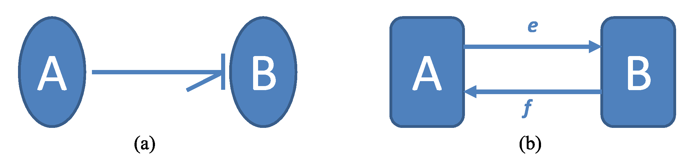
2.1. BG Elements and BG Variables

BG can be denoted as G(N, B), where nodes N represent the BG elements that correspond to energetic physical elements (inertia, resistance and capacitance), source elements (battery, pump, etc.), power/energy constraint BG connecting elements and technological elements (subsystems) and bonds B represent the set of oriented edges that correspond to power/energy exchange among nodal elements. Bond is labeled by two power variables: called flow (f) and effort (e) variables whose product provides the value of physical power flow in that bond. Note that for some energy domains like chemical, the product of these variables on a bond may not be the representation of physical dimension of a power, however it is used for systematically model such energy domains, called pseudo BG model [24,26,33]. All the BG theory obviously remains valid in such cases also.
In Figure 3a, a physical link between subsystem A and subsystem B using the half arrow power bond is presented that represents the direction of energy/power flow among them. In the represented configuration, energy flow is considered towards the destination node B, only when the product of power variables is positive; otherwise, energy flow is in the reverse direction, that is, away from node B. In BG, causality (represented by cross-stroke) is an important structural property that determines the relationship between power/energy variables based on cause and effect analysis. The node which receives the effort information (or gives the flow information), cross-stroke is marked near to that node. For example, according to causality in Figure 3a and corresponding block diagram as in Figure 3b, B receives effort information from A as cross-stroke is marked near B, while A receives flow information from B. In Table 1, various flow and effort variables belonging to different energy domains are shown.
Different systems can be modelled in BG by employing a handful of elements (R, C, I, S f , D f , S e , D e , T F , G Y and J) [34]. Here, R is resistive element (represents dissipation phenomena); I is the inertia element (stores kinetic energy); C is capacitance element (stores potential energy); S f and S e are, respectively, the source of flow and source of effort; D f and D e are, respectively, detectors for flow and effort (virtual sensors); T F is the transformer and G Y is the gyrator. These elements represent the energy transformation between different domains. J represents the junction that accounts for energy conservation laws. It is used to connect the elements based on their interaction with other elements or the sub-systems. Its value is 0 (to connect elements having same effort) and 1 (to connect elements having same flow). R element may also be used as a multi-port resistive-source element (noted R S ) to represent the active resistance that generates entropy. For example, an electric coil that is used for heating acts as a resistance from electricity point of view, but also acts as a source of thermal energy from thermal viewpoint.
The vectorial representation is used to represent the coupling variables of a complex system [26]. The coupled power variables in vectorial form are depicted as:
F = f f l f t h f c h T , E = e f l e t h e c h T ,
where F and E, respectively, are the flow and effort vectors. The suffices f l , t h , c h , respectively, denote the fluidic/hydraulic, thermal and chemical energy domain. Figure 4 shows different ways to illustrate a vector bond.

2.2. Different Levels of Modelling Abstraction

To grasp complex systems, BG technique integrates the different levels of modelling, that is, technological, physical, mathematical and algorithmic levels using the common tool. In technological level, different subsystems of a dynamical system are first identified and then interconnected through energy or power variables. This level is represented by using word BG that shows the architecture of the system in a modularized form. In physical level, the system is modelled in the form of lumped parameters (showing different physical phenomena such as energy storage, dissipation and transformation) using generalized BG elements with power/energy bonds. In mathematical level, dynamical behaviour of the system is represented in the form of mathematical equations such as differential and algebraic equations or in state-space form. The constitutive relations of the constraints and the components of the BG model provide these equations in mathematical form. In algorithmic level, the causal property of BG technique decides how these mathematical equations are algorithmically derived from the graphical BG model. Thus, the structural and causal properties of BG technique enable the dedicated software to systematically and algorithmically obtain the system dynamical equation either in the form of state-space equations or in the form of differential equations for the simulation and analysis purpose. Based on the BG approach, a number of software have been developed and are available for use such as Symbols-Shakti [35] and 20-Sim [36]. In this work, model builder of Symbol-Shakti is used for developing the generic PEM electrolyser model where the structural integrity of different components and sub-systems for the global system modelling is checked. Once the models of different sub-systems (capsules) are built, their corresponding Matlab-Simulink models are systematically derived from implementation point of view.

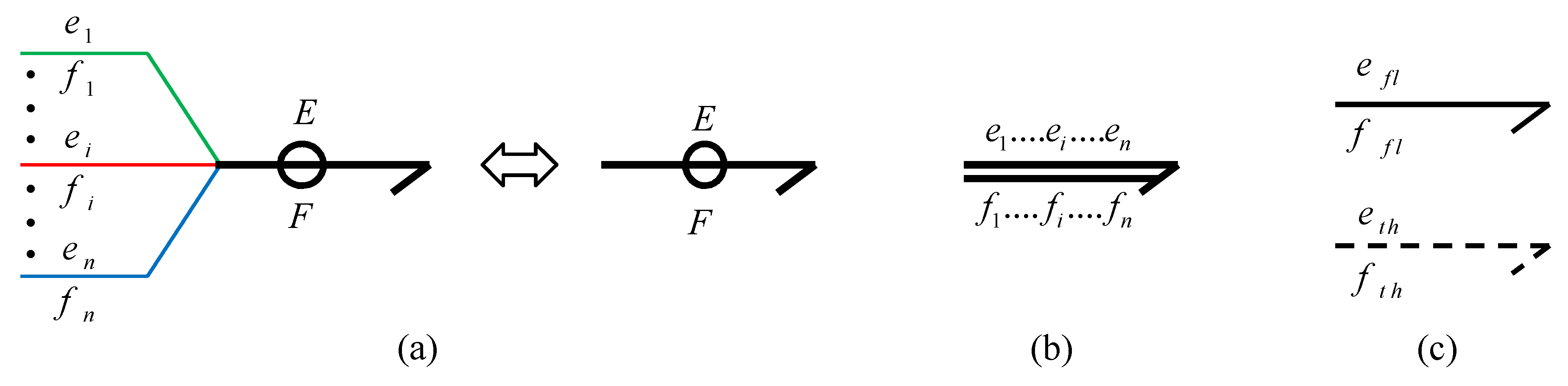
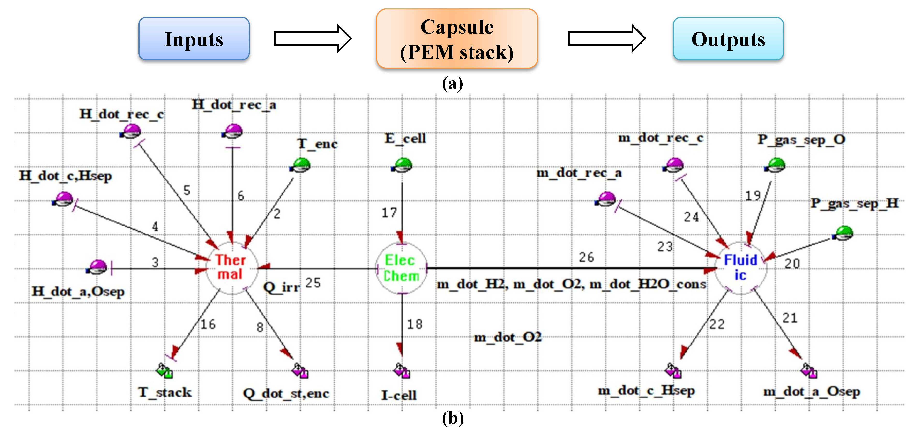
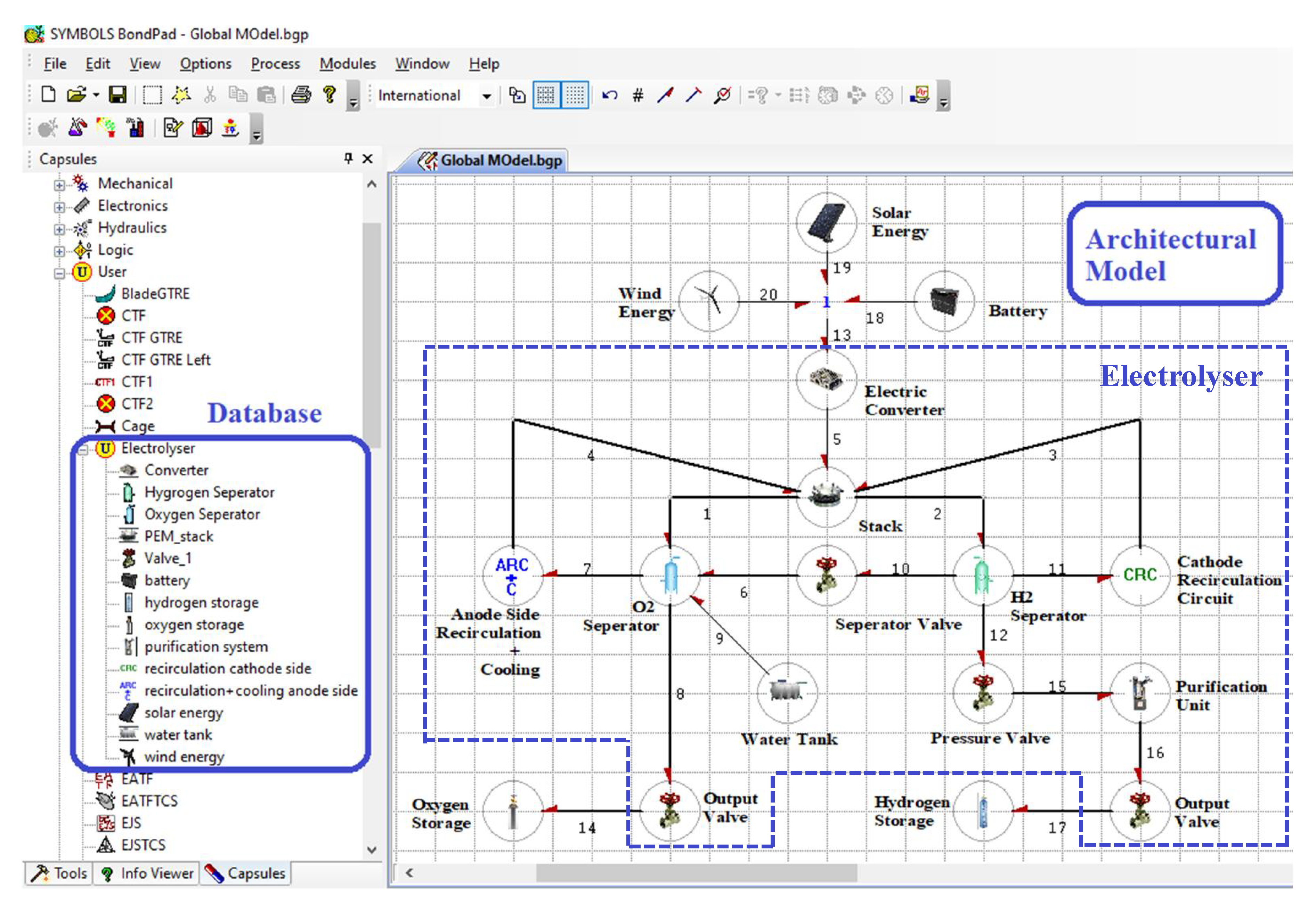
2.3. Modular Building (Capsules)

In Symbols-Shakti, the capsules are properly modelled subsystems that have single or multiple input and output ports. They already have their partially derived equations. When the capsules are assembled to form the complete model, the equations are linked together to form behavioural equations for the complete model. For example, the capsule of PEM stack is developed by coupling the BG sub-models with different energy interactions (electro-chemical, thermal and fluidic). The internal model of the capsule in Symbols-Shakti for a PEM stack is shown in Figure 5.
Depending upon the nature of interaction of the capsules with its environment, the ports can be defined as effort or flow input port and effort or flow output port. Based on the requirements these ports can be attributed as optional and hence are not needed to be connected in order to create the global model. Coupled energy interaction between the sub-models can be represented by a vector bond as shown by bond number 26 in Figure 5. A number of capsules are already available in the database of the software for the commonly used components such as tanks, valves, pipes, heaters and sensors. User defined capsules can be stored in the database and can be used and modified as per the model requirement. Figure 6 shows the user defined capsules, developed for the PEM electrolyser system.

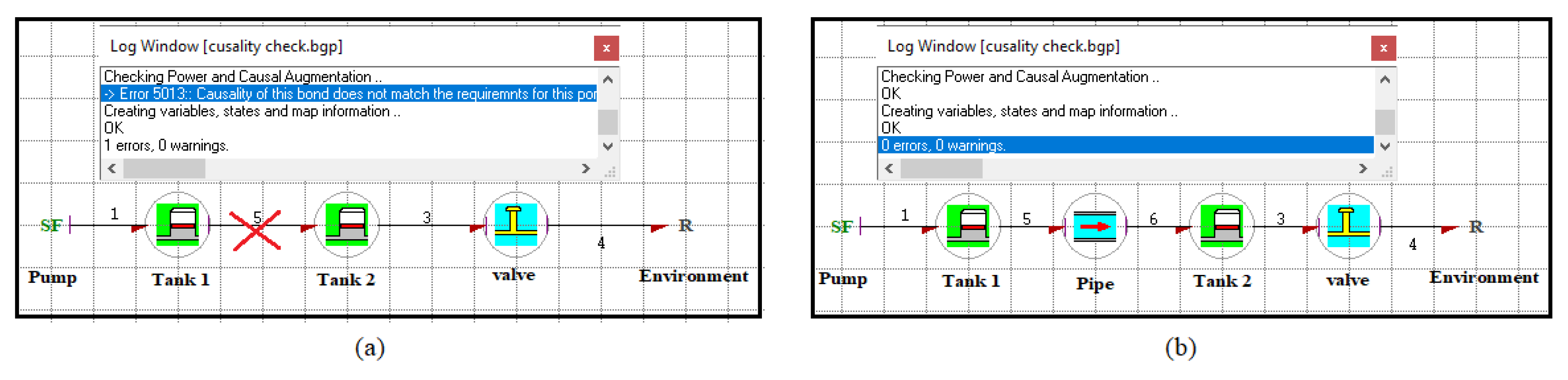
Grammar and Connectivity Rules

Using the capsules, a global model of a complex system can be assembled in the model builder of the Symbols Shakti software. Figure 6 shows the graphical user interface of the model builder. The global model is assembled in the form of piping and instrumentation diagrams using the capsules. For example, the architectural model of a PEM electrolyser is shown in Figure 6. The model builder also generates the behavioural equations for the whole system automatically. To successfully connect the capsules with each other there are certain rules that have to be respected. The connectivity of the capsules is automatically checked by the software for validity. Only the like ports can be connected. The flow (resp. effort) output of a capsule can only be connected to the flow (resp. effort) input of the other capsule and vice versa. For example, Figure 7 demonstrates the requirement of the coherence of causality for the connection of the capsules of two tanks. From Figure 7a, it can be seen that it is not possible to directly connect two tank capsules together as the input for the tank capsule is flow and the output is effort. In order to connect the two tank capsules the resistance of the pipe needs to be considered which takes effort as input and flow as output (as shown in Figure 7b). References [37,38,39] and the reference manual of the software can be referred to for further details.

3. PEM Electrolyser Modelling

In this section, a generic dynamical model of the PEM electrolysis system represented in a modular fashion (in the form of subsystems/capsules) using BG approach is presented. The assumptions taken for the current study are as follow:
  • The cells constituting the stack are identical in nature and connected in series. Thus, the stack with N cells can be modelled as an equivalent single cell that has the same dynamics of the stack.
  • Uniform fluid flows and current distribution are considered between cells.
  • Overpotential due to mass transport or diffusion is negligible with the assumption that PEM system usually operates at low current density.
  • Electrolysis reaction kinetics is assumed firmly as a Faradic process and considers that there is no mass limitation problem in the system.
  • Gases produced are assumed to have similar properties as that of an ideal gas and the partial pressures of these gases are governed by Dalton’s law.
  • Temperature is homogenous throughout the stack.
  • Cell is operated below the boiling temperature of the water.
  • The system parameters are considered as lumped parameters. Pumps and fans are assumed as perfect mass flow sources.

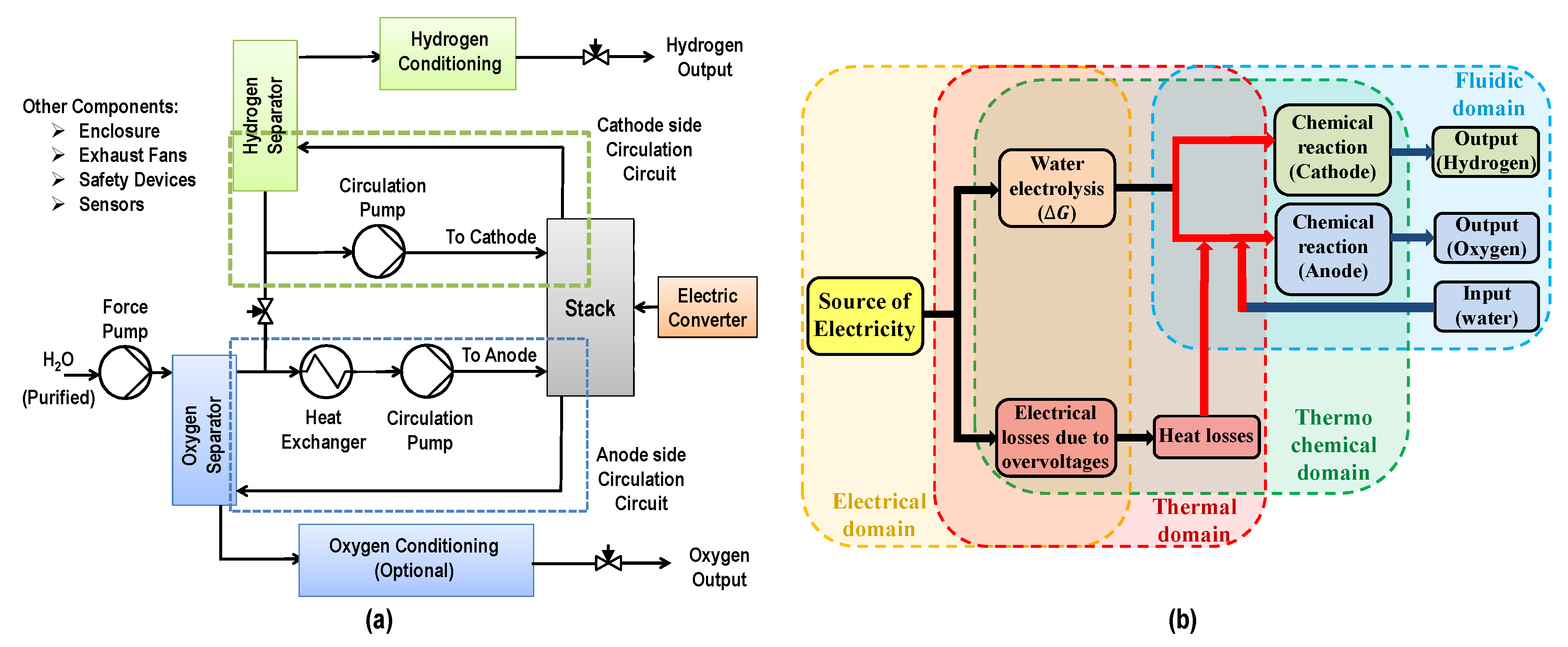
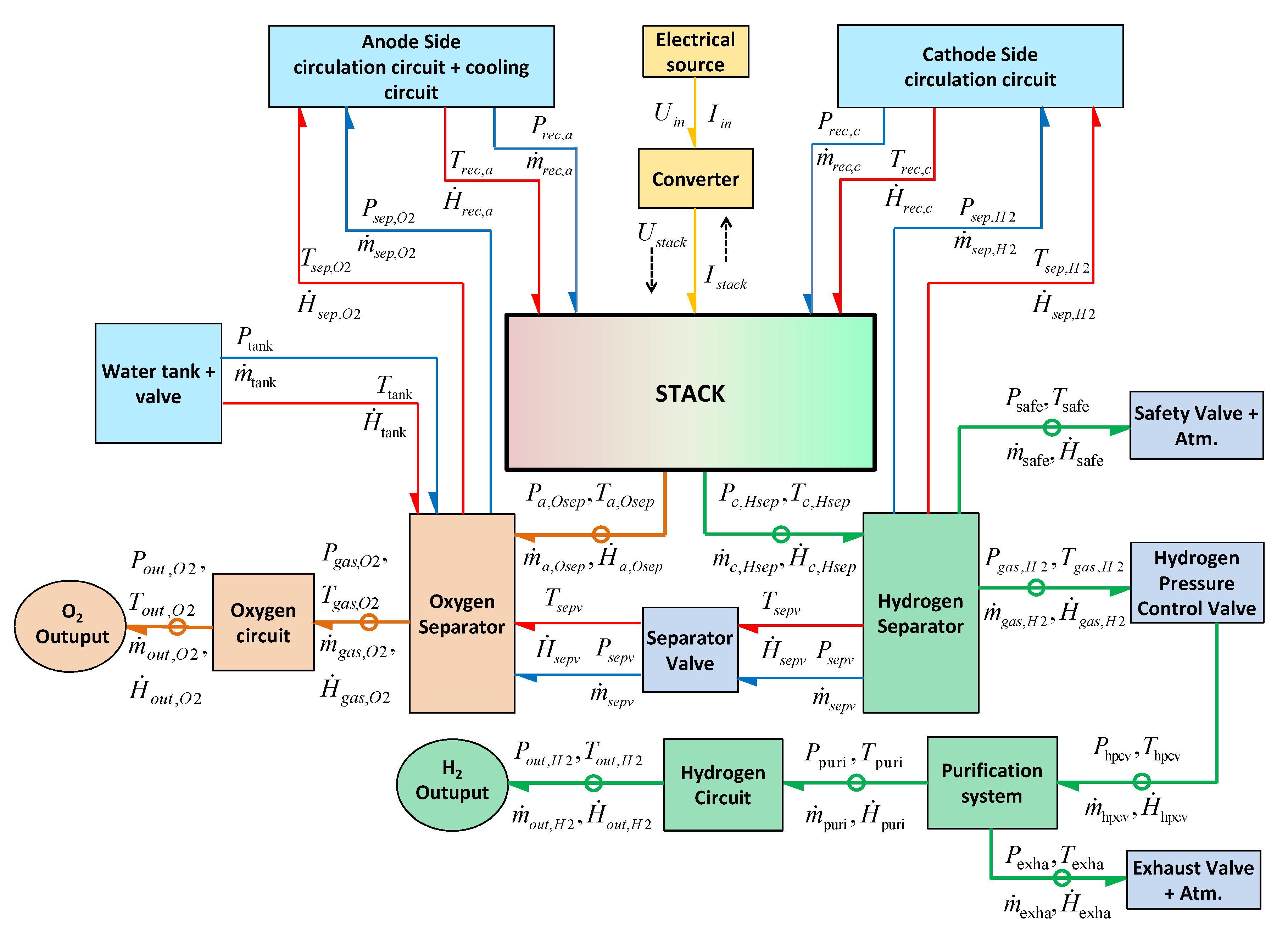
3.1. Technological Representation

The schematic architecture of the PEM electrolyser and the physical variables exchanged between its subsystems are shown by the word BG presented in Figure 8. In Figure 8, line with half arrow represents the power bond, where yellow bonds show the electrical energy (current and voltage variables), red bonds show the thermal energy (heat flow and temperature variables), blue bonds show the fluidic energy (mass flow and pressure variables), green bonds show the thermal-fluidic energy coupling (heat flow, temperature and mass flow, pressure variables) towards hydrogen side. Likewise, orange bonds show the thermal-fluidic energy coupling towards the oxygen side.

3.2. Modular Representation
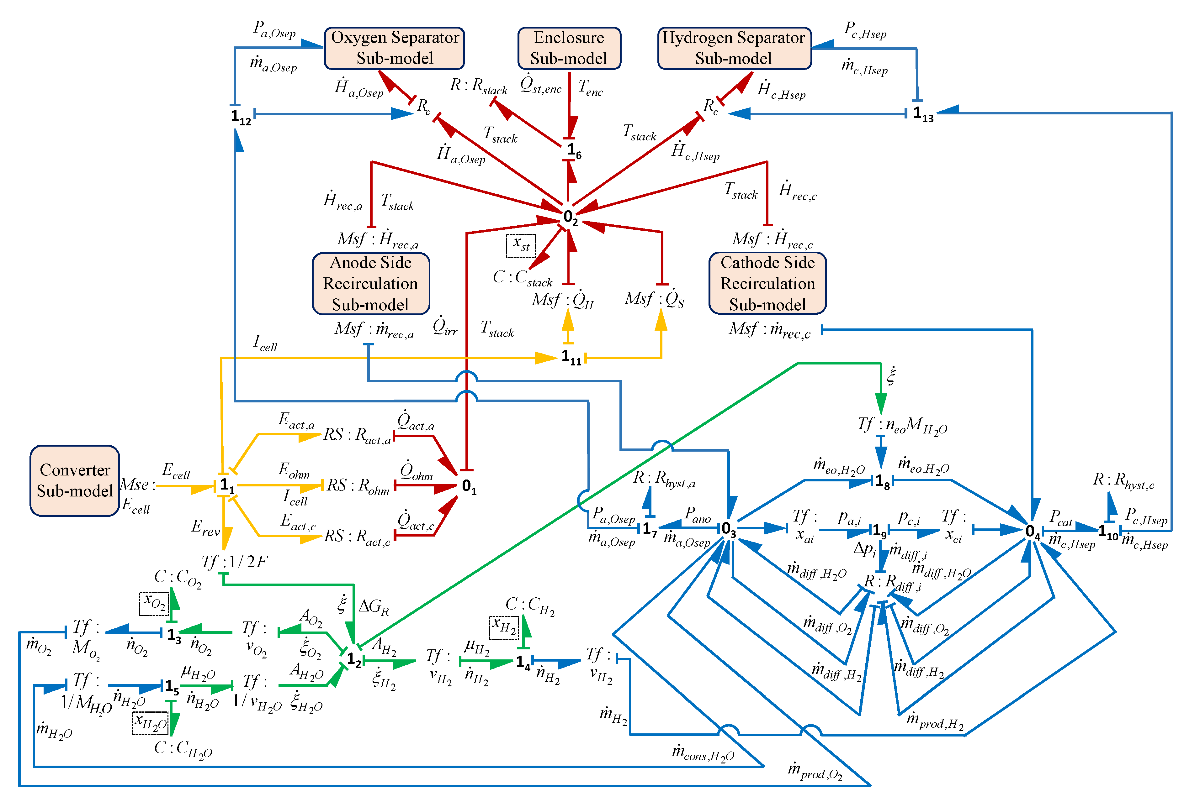
BG capsules are used, from one part, to describe the inner components of the electrolyser, and from another part, to explicit the coupling between the different energies hightlighted by the word BG.

3.2.1. Stack Model

The stack is the heart of the electrolyser. The stack model is the integration of various coupled phenomena which have been modelled as different sub-models to provide more insight.

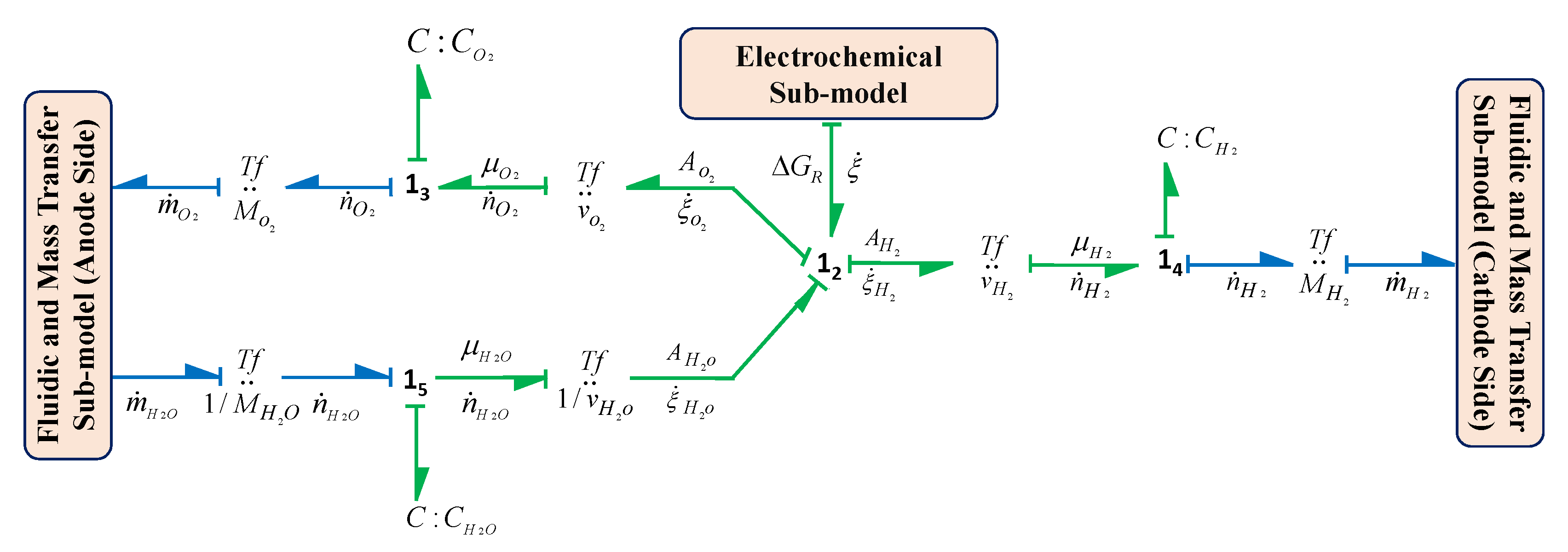
Electrochemical Sub-Model of the Stack

The electrochemical sub-model is one of the crucial sub-models of the electrolysis system. It forms the basis to provide a relation between the cell current and cell voltage at different operating conditions, that is, at different operating pressures and temperatures. The sum of all the electrochemical phenomena leads to a sub-model linking cell voltage and the current density, which is usually represented by a polarization curve. This sub-model explains the real kinetics of the reaction that occurs and gives the information about the amount of product flows according to the water consumed in the electrolysis system and also the production of heat in the stack system. This sub-model considers that electrochemical phenomenon occurs at steady state and thus the sub-model is responded with no time delay which means that there is instantaneous response with respect to change in any input to this sub-model. It is assumed that transient response is very fast and dies out quickly, so it is neglected in model which is also well experimentally demonstrated by the work presented in References [40,41]. The electrochemical BG sub-model in the form of a capsule is shown in Figure 9.
This sub-model can also be used to find the required cell voltage, E c e l l , at any operating condition with respect to reversible potential, E r e v , and different overpotentials which occur due to current flows in the cell results in irreversible heat dissipation. The reason of irreversible heat dissipation in the cell is due to the following: (i) the activation (Faradaic losses) voltages E a c t , a and E a c t , c , respectively, occur at anode-electrolyte and cathode-electrolyte interfaces due to disturbance from the equilibrium chemical reaction and involved activation energies barriers in the preferred reaction. (ii) the electrical ohmic overpotential (non-Faradaic losses) due to internal cell resistance, that is, it is proportional to the current which flows through electrodes, current collectors, bipolar plates and corresponding interconnections between them. Also, this overpotential occurs due to resistance offered by both electrolyte and membrane to the ions flow that separates both the electrodes. Generally, the electrode material in PEM electrolysers has high conductivity, so the flow of electrons is much faster as compared to ionic flow, and thus, usually the ohmic resistance due to ionic transport is considered. (iii) Overpotential due to mass transport or diffusion (non-Faradaic losses). It should be included in the model for a system having higher current density. Nernst equation is used to define the overpotential due to diffusion and it reveals that the diffusion limitation increases with increase in concentration of the product species at the reaction interface [42].
In this sub-model, E c e l l is modelled as a modulated source of effort BG element, that is, M s e : E c e l l and all the overpotentials are modelled by generalized R S coupled resistive elements as R S : R a c t , a , R S : R a c t , c and R S : R o h m corresponding to anodic activation resistance, cathodic activation resistance and ohmic resistance, respectively. Here, the generalized R S coupled resistance element shows the coupled energy dynamics and links the electrical domain with the thermal domain. It acts as a source and transmits the generated heat or entropy to the thermal domain due to the current flow in electrical domain [26,43]. Also, the transformation of electrical energy into chemical energy and vice a versa is modelled by transformer T f generalized BG element, which describes the Faraday’s law by linking the rate of reaction flow ( ξ ˙ ) with the current flow through cell ( I c e l l ), number of moles of electron transferred n (here n = 2 ) and Faraday’s constant F; and, also by linking reversible cell voltage ( E r e v ) with free energy of water dissociation Δ G R , n and F, which are represented in Equations (3) and (4).
ξ ˙ = I c e l l n × F
E r e v = Δ G R n × F .
Here E r e v is the reversible potential which is the minimum potential required for the electrolysis reaction. As per Reference [2], the reversible potential E r e v is expressed as in Equation (5) at any operating temperature and pressure condition.
E r e v = E r e v 0 + R × T 2 F ln p H 2 × p O 2 1 / 2 a H 2 O ,
where E r e v 0 is the standard reversible cell potential at standard operating conditions (at standard temperature and pressure), R is the ideal gas constant, p i is the partial pressure of the i t h species and a H 2 O is the chemical activity of water. The E r e v 0 is usually temperature dependent and is empirically defined as [2,23,44,45]
E r e v 0 = 1.5184 1.5421 × 10 3 T + 9.523 × 10 5 T × ln T + 9.84 × 10 8 T 2 .
Activation overpotential: There is a relation between the kinetic part of the reaction, that is, the current density, with the thermodynamic part, that is, the overpotential. At equilibrium current exchange density ( J 0 ) is defined and it is related with the exponential function of negative free Gibbs energy at equilibrium ( Δ G 0 ). The value of the parameter J 0 or Δ G 0 should be obtained from the experiment. For the electrolysis process, that is, possibility of occurring the dissociation of water, the cell voltage is usually more than the reversible standard voltage which results in overpotential because of current flow, and thus, it contributes to polarization. This current flow is usually the difference between anodic and cathodic currents at the non-equilibrium condition. The relation between the actual current and the overpotential is usually obtained by using Buttler-Volmer equation as given in Equation (7) and used in much of the literature [14,17,44,46,47].
J c e l l = J 0 , k × exp α k × n × F R × T × E a c t , k exp ( 1 α k ) × n × F R × T × E a c t , k ,
where J c e l l = I c e l l / A M is current density of cell, A M is cross-sectional area of membrane. Also, J 0 , k and α k represent the current exchange density and charge transfer or symmetry factor coefficient, respectively, at anode or cathode. Usually, symmetry factor is taken as 0.5; however it lies between 0 and 1. Thus, at α k = 0.5 , the overpotential E a c t , k at anode or cathode can be expressed by Equation (8).
E a c t , k = R × T F sin h 1 J c e l l 2 J 0 , k .
In thermochemical model (Figure 9), Equation (8) is the constitutive relation for nonlinear resistive element R S : R a c t , k . The parameter J 0 , k for each electrode is expressed as
J 0 , k = J 0 , k r e f × exp Δ G 0 , k R × T ,
where J 0 , k r e f and Δ G 0 , k are obtained from the experimental data using model fitting technique and the temperature T is obtained from the thermal model of the stack.
Ohmic overpotential: This overpotential is modelled by the dissipative element, that is, generalized BG resistive element R : R o h m . According to the resistive causality in the BG sub-model (Figure 9), the constitutive relation for R : R o h m is given as
I c e l l = E o h m R o h m ,
where E o h m is the ohmic overpotential. The ohmic resistance R o h m mainly includes the resistance offered by the membrane to ions flow and also includes the other ohmic resistance R o t h e r offered by the internal cell components except the membrane. Thus, R o h m is obtained from Equation (11) that depends upon the properties ( σ M ) and parameters of the membrane ( L M , A M ) . σ M represents the membrane conductivity, L M and A M , respectively, represent the length and cross-sectional area of the membrane. Moreover, the resistance R o t h e r can be obtained from the experiments using model fitting technique.
R o h m = d M σ M + R o t h e r ,
where d M is the ratio of L M to A M and σ M can be empirically defined as in Equation (12). Membrane conductivity depends on cell temperature T and the membrane water content parameter γ .
σ M = ( 0.005139 γ 0.00326 ) × e x p 1268 × 1 303 1 T .
The parameter γ value varies from 14 to 25, whose value depends on the nature of membrane hydration. For a poorly hydrated membrane, it is taken as 14 while for fully hydrated it is taken as 25 [42].
Based on BG causal properties and constitutive relations for different elements, different relations can be systematically obtained from the sub-model of electrochemical phenomenon. At junction 1 1 (refer Figure 9), the conservative phenomenon can be written as in Equation (13):
( e 1 × f 1 ) ( e 2 × f 2 ) ( e 3 × f 3 ) ( e 4 × f 4 ) ( e 5 × f 5 ) = 0 .
Since, at junction 1 1 all the flows are equal, that is, f 1 = f 2 = f 3 = f 4 = f 5 . Thus, as per causality in sub-model (Figure 9), e 3 = E o h m can be obtained from Equation (13) as
E o h m = e 1 e 2 e 4 e 5 ,
where value of e 1 = E c e l l , e 2 = E a c t , a , e 4 = E a c t , c , e 5 = E r e v . So, Equation (14) becomes
E o h m = E c e l l E a c t , a E a c t , c E r e v ,
where E c e l l is derived from BG source element M s e : E c e l l as input causality. E a c t , a , E a c t , c are derived from constitutive relations for BG elements R S : R a c t , a , R S : R a c t , c as in Equation (8) and E r e v is obtained from T f : 1 / 2 F as in Equation (4) or (5). Thus, using BG submodel, E o h m can be systematically derived as
E o h m = E c e l l R × T F sin h 1 J c e l l 2 J 0 , a R × T F sin h 1 J c e l l 2 J 0 , c E r e v 0 R × T 2 F ln p H 2 × p O 2 1 / 2 a H 2 O .
Thus, using Equation (10), the cell current I c e l l can be derived from the electrochemical BG submodel by using constitutive relation for R : R o h m , which is used for controlling the hydrogen production by the cell. The required input cell voltage can also be derived by rearranging the Equation (16)
E c e l l = E o h m + R × T F sin h 1 J c e l l 2 J 0 , a + R × T F sin h 1 J c e l l 2 J 0 , c + E r e v 0 + R × T 2 F ln p H 2 × p O 2 1 / 2 a H 2 O .
Likewise, using the property of junction 0 1 (refer Figure 9), the conservative phenomenon can be written as
( e 6 × f 6 ) + ( e 7 × f 7 ) + ( e 8 × f 8 ) ( e 9 × f 9 ) = 0 .
Since, at junction 0 1 all the efforts are equal, that is, e 6 = e 7 = e 8 = e 9 . Thus, as per causality in sub-model (Figure 9), f 9 = Q ˙ i r r can be obtained from Equation (18) as
Q ˙ i r r = f 6 + f 7 + f 8 ,
where value of f 6 = Q ˙ a c t , a , f 7 = Q ˙ o h m , f 8 = Q ˙ a c t , c . So, Equation (19) becomes
Q ˙ i r r = Q ˙ a c t , a + Q ˙ o h m + Q ˙ a c t , c ,
where Q ˙ i r r denotes the irreversible heat flow which is systematically derived from BG submodel and obtained as the summation of activation losses at anode, cathode and ohmic loss.

Chemical-Fluidic Sub-Model of the Stack

In chemical-fluidic sub-model, the amount of hydrogen and oxygen production rates can be predicted with respect to consumed water. The BG chemical-fluidic sub-model in the form of a capsule is shown in Figure 10.
In the sub-model, transformers T f : ν i and T f : M i generalized BG elements are used to find the rate of production of the products with respect to consumed reactant. Also, C : C i represent the storage of the matter for the i t h species. The rate of produced mass for the i t h species, that is, m ˙ i , is obtained from the rate of reaction flow ξ ˙ from Equation (21) as
m ˙ i = ν i × M i × ξ ˙ = ν i × M i × I c e l l n × F ,
where ν i and M i , respectively, denote the coefficient of stoichiometry and molar mass of i t h species.

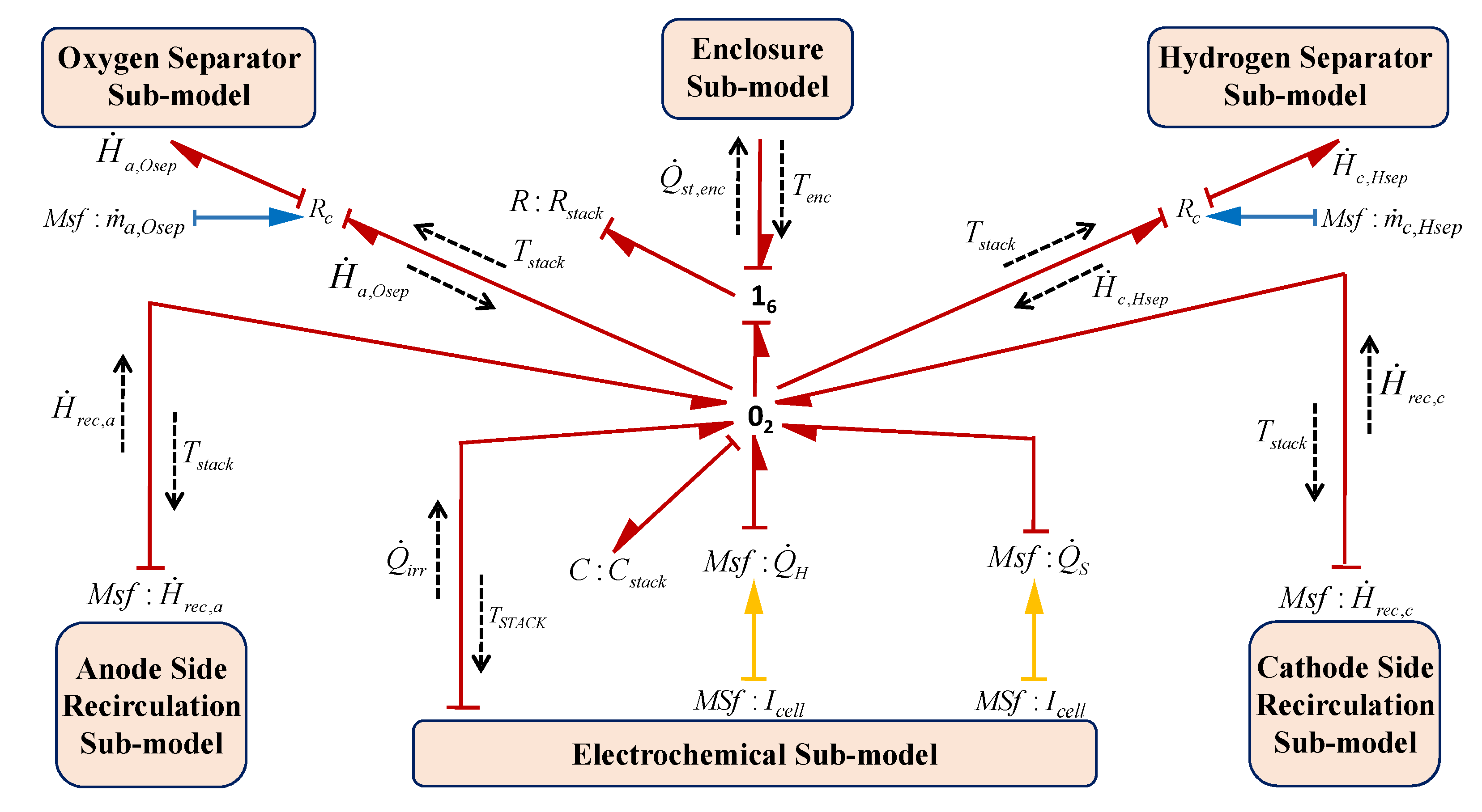
Thermal Sub-Model of the Stack

Thermal sub-model predicts the dynamic behaviour of the temperature evolution inside the stack which ultimately affects the relation between cell current and voltage. Thus, durability and efficiency of the electrolysis system is also affected. The complete thermal BG sub-model in the form of a capsule is represented in Figure 11. The sub-model considers the major contribution of the heat from the different sources and phenomena such as heat input to stack by the water inflow towards anode and cathode side, heat taken away by the water outflow from stack towards hydrogen and oxygen separators, thermodynamics of chemical components during reaction (dissociation of water and production of gases) or endothermic nature of chemical reaction, Joule effect phenomenon due to circulation of charge/current, heat due to entropy change in reaction, thermal activated phenomenon due to mass transfer and diffusion and thermal effects due to system enclosure temperature.
This thermal sub-model is considered as a first order nonlinear model having one dynamic generalized BG capacitance C element. Here generalized C : C s t a c k element, considered as a constant lumped parameter, models the thermal capacitance of the stack, and thus, it is assumed that temperature is homogenous throughout the stack. This lumped parameter can be estimated from the experiment using model fitting technique. From the BG thermal sub-model, the temperature of stack using constitutive relation of C : C s t a c k and junction 0 2 is obtained as
T s t a c k = 1 C s t a c k H ˙ r e c , a + H ˙ r e c , c + Q ˙ i r r + Q ˙ H + Q ˙ S H ˙ a , O s e p H ˙ c , H s e p Q ˙ s t , e n c d t .
In Equation (22), H ˙ r e c , a , H ˙ r e c , c and H ˙ a , O s e p , H ˙ c , H s e p respectively, represent the enthalpy rate due to water inflow from recirculation circuit towards anode side, cathode side and water outflow from the stack towards oxygen and hydrogen separator side. These enthalpy flows are related with the molar enthalpy H i and molar flow rate n ˙ i of the involved species in the reaction. Q ˙ i r r is irreversible heat flow due to activations and ohmic losses, Q ˙ H that is , Q ˙ H = ( I c e l l × Δ H R ) / ( 2 F ) denotes heat flow rate due to chemical components during reaction or endothermic nature of reaction (dissociation of water and production of gases), Q ˙ S that is , Q ˙ S = ( I c e l l × Δ S R ) / ( 2 F ) denotes the heat flow rate due to entropy change and Q ˙ s t , e n c denotes heat transfer from stack to system enclosure due to temperature difference.

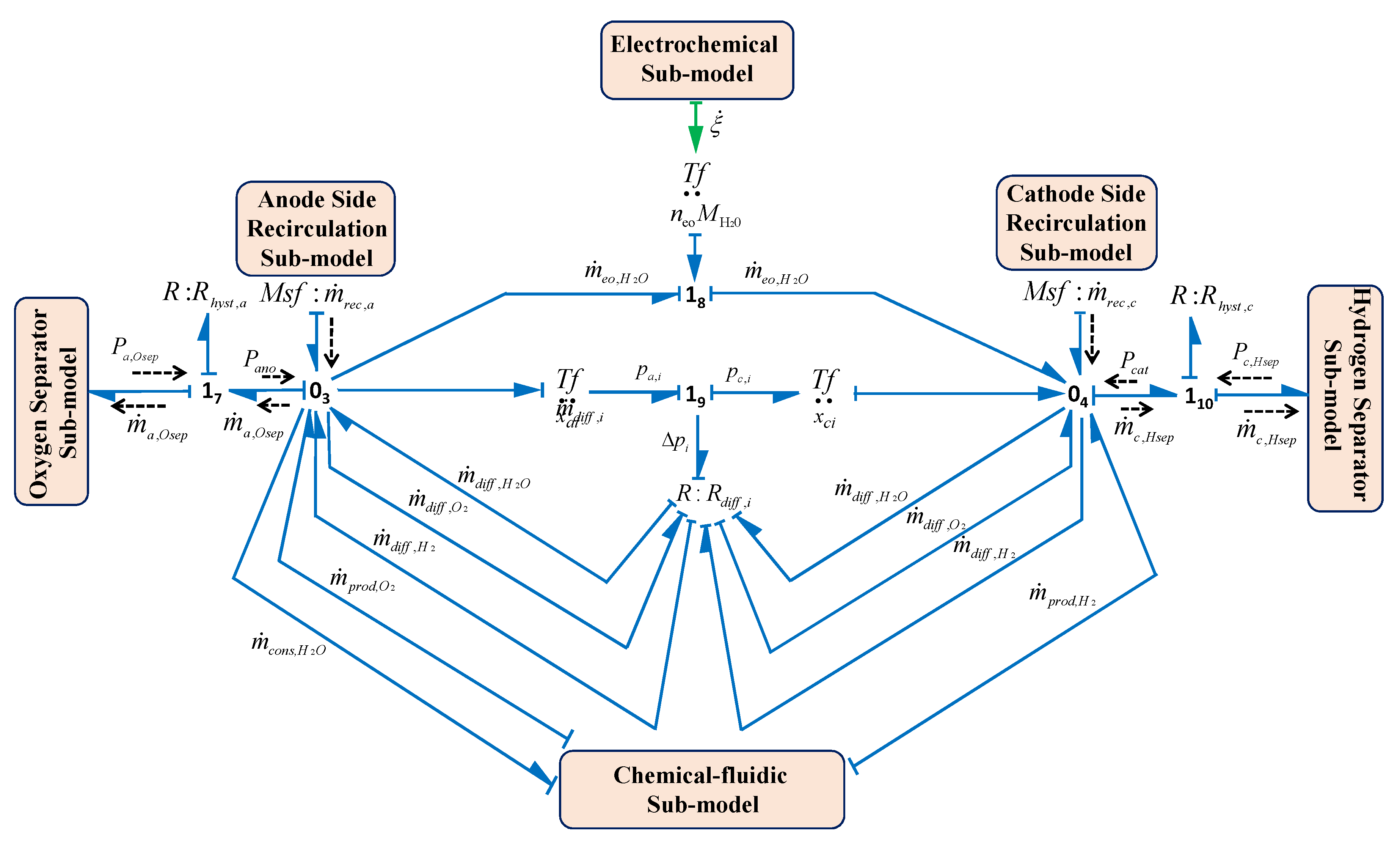
Fluidic and Mass Transfer Sub-Model

The global behaviour and the efficiency of cell can be affected due to the phenomena of fluidic motion and mass transfer and these cannot be ignored while developing the model of the electrolysis system. Thus, the phenomenon of fluidic motion and mass transfer must be integrated within thermal and electrochemical sub-models. It is assumed that there is no accumulation of fluid inside the stack and the product produced is continuously evacuated from the stack. This sub-model includes the transfer of water from anode to cathode by considering the electro-osmosis phenomenon and also considers the transfer in reverse direction, that is, from cathode to anode, by the process of diffusion. This sub-model also includes the crossover of produced gases, that is, oxygen and hydrogen gas flows towards the opposite electrode with respect to the electrode where they produce. The BG sub-model of fluidic and mass transfer phenomenon in the form of a capsule is shown in Figure 12.
In this sub-model, resistive BG field element R : R d i f f , i , that is, R : R d i f f , H 2 O , R : R d i f f , O 2 , R : R d i f f , H 2 , and transformer element T f : n e o M H 2 O are used, respectively, to model the crossover or diffusion flows due to water diffusion, oxygen diffusion, hydrogen diffusion and electro-osmosis diffusion. R H y s t , a and R H y s t , c are the hydraulic resistances at anode and cathode side, respectively. Thus, the model provides the output mass flow of the mixture from the stack at the anode and cathode sides using constitutive relation of junction 0 3 and 0 4 as given by Equations (23) and (24), respectively.
m ˙ a , O s e p = m ˙ r e c , a + m ˙ p r o d , O 2 m ˙ c o n s , H 2 O m ˙ e o , H 2 O + m ˙ d i f f , H 2 + m ˙ d i f f , H 2 O m ˙ d i f f , O 2
m ˙ c , H s e p = m ˙ r e c , c + m ˙ p r o d , H 2 + m ˙ e o , H 2 O + m ˙ d i f f , O 2 m ˙ d i f f , H 2 O m ˙ d i f f , H 2 ,
where m ˙ r e c , a , m ˙ r e c , c , respectively, denote rate of inflow masses from recirculation circuit to anode and cathode side. m ˙ p r o d , O 2 , m ˙ p r o d , H 2 and m ˙ c o n s , H 2 O , respectively, denote production of oxygen, hydrogen and water consumed which are obtained from electrochemical model. Also, m ˙ e o , H 2 O denotes the rate of water mass flow due to electro-osmosis, however, this phenomenon does not depend on thickness of the membrane. The electro-osmosis flow, m ˙ e o , H 2 O , mainly depends on the magnitude of electric current flow during electrolysis process and the number of dragged water molecules by a proton ion as given in Equation (25). This number is denoted by n e o and called as electro-osmosis coefficient [44,48]. This flow, m ˙ e o , H 2 O , is obtained by using the generalized transformer element T f : n e o M H 2 O in the fluidic model which is coupled with the rate of reaction ξ ˙ of the thermochemical model.
m ˙ e o , H 2 O = n e o × M H 2 O × ξ ˙ = n e o × M H 2 O × I c e l l n × F .
Also, m ˙ d i f f , i denotes the flow of diffusion for the i t h species through membrane and this flow for i t h species is obtained from the constitutive relation of the generalized resistive element R : R d i f f , i . This sub-model shows that the diffusion flow for the i t h species is proportional to the change in partial pressure at the both side of the membrane Δ p i and also the resistance R d i f f , i depends on the length of membrane L M , diffusion parameter D i and the Henry’s parameter H i [49,50] as represented in Equations (26) and (27), respectively.
m ˙ d i f f , i = Δ p i × sign p i p j R d i f f , i
R d i f f , i = H i × L M D i × M i × A M .
Thus, the global stack model, as shown in Figure 13, is obtained by integrating all the sub-models (capsules) such as electrochemical, chemical-fluidic, thermal, fluidic and mass transfer sub-models.
The state-space equation for the stack can now be derived systematically and automatically from the BG sub-model of the stack (shown in Equation (28)),
x ˙ O 2 x ˙ H 2 x ˙ H 2 O = v o 2 2 4 F 2 × R o h m × C O 2 v O 2 × v H 2 4 F 2 × R o h m × C H 2 v O 2 × v H 2 O 4 F 2 × R o h m × C H 2 O v H 2 × v O 2 4 F 2 × R o h m × C O 2 v H 2 2 4 F 2 × R o h m × C H 2 v H 2 × v H 2 O 4 F 2 × R o h m × C H 2 O v H 2 O × v O 2 4 F 2 × R o h m × C O 2 v H 2 O × v H 2 4 F 2 × R o h m × C H 2 v H 2 O 2 4 F 2 × R o h m × C H 2 O x O 2 x H 2 x H 2 O + v O 2 2 F × R o h m × 1 R a c t , a R o h m R a c t , c R o h m 0 0 0 0 0 v H 2 2 F × R o h m × 1 R a c t , a R o h m R a c t , c R o h m 0 0 0 0 0 v H 2 O 2 F × R o h m × 1 R a c t , a R o h m R a c t , c R o h m 0 0 0 0 0 E c e l l m ˙ r e c , a m ˙ r e c , c P a , O s e p P c , H s e p T e n c x ˙ s t = f t , x O 2 , x H 2 , x H 2 O , E c e l l , m ˙ r e c , a , m ˙ r e c , c , P a , O s e p , P c , H s e p , T e n c ,
where x O 2 , x H 2 , x H 2 O and x s t are the states of the stack and function f shows the non linear relation for the state x s t . Similarly, the state-space equations for the complete model and each sub-model can also be generated for developing control algorithms.
Further, BG modelling of other subsystems and components as prescribed in word BG (see Figure 8) such as: electrical converter, hydrogen and oxygen separator vessels, heat exchanger, cooling and recirculation systems, purification system, the pneumatically controlled hydraulic valves and the stack enclosure, is required for the complete modelling and dynamical study of the electrolysis system.

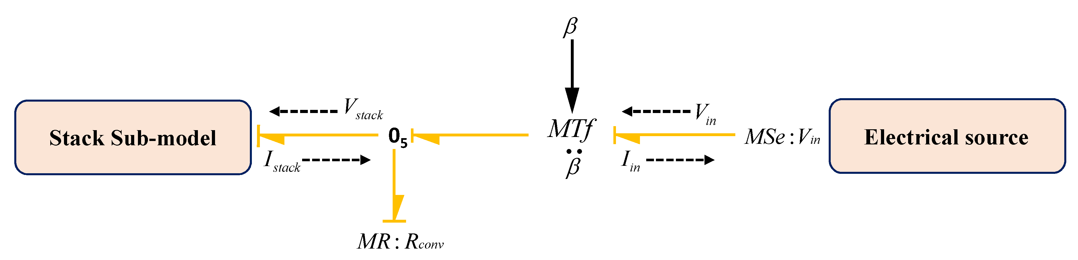
3.2.2. Converter Sub-Model

Converter provides the control power input to the stack according to the operational point of the electrolyser. Usually, converter has a very fast response time (less than 0.1 s); thus, the dynamic model of the converter has instantaneous power output. This sub-model is shown in Figure 14.
Here, physical phenomena of the converter is modelled by using a modulated transformer ( M T f : β ) and resistive ( R : R c o n v ) generalized BG elements. In the model, M s e : V i n is the input voltage to the converter from the electrical source (solar and/or wind source) and V s t a c k is the output of the converter which is fed in to the electrolyser for water dissociation. Thus, using dynamic BG sub-model (Figure 14), constitutive relations can be derived as
V s t a c k = β × V i n
P i n = P s t a c k + P c o n v
P c o n v = P i n × 1 ε c o n v ,
where β is the coefficient of transformer, P i n = V i n × I i n denotes input power, P s t a c k = V s t a c k × I s t a c k denotes output power from the converter which is input to the stack, P c o n v denotes the dissipation power of the converter due to its internal resistance and ε c o n v denotes converter efficiency.

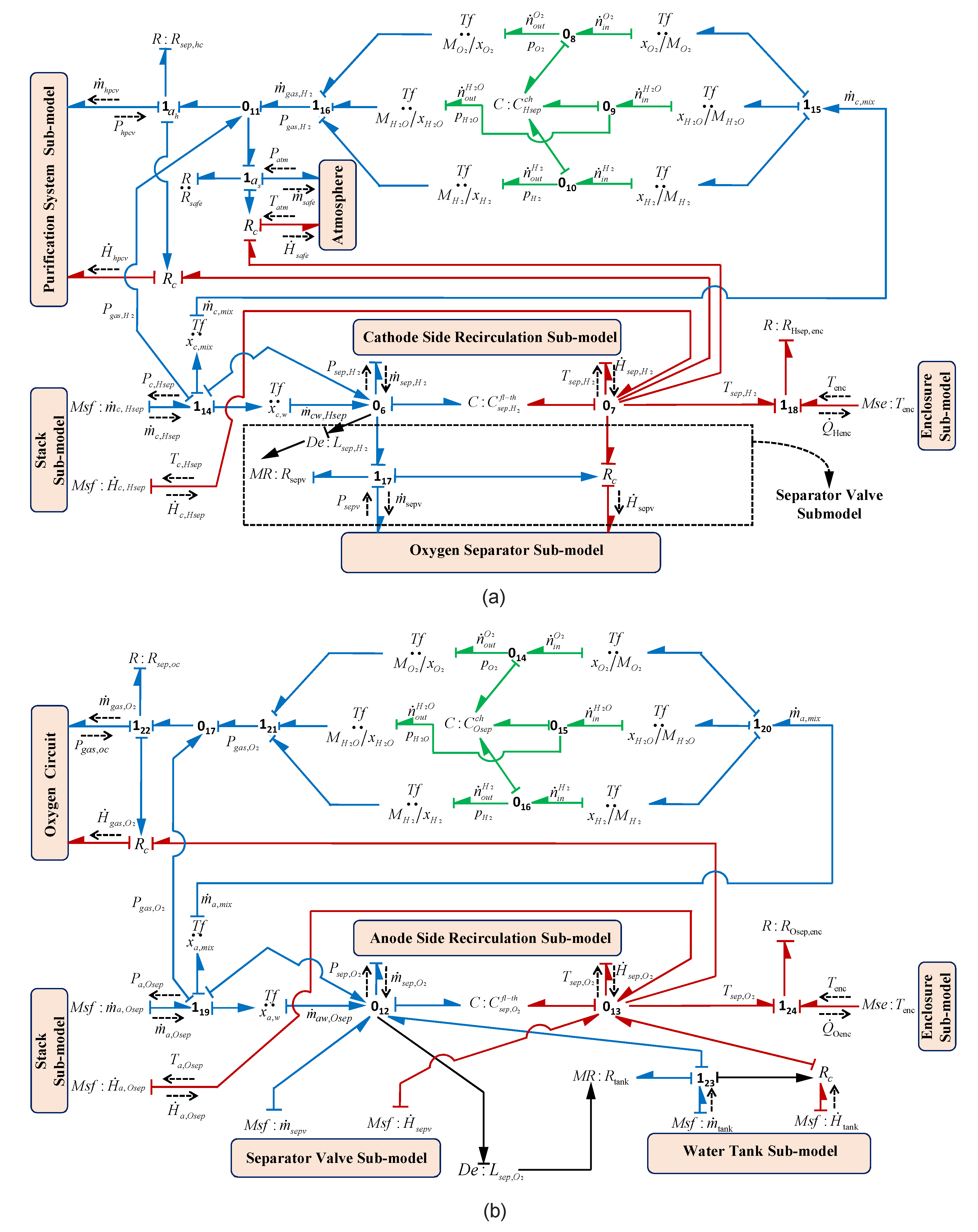
3.2.3. Separator Sub-Models

Usually gas is collected over water in a vessel and due to the light weight of the gas it goes up and can be separated from the water. When the gas pressure reaches a certain fixed preset value in the separator it comes out from the separator vessel to the storage tank. In the electrolysis system, two separators are used for gas liquid separation: (i) hydrogen separation and (ii) oxygen separation. The separator subsystem includes the interaction of fluidic, thermal and chemical phenomena. In the modelling of each separator, it is assumed that the vessel is in cylindrical shape having a cross-sectional area A s e p , i . The BG sub-models of the hydrogen and oxygen separators are shown in Figure 15a,b, respectively.
Separator fluidic Phenomena: The hydraulic pressures or the water levels in the Hydrogen Separator Vessel (HSV) and Oxygen Separator Vessel (OSV) are determined from the continuity equations and these phenomenons are modelled in the sub-models as in Figure 15a,b, respectively.
The hydraulic capacity as a lumped parameter for i t h separator ( i = H 2 , O 2 ) is denoted by C s e p , i f l = A s e p , i / g , where g is gravity. First the entire phenomena are discussed for HSV, and then likewise these are presented for OSV. Thus, for HSV from Figure 15a, using constitutive relation of C : C s e p , H 2 f l and junction 0 6 , HSV pressure can be obtained as
P s e p , H 2 = 1 C s e p , H 2 f l m ˙ c w , H s e p m ˙ s e p v m ˙ s e p , H 2 d t ,
where P s e p , H 2 = ρ w × g × L s e p , H 2 is water pressure in HSV, L s e p , H 2 is water level in HSV, ρ w is water density, m ˙ c w , H s e p is the water mass flow which is the product of known mass fraction of water x c , w and the mass flow of mixture, m ˙ c , H s e p (obtained in Equation (24)), m ˙ s e p v is the water mass flow from the HSV to OSV through the separator valve (modelled using modulated resistive element M R : R s e p v ). The sub-model of the separator valve [39] is highlighted in the Figure 15a. m ˙ s e p , H 2 is the water mass flow out from the HSV to cathode side recirculation circuit.
Separator thermal Phenomena: The thermal capacity of the vessel is modelled by using lumped parameter, C : C s e p , i t h , whose value depends on cross-sectional area A s e p , i and water level L s e p , i in the vessel. Also, it is assumed that the coefficient of heat transfer of the vessel is constant. Thus, for HSV from Figure 15a, using constitutive relation of C : C s e p , H 2 t h and junction 0 7 , HSV temperature can be obtained as
T s e p , H 2 = 1 C s e p , H 2 t h H ˙ c , H s e p H ˙ s e p v H ˙ s e p , H 2 H ˙ h p c v H ˙ s a f e Q ˙ H e n c d t ,
where T s e p , H 2 temperature inside HSV, H ˙ c , O s e p is the enthalpy flow of the water and gas mixture from the cathode side of the stack to HSV and H ˙ s e p , H 2 is the enthalpy flow out from the HSV to cathode side recirculation circuit and Q ˙ H e n c is the rate of heat loss due to temperature gradient between HSV and system enclosure. Note that all the enthalpy flow is correlated with their respective mass flow of water and mixture. The value of the enthalpy flows H ˙ g a s , i and H ˙ j coupled with mass flows m ˙ g a s , i and m ˙ j ( i = O 2 , H 2 ; j = t a n k ) can be obtained from the expression as presented in Equations (34) and (35), respectively. This coupling between thermal and fluidic phenomena is represented by generalized R c element.
H ˙ g a s , i = m ˙ g a s , i × i C p i × T g a s , i
H ˙ j = m ˙ j × C p j × T j ,
where C p j and i C p i , respectively, denote specific heat constant of water and gas. The thermal loss, Q ˙ H e n c , is modelled by generalized BG resistive element R : R H s e p , e n c . Also, the system enclosure temperature is modelled as BG modulated source of effort element as M s e : T e n c , which is obtained from the thermal sub-model of the enclosure. Moreover, generalized detector element D e : L s e p , H 2 is used which shows the measurement of separator water level that is further utilized by the controller for controlling the percentage opening of separator valve as per level set value.
Separator chemical Phenomena: For calculation of partial pressure, P H s e p , i c h , of the i t h species, the chemical capacitance is modelled by using lumped parameter, C : C H s e p , i c h at cathode side separator, whose value depends on molar mass M i , volume V H s e p , i of the i t h species, temperature T H s e p , i and the gas constant R which is obtained from Equation (36).
C H s e p , i c h = M i × V H s e p , i R × T H s e p , i .
Thus, for HSV from Figure 15a, using constitutive relation of C : C H s e p , i c h and junction 0 8 / 0 9 / 0 10 , gases partial pressures can be obtained as
P H s e p , i c h = 1 C H s e p , i c h n ˙ c i d t = 1 C H s e p , i c h m ˙ c , H s e p × x c , m i x × x c , i M i m ˙ g a s , H 2 × x c , i M i d t ,
where n ˙ c i denotes gas mass flow rate at cathode side, x c , i and x c , m i x , respectively, denote mass fraction of i t h species and gas mixture (hydrogen, oxygen and water vapor) leaving from cathode side of stack to HSV, m ˙ g a s , H 2 is the output gas flow towards purification system. The total pressure P s e p , H 2 of the oxygen separator can be obtained from the summation of all the partial pressures of the gases according to Dalton’s law. The valve and the pipe resistances are modelled using R elements.
Likewise, the fluidic, thermal and chemical phenomena for the OSV can be represented by Equations (38)–(40), respectively. For OSV from Figure 15b, using constitutive relation of C : C s e p , O 2 f l and junction 0 12 , OSV pressure can be obtained as can be written as
P s e p , O 2 = 1 C s e p , O 2 f l m ˙ t a n k + m ˙ s e p v + m ˙ a w , O s e p m ˙ s e p , O 2 d t ,
where P s e p , O 2 = ρ w . g . L s e p , O 2 is water pressure in OSV, L s e p , O 2 is water level in OSV, m ˙ t a n k is the water mass flow from water tank to OSV. m ˙ a w , O s e p is the water mass flow from the anode side of the stack to OSV and m ˙ s e p , O 2 is the water mass flow out from the OSV to anode side recirculation circuit. The water mass flow m ˙ a w , O s e p can be obtained using the product of known mass fraction of water x a , w and the mass flow of mixture, m ˙ a , O s e p , obtained in Equation (23).
For OSV from Figure 15b, using constitutive relation of C : C s e p , O 2 t h and junction 0 13 , OSV temperature can be obtained as
T s e p , O 2 = 1 C s e p , O 2 t h H ˙ t a n k + H ˙ s e p v + H ˙ a , O s e p H ˙ s e p , O 2 H ˙ g a s , O 2 Q ˙ O e n c d t ,
where T s e p , O 2 temperature inside OSV, H ˙ t a n k is the enthalpy flow from water tank to OSV, H ˙ s e p v is the enthalpy flow from the HSV to OSV through the separator valve, H ˙ a , O s e p is the enthalpy flow of the water and gas mixture from the anode side of the stack to OSV and H ˙ s e p , O 2 is the enthalpy flow out from the OSV to anode side recirculation circuit, H ˙ g a s , O 2 is the heat flow output from OSV towards oxygen circuit and Q ˙ O e n c is the rate of heat loss due to temperature gradient between OSV and system enclosure.
For OSV from Figure 15b, using constitutive relation of C : C H s e p , i c h and junction 0 14 / 0 15 / 0 16 , gases partial pressures can be obtained as
P O s e p , i c h = 1 C O s e p , i c h n ˙ a i d t = 1 C O s e p , i c h m ˙ a , O s e p × x a , m i x × x a , i M i m ˙ g a s , O 2 × x a , i M i d t

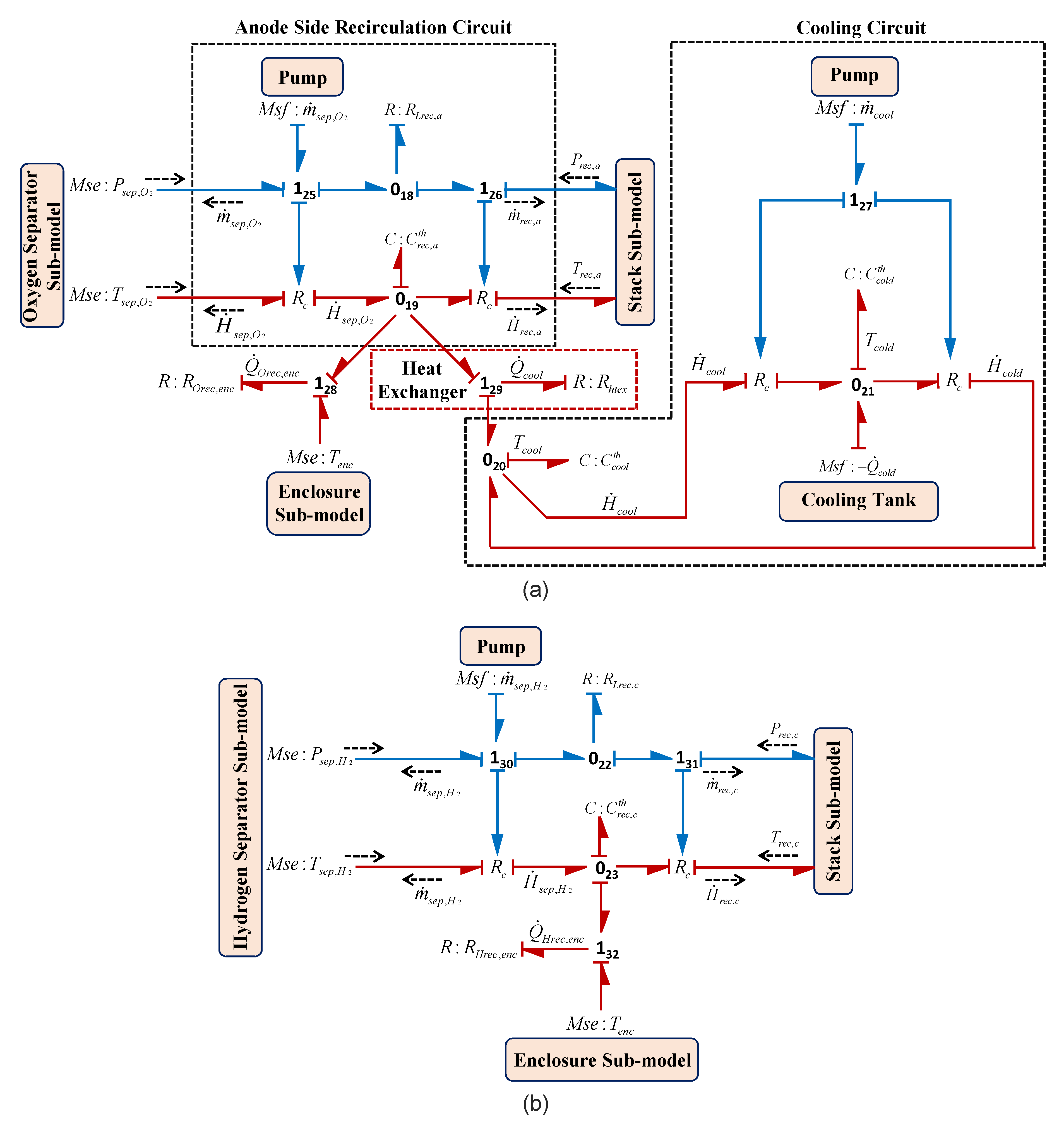
3.2.4. Cooling and Recirculation Circuits

The desired temperature of the stack is automatically maintained by the cooling and the recirculation system by getting the information of hydrogen and oxygen production along with the information of heat flow in this system. The recirculation system has its own process and instrumentation diagram which is used to feed the water at desired rate to the stack. In the current model the recirculation of water is done in each side of the cell, that is, anode and cathode side using a recirculating controlled pump. However at anode side, a heat exchanger along with its own cooling system is also incorporated which mainly maintains the stack temperature by controlling the input water temperature for the stack. The BG sub-model of this system for anode and cathode sides in capsule forms are shown in Figure 16a,b, respectively. The modelling of the cooling unit of the heat exchanger is also shown in Figure 16a. In the sub-model presented in Figure 16a, different pumps are model as the modulated source of flows M s f : m ˙ r e c , a and M s f : m ˙ c o o l , respectively, represent the anode side recirculating pump and the pump used for cooling of heat exchanger itself. The thermal capacity is modelled by the lump parameter C : C r e c , a t h . Thus, from the Figure 16a, using constitutive relation of C : C r e c , a t h and junction 0 19 , anode side recirculation temperature can be obtained as
T r e c , a = 1 C r e c , a t h H ˙ s e p , O 2 H ˙ r e c , a Q ˙ O r e c , e n c Q ˙ c o o l d t ,
where the enthalpy flows in the anode side recirculation system H ˙ s e p , O 2 and H ˙ r e c , a are calculated from the Equation (35). The heat dissipation, Q ˙ O r e c , e n c , due to temperature gradient between recirculation system and enclosure is modelled by BG generalized resistive element R : R O r e c , e n c and Q ˙ c o o l is the extracted rate of heat flow by the heat exchanger which is modelled by using resistive element R : R h t e x . In order to calculate the Q ˙ c o o l , the Number of Transfer Unit (NTU) technique is used for heat exchanger [51].
Likewise, for the sub-model of cooling unit of the heat exchanger in Figure 16a, using constitutive relations of C : C c o o l t h , C : C c o l d t h and junctions 0 20 , 0 21 temperatures T c o o l , T c o l d can be obtained as
T c o o l = 1 C c o o l t h H ˙ c o l d H ˙ c o o l + Q ˙ c o o l d t ,
T c o l d = 1 C c o l d t h H ˙ c o o l H ˙ c o l d Q ˙ c o l d d t ,
where T c o o l , T c o l d and C c o o l t h , C c o l d t h are the temperatures and thermal heat capacities of cooling system of heat exchanger and cooling tank for the coolant, respectively. In sub-model of cooling unit in Figure 16a, M s f : m ˙ c o o l represents the coolant mass flow which is used for the calculation of H ˙ c o o l and H ˙ c o l d using Equation (35) with temperatures T c o o l and T c o l d , respectively.
Likewise, using the sub-model of recirculation system in cathode side as shown in Figure 16b, using constitutive relation of C : C r e c , c t h and junction 0 23 , cathode side recirculation temperature can be obtained as
T r e c , c = 1 C r e c , c t h H ˙ s e p , H 2 H ˙ r e c , c Q ˙ H r e c , e n c d t ,
where the enthalpy flows in the cathode side recirculation system H ˙ s e p , H 2 and H ˙ r e c , c are calculated from the Equation (35). The lump parameter C : C r e c , c t h is used to model its thermal capacity towards the cathode side.

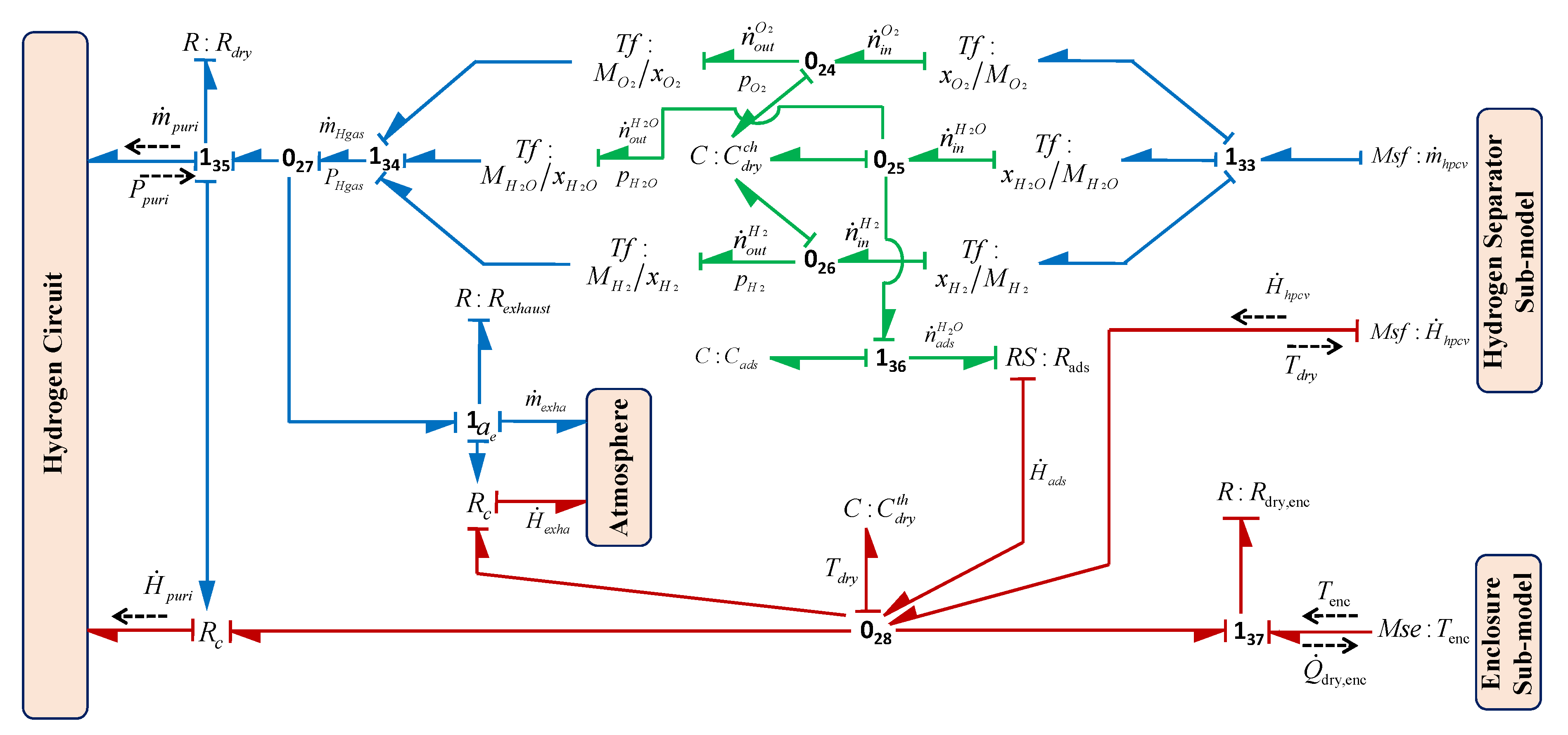
3.2.5. Hydrogen Purification Subsystem

This unit purifies the gas according to the preset hydrogen purity level required for the particular application. A dryer is used which removes the unwanted moisture from the gas by adsorbing the fraction of water content in it. The modelling of this unit requires the coupling of thermal, chemical and fluidic phenomena. The BG sub-model of the purification subsystem is shown in Figure 17. The lump parameters C : C d r y t h , R : R d r y , e n c , R : R d r y , R : R e x h a u s t , C : C d r y c h , C : C a d s c h and R S : R a d s are, respectively, used to model the thermal capacity, thermal resistance, internal pneumatic resistance, exhaust resistance, dryer chemical capacity, water adsorption capacity and the adsorption resistance of the unit. Here, element R S : R a d s is used to couple the chemical and thermal phenomena of the unit. According to Figure 17, using constitutive relation of C : C d r y t h and junction 0 28 , dryer temperature T d r y can be obtained as
T d r y = 1 C d r y t h H ˙ h p c v + H ˙ a d s H ˙ p u r i Q ˙ d r y , e n c a e × Q ˙ e x h a d t ,
where H ˙ h p c v is the enthalpy flow coming through hydrogen pressure control valve, H ˙ a d s = n ˙ a d s H 2 O × Δ H a d s is the enthalpy flow due to fraction of water adsorption with molar flow n ˙ a d s H 2 O in the reaction, H ˙ p u r i enthalpy flow out from the purification system toward hydrogen production, Q ˙ d r y , e n c is the rate of heat loss due to temperature gradient between dryer unit and system enclosure and H ˙ e x h a is the enthalpy flow when the exhaust valve is on ( a e = 1 ).
Likewise, according to Figure 17, using constitutive relations of C : C d r y , i t and junction 0 24 / 0 26 for partial pressures p d r y , i of oxygen and hydrogen gases, respectively, and C : C d r y , j c h and junction 0 25 for partial pressure p d r y , j of water vapour can be obtained as
p d r y , i = 1 C d r y , i c h m ˙ h p c v × x i M i m ˙ p u r i × x i M i d t
p d r y , j = 1 C d r y , j c h m ˙ h p c v × x j M j m ˙ p u r i × x j M j n ˙ a d s j d t ,
where m ˙ h p c v is the mass inflow coming through hydrogen pressure control valve, m ˙ p u r i mass outflow from the purification system towards hydrogen production, x i and x j are the respective mass fractions. The capacities C d r y , i c h and C d r y , j c h can be similarly obtained from Equation (36) for the different species. The total pressure P d r y of the dryer is the summation of partial pressure of the gases.

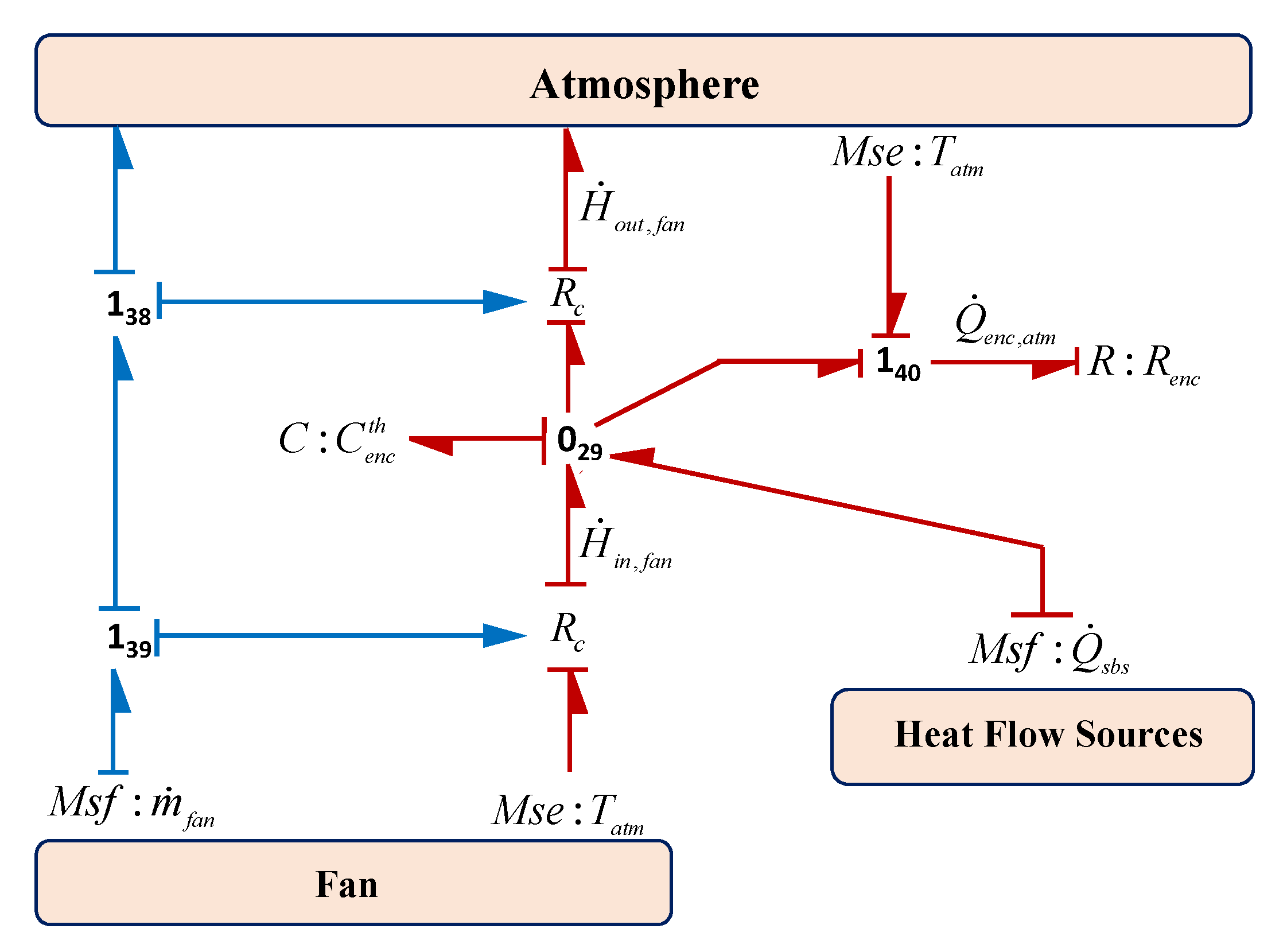
3.2.6. System Enclosure

The major subsystems of the electrolysis system are kept inside an enclosure which is designed according to the environmental requirements and the different functions of the subsystems. The enclosure temperature is maintained at desired temperature by designing the proper venting system and providing the fan/blower for its cooling. The BG sub-model of the system enclosure is shown in Figure 18. In this sub-model, the fan is modelled by the source of flow generalized BG element ( M S f : m ˙ f a n ) to represent the mass flow of air and the atmospheric temperature is modelled as the source of effort generalized BG element ( M S e : T a t m ). The thermal capacity and the thermal resistance are modelled by the lumped parameters using C : C e n c t h and R : R e n c . Thus, from Figure 18, using constitutive relation of C : C e n c t h and junction 0 29 , enclosure temperature T e n c can be obtained as
T e n c = 1 C e n c t h Q ˙ s b s + H ˙ i n , f a n H ˙ o u t , f a n Q ˙ e n c , a t m d t ,
where Q ˙ s b s is the summation of all the rate of heat losses from the different subsystems to the enclosure, H ˙ i n , f a n and H ˙ o u t , f a n are the rate of heat enthalpy in to the enclosure and out from it which depend on the specific heat ( C P , a i r ) and the mass flow of air ( m ˙ f a n ). Also, Q ˙ e n c , a t m is the rate of heat loss to the atmosphere.

3.3. Efficiency of the PEM Electrolysis System

For analyzing the performance of the electrolysis system, efficiency is also the one of the most important parameters whose definition mainly depends on the different operating conditions and the system designs. Here, the efficiency is defined in the two levels: (i) cell/stack level (ii) system level including the auxiliaries. Here, it is also assumed that the cell operating voltage is always greater than the thermal-neutral voltage. Also, operating temperature is below the boiling point of water and water supplied in the liquid form. The real output of the system is only the useful hydrogen produced. Oxygen is not considered as a real output of the system, however it is also produced along with hydrogen.

3.3.1. Efficiency of Cell/Stack

For the dissociation of water in electrolysis process, a fixed amount of energy is required, which is equal to the summation of Gibbs free energy, Δ G R , and energy due to entropy change, T Δ S R , and this summed energies is called the enthalpy, Δ H R , of the electrolysis reaction. Here Δ G R is the minimum amount of energy that must be supplied by the electrical input by assuming the rest of energy is thermally contributed by T Δ S R term. The change in enthalpy ( Δ H R ) and Gibbs free energy ( Δ G R ) can be obtained from the chemical kinetics of the reaction as 286 kJ/mol and 237 kJ/mol, respectively, at standard temperature and pressure conditions, that equivalently represented in the form of standard electrode potential as 1.23 V and thermo-neutral potential as 1.48 V, respectively [52]. In the calculation of standard electrode potential in reversible condition, it is assumed that all the thermal energy along with electrical energy are contributed in the electrolysis reaction based on Lower Heating Value (LHV) that does not include enthalpy of evaporation of water. However, in the calculation of thermo-neutral potential it is assumed that only electrical energy is contributed in the electrolysis reaction based on Higher Heating Value (HHV) that includes enthalpy of evaporation of water. Thus, the efficiency calculation of an electrolysis system is based on either the HHV or the LHV and it should be quoted while mentioning the efficiency of the system. Thus, the efficiency can be defined as the ratio of energy or power content of the hydrogen produced based on HHV or LHV and the input electrical energy or power to the system. Usually, HHV is preferred over LHV to calculate the efficiency of an electrolysis system supplied with liquid water, as the enthalpy of evaporation has to be provided by the process and it is represented as in Equation (49) [42].
ε c e l l H H V = H H V × η ˙ H 2 P e l e c = H H V × η ˙ H 2 E c e l l × I c e l l ,
where η ˙ H 2 is molar flow of hydrogen and P e l e c is electrical DC input power to the electrolysis cell.
Efficiency ( ε d i s s ) for water dissociation can also be defined as the ratio of energy requirement in reversible condition ( E n r e v ) to the energy requirement in irreversible condition ( E n i r r e v ).
ε d i s s = E n r e v E n i r r e v .
Thus, based on Equation (50), other important efficiencies such as: voltage efficiency and current or Faradaic efficiency are also defined. Voltage efficiency can be obtained as the ratio of thermal-neutral voltage to the actual cell voltage at any operating condition, assuming the cell is always operating at a voltage above the thermal-neutral voltage. Thus, voltage efficiency is given as
ε v o l t = ε d i s s = E n r e v E n i r r e v = n × F × E t n n × F × E c e l l = E t n E c e l l .
Voltage efficiency as defined in Equation (51) can be analytically represented in the form of any operating temperature T   <   393.15 K as [53,54]
ε v o l t = 1.485 1.49 × 10 4 T T 0 9.84 × 10 8 T T 0 2 E c e l l .
The voltage efficiency as presented in Equation (51) is valid with the assumption that the current supplied to the cell is fully converted into electro-chemical reaction of water dissociation. However, this is not the real situation in the cell operation due to the presence of some stray current in the cell and the unintended side reactions. Furthermore, gases permeation through PEM and successive recombination to water and leakage of gas leads to a loss of actual production of hydrogen. To consider this, the current or Faradaic efficiency ε c u r r is defined, which is the ratio of actual hydrogen produced ( η ˙ H 2 , a c t ) to the theoretically hydrogen produced ( η ˙ H 2 , t h ) based on Faraday’s law.
ε c u r r = η ˙ H 2 , a c t η ˙ H 2 , t h = η ˙ H 2 , a c t I / n F .
Thus, the overall cell efficiency can be obtained by multiplying voltage and current efficiency as
ε c e l l = ε v o l t × ε c u r r .

3.3.2. Efficiency of System Including the Auxiliaries

Electrolysis system includes the various other supporting subsystems and auxiliaries for the production of green hydrogen. Every auxiliaries and subsystems have their own efficiency which can be estimated or supplied by the manufacturer. It is assumed that an imaginary boundary is considered that includes the electrolysis cell and the supporting auxiliaries for defining the system efficiency. Here, solar and/or wind subsystems are excluded for defining the system efficiency. Thus, the efficiency of the complete system is ratio of the energy content of hydrogen produced and the total amount of energy consumed and it is given as
ε s y s t H H V = H H V × η ˙ H 2 P s y s t = H H V × η ˙ H 2 P e l e c / ε c o n v + P p u m p + P h t e x + P o t h e r ,
where P s y s t is the total amount of energy or power consumed in the considered system, P e l e c denotes electrical DC input power and ε c o n v denotes converter efficiency, P p u m p denotes pump input power, P h t e x denotes input power to heat exchanger and P o t h e r denotes input power to other auxiliaries. However, there is always confusion and misunderstanding which heating value, that is, LHV or HHV, should be used in efficiency calculation. To eliminate this confusion, efficiency can be represented in terms of power consumed by the electrolysis system, which represents the amount of electrical energy consumed by the system to produce one kilogram (kWh/kg of H 2 ) or one normal cubic meter (kWh/Nm 3 of H 2 ) of hydrogen. It is noted that the efficiency calculation is constant when the electrical power input is constant. But, due to use of intermittent and time varying input sources, the value of efficiency changes with time. Thus, this needs the instantaneous calculation of efficiency [55].

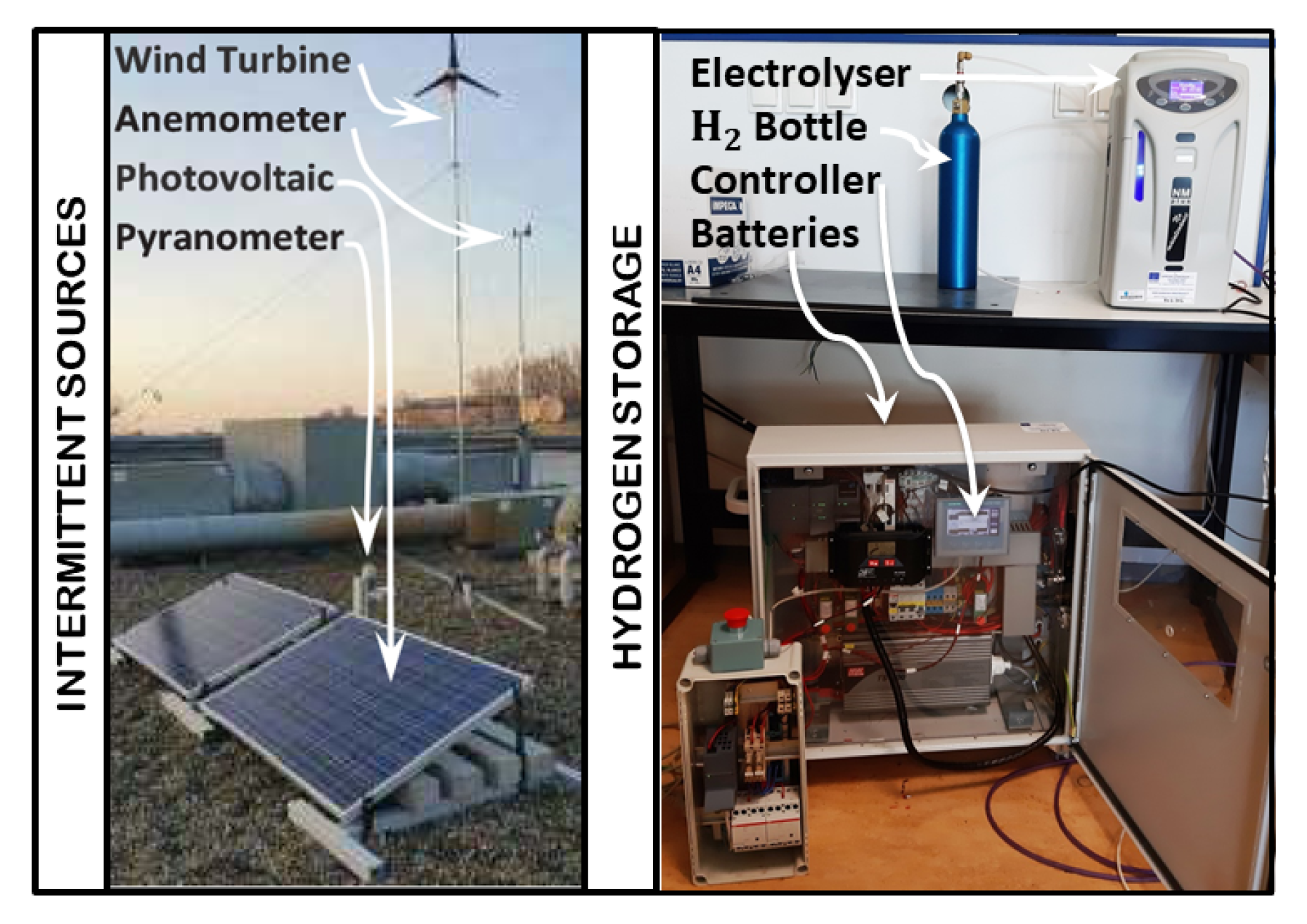
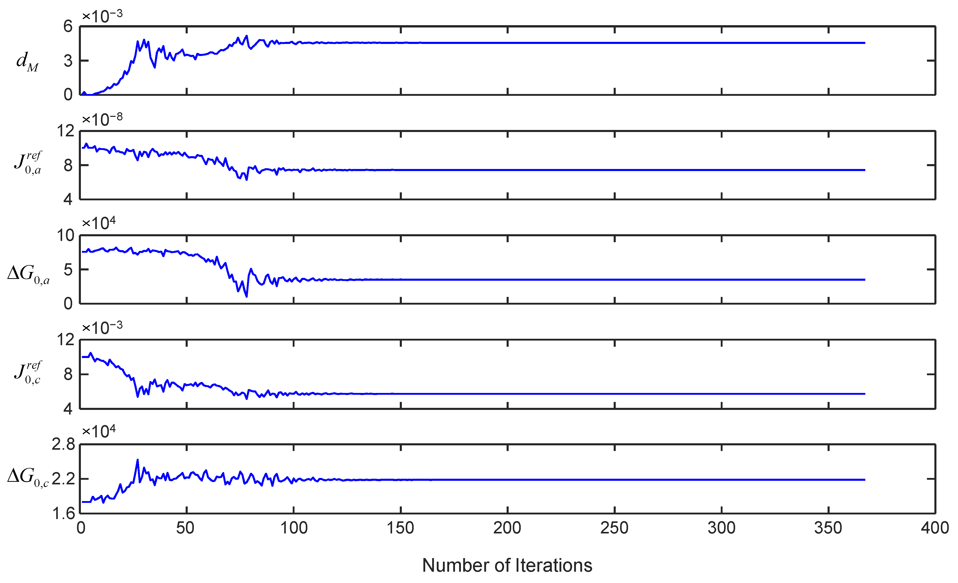
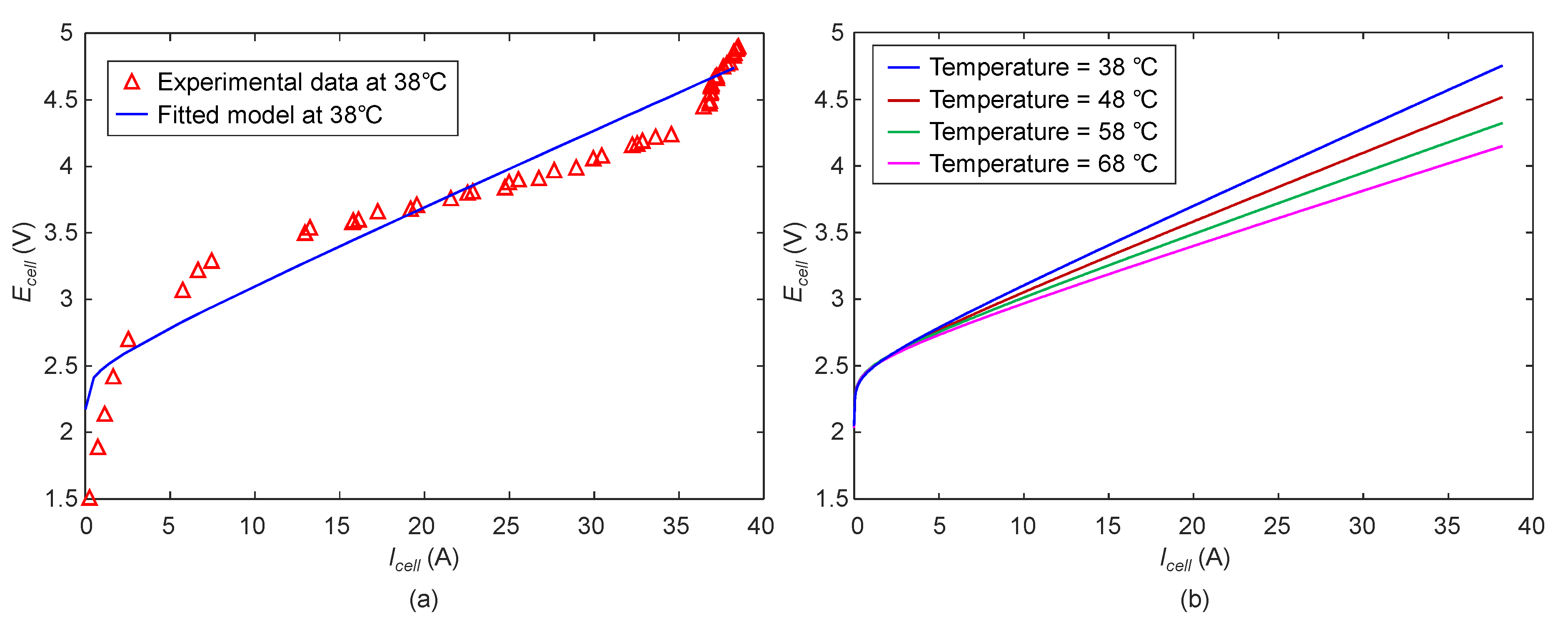
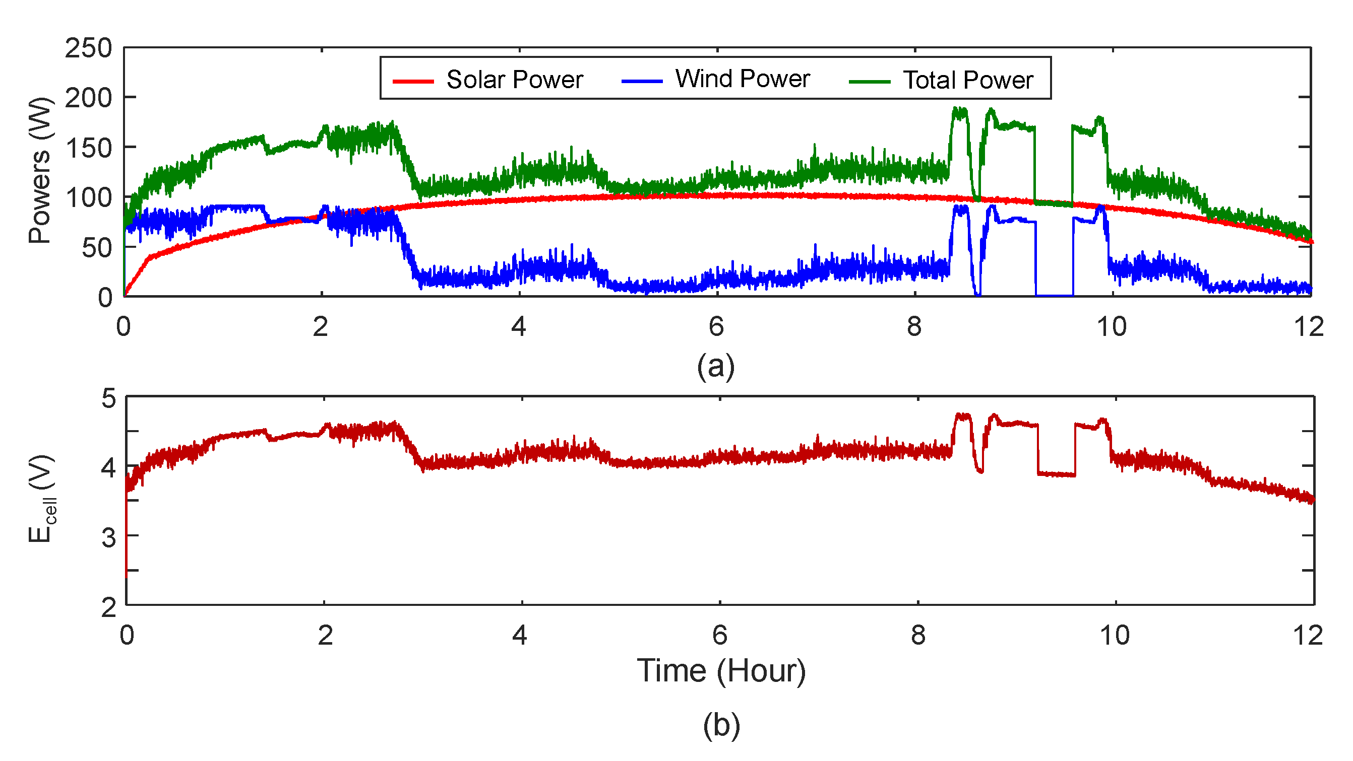
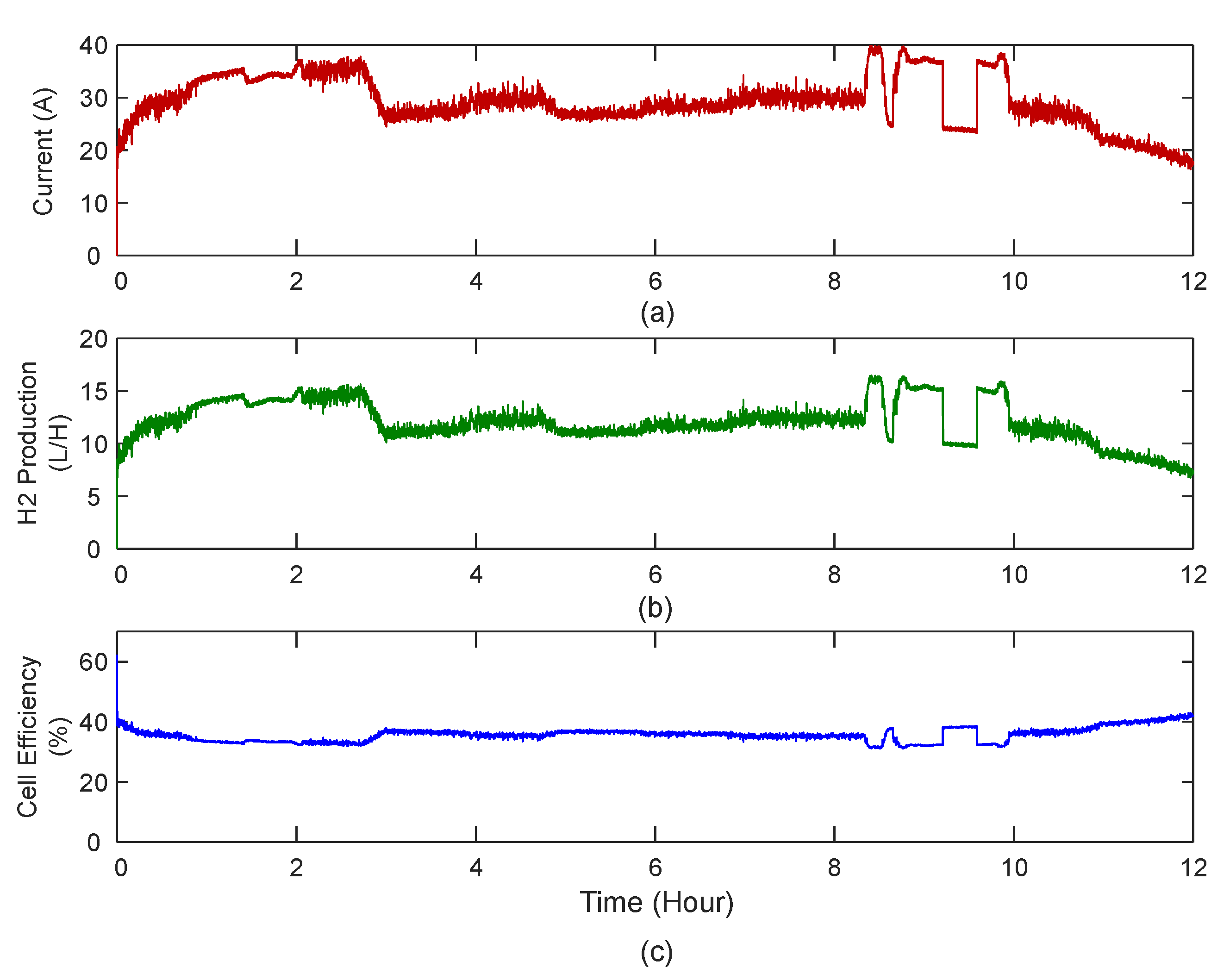
4. Experimental Validation and Results

The developed model is adapted for laboratory-scale electrolyser system running on a multi-source energy platform. For implementation viewpoint, Matlab-Simulink environment is used for simulation and sensor data acquisition through a programmable logic controller. The experimental platform of PEM electrolyser system running on intermittent sources is shown in Figure 19. The platform consists of two photo-voltaic panels (200 W power per panel), permanent magnet type wind turbine (350–400 W power) and two batteries (act as buffer with 55 Ah capacity per battery) running a commercial 300 W single cell PEM electrolyser. The electrolysis cell is fed with water at the anode side only and the produced hydrogen (pressure range 1.4–10.7 bar) is stored in the metal hydride canister (H 2 bottle) of 760 standard liter capacity.
In order to reduce the complexity, only the model of the electrolyser is considered and the intermittent sources are considered as an electrical source with signal noise (to represent intermittent nature).
For model validation, the key model parameters needs to be tuned with the experimental data. For example, the key parameters for the cell are identified using non-linear least square error optimization technique, which are shown in Figure 20. The bounds for the parameters values are taken from the literature for better estimation [8,24,42,54]. Other parameter values such as recirculation pump flow, height and cross-sectional area of hydrogen separator are taken based on the system specification provided by the manufacturer.
The polarisation (characteristic) curve from the actual measurements and the one estimated using the developed model is shown in Figure 21a. The mean absolute percentage error between simulation and experimental data is found to be 4.8% which is reasonable and well within the acceptable limit. Figure 21b shows the predicted characteristic curve at different temperatures. It can be seen that with the increase in the cell temperature the required cell voltage for electrolysis decreases. The predicted performance is in good agreement with the expected behaviour of the electrolyser found in the literature [18,24,42].
Figure 22a shows the contribution of different overvoltages in the overall cell voltage. It can be seen that with increase in the current the ohmic losses increases linearly. The contribution of the activation losses in the overall cell voltage remains almost constant. The losses due to mass transportation is negligible for small electrolysis cells and hence it is neglected. Figure 22b shows the variation of the cell efficiency with respect to the cell voltage.
The efficiency of the cell is constant till the cell voltage is less than thermo-neutral voltage. Once the cell voltage exceeds the thermo-neutral voltage, the efficiency decreases continuously. However, the efficiency at the system level can be calculated as discussed in Section 3.3.2, but, due to the limited number of the sensors placed in the experimental platform, the power consumed by different auxiliaries cannot be measured. Hence, the system level efficiency is not shown. Figure 22c shows the prediction of the temperature evolution of the cell from the thermal sub-model. The temperature starts rising from the ambient temperature and attains a constant value when the steady state of the operation is reached.
To predict the performance of the electrolyser powered by intermittent sources, a simulation of the electrolyser directly powered by the combination of solar and wind energy is performed. Figure 23a shows the total power fed to the cell by the converter and this figure also shows the individual contribution of each intermittent source. Figure 23b shows the input voltage to the electrolyser model with the objective of achieving high rate of hydrogen production.
The current drawn by the cell, the hydrogen production and the cell efficiency are shown in the Figure 24a–c respectively.
It can be seen that the efficiency of the cell is about 40%. This is due to the fact that the current electrolyser is designed to run at particular set point with the objective of delivering continuous hydrogen flow at higher rates. This is achieved by running the electrolyser at higher voltage (around 4 to 5 V) which results in reduced efficiency. In order to improve both efficiency and hydrogen production rate, the number of electrolysis cells should be increased.
In the current study, intermittent power is directly taken as an input for the model to predict the electrolyser’s performance. However, in real electrolysis system running on RES, the controller with buffer power source (battery) with operating mode management is always present [43]. This is important to maintain the constant input power to the cell in reference to the set point for stable operation and to avoid faster degradation of the cell membrane.

5. Conclusions

A generic multi-physics dynamical model of PEM electrolyser (including the auxiliaries) is developed using the BG approach. The developed model consists of sub-models (capsules) that can be easily modified to fit any PEM electrolyser. Because of the generic nature, it can be easily sized and scaled as per the requirement. The model incorporates the efficiency of stack and auxiliaries in order to estimate the performance of the electrolyser. Also, the system dynamics and the different thermal losses can be predicted which cannot be done in the real process. With the increase in current density, efficiency of the electrolyser decreases due to the reduction in the performance and corresponding heat dissipation. Final implementation and simulations are performed on MATLAB-Simulink. The validation of the model has been done statically against the experimental data from a single cell PEM electrolyser running on intermittent sources (solar and wind). The accuracy of the validation corresponds to the industrial requirements as the error is found to be 4.83%. However, the model is capable of capturing the effect of system dynamics with the parameters variation; but, due to the industrial constraints on the parameters identification, the model validation in different dynamic configurations is not performed.
The developed model is economical in nature. Due to the use of specific formalism (causal and structural properties of the BG), the developed model can not be used only for dynamic analysis but can also be used for control, diagnosis and prognosis studies. Therefore, this work is a foundation stone for the future work for developing model-based diagnosis and prognosis for PEM electrolysers. Since, the approach is modular and generic, the developed model can be extended to other types of electrolysers.

Author Contributions

Conceptualization, B.O.-B., J.-Y.D., M.B. (Mathieu Bressel), A.-L.G. and S.S.; methodology, S.S. and O.P.; software, M.B. (Mathieu Bressel), S.S. and O.P.; validation, S.S., O.P. and M.B. (Mahdi Boukerdja); formal analysis, S.S. and O.P.; resources, B.O.-B. and A.-L.G.; writing—original draft preparation, S.S., O.P. and M.B. (Mathieu Bressel); writing—review and editing, B.O.-B., J.-Y.D., M.B. (Mathieu Bressel) and A.-L.G.; supervision, B.O.-B., J.-Y.D. and M.B. (Mathieu Bressel); project administration, B.O.-B.; funding acquisition, B.O.-B. All authors have read and agreed to the published version of the manuscript.

Funding

This research work was funded under Interreg 2seas E2C project (subsidiary contract nr. 2S03-019).

Conflicts of Interest

The authors declare no conflict of interest.

Abbreviations

The following abbreviations are used in this manuscript:
AEMAnion Exchange Membrane
BGBond Graph
DCDirect Current
HHVHigher Heating Value
HSVHydrogen Separator Vessel
LHVLower Heating Value
MEAMembrane Electrode Assembly
NTUNumber of Transfer Unit
OSVOxygen Separator Vessel
PEMProton Exchange Membrane
RESRenewable Energy Sources
Nomenclature
α k Charge transfer or symmetry factor coefficients for k t h electrode
β Transformer coefficient of the converter
Δ G R Gibb’s free energy of water dissociation reaction, J·mol 1
Δ H R Enthalpy Change of water dissociation reaction, J·mol 1
Δ S R Entropy change of water dissociation reaction, J·mol 1 ·K 1
ξ ˙ Rate of reaction flow, mol·s 1
H ˙ Enthalpy rate, J·s 1
m ˙ i Mass flow rate of the i t h species, kg·s 1
n ˙ i Gas mass flow rate for i t h species, kg·s 1
Q ˙ Rate of heat flow, J·s 1
γ Hydration of the membrane
ν i Coefficient of stoichiometry for i t h species
ρ w Water density, kg·m 3
σ M Conductivity of the membrane, S·m 1
ε Efficiency
A M Cross-sectional area of the membrane, m 2
A s e p , i Cross-sectional area of the i t h separator, m 2
a H 2 O Chemical activity of water
C i Matter storage capacity of the i t h species ( i = H 2 , O 2 , H 2 O ), kg 2 ·J 1
C p Specific heat at constant pressure, J·kg 1 ·K 1
C c o l d t h Thermal capacitance of cooling tank, J·K 1
C c o o l t h Thermal capacitance of cooling circuit, J·K 1
C d r y , i c h Dryer’s chemical capacitance of the purification unit for the i t h species, mol·Pa 1
C d r y t h Dryer’s thermal capacitance of the purification unit, J·K 1
C e n c t h Thermal capacity of the enclosure, J·K 1
C H s e p , i c h Chemical capacitance of hydrogen separator for the i t h species, mol·Pa 1
C O s e p , i c h Chemical capacitance of oxygen separator for the i t h species, mol·Pa 1
C r e c , k t h Thermal capacitance of recirculation circuit (anode/cathode side), J·K 1
C s e p , H 2 f l t h Field capacitance element representing fluidic capacitance and thermal capacitance of hydrogen separator
C s e p , O 2 f l t h Field capacitance element representing fluidic capacitance and thermal capacitance of oxygen separator
C s t a c k Thermal capacitance of the stack, J·K 1
D i Parameter for diffusion, m 2 ·s 1
d M Ratio of length to the cross-sectional area of the membrane, m 1
E a c t , k Activation overvoltages for k t h electrode, V
E c e l l Cell voltage, V
E o h m Ohmic overvoltage, V
E r e v Reversible voltage, V
E r e v 0 Standard reversible cell voltage at STP, V
gAcceleration due to gravity, m·s 2
H i Henry’s Parameter, Pa·m 3 ·mol 1
I c e l l Cell current, A
JCurrent density, A·m 2
J 0 , k Standard current exchange density for k t h electrode, A·m 2
L M Length of the membrane, m
L s e p , i Water level in Separators (HSV and OSV), m
L s e p , i Water level of the i t h separator, m
M i Molar mass for i t h species, kg mol 1
n e o Electro-osmosis coefficient
PPressure, Pa
p i Partial pressure of i t h species, Pa
R c Coupling element for fluidic flow to thermal flow
R a c t , k Non linear activation resistance for k t h electrode
R a d s Coupling resistance of adsorbed water molar flow and the enthalpy flow towards dryer
R d i f f , i Diffusion resistance of the i t h species, Pa·s·kg 1
R d r y , e n c Thermal resistance between purification unit and enclosure, K·s·J 1
R d r y Internal pneumatic resistance of the dryer, Pa·s·kg 1
R e n c Thermal resistance between the enclosure and the atmosphere, K·s·J 1
R e x h a u s t Pneumatic resistance of the exhaust valve, Pa·s·kg 1
R H r e c , e n c Thermal resistance between hydrogen recirculation circuit and enclosure, K·s·J 1
R H s e p , e n c Thermal resistance between hydrogen separator and enclosure, K·s·J 1
R h t e x Thermal resistance of heat exchanger, K·s·J 1
R h y s t , k Internal fluidic resistance of the stack at th k t h electrode side, Pa·s·kg 1
R L r e c , k Hydraulic resistance representing leakage in recirculation circuit (anode/cathode side), Pa·s·kg 1
R o h m Total ohmic resistance of the cell, Ω
R O r e c , e n c Thermal resistance between oxygen recirculation circuit and enclosure, K·s·J 1
R O s e p , e n c Thermal resistance between oxygen separator and enclosure, K·s·J 1
R o t h e r s Ohmic resistance of the cell except membrane, Ω
R s e p , h c Pneumatic resistance between hydrogen separator and hydrogen circuit, Pa·s·kg 1
R s e p , o c Pneumatic resistance between oxygen separator and oxygen circuit, Pa·s·kg 1
R s e p v Hydraulic resistance of the separator valve, Pa·s·kg 1
R s t a c k Thermal resistance of the stack, K·s·J 1
R t a n k Hydraulic resistance between tank and oxygen Separator, Pa·s·kg 1
TTemperature, K
V H s e p , i Volume of the i t h species in HSV, m 3
V O s e p , i Volume of the i t h species in OSV, m 3
x i Mass fraction of the i t h species
μ i Chemical potential of the i t h species, J·kg 1
A i Chemical affinity of the i t h species, J·mol 1
C a d s c h Water adsorption capacity of the purification unit, mol·Pa 1
FFaraday’s constant, C·mol 1
RIdeal gas constant, J·mol 1 ·K 1

References

  1. Jain, I.P. Hydrogen the fuel for 21st century. Int. J. Hydrogen Energy 2009, 34, 7368–7378. [Google Scholar] [CrossRef]
  2. Olivier, P.; Bourasseau, C.; Ould-Bouamama, B. Low-temperature electrolysis system modelling: A review. Renew. Sustain. Energ. Rev. 2017, 78, 280–300. [Google Scholar] [CrossRef]
  3. David, M.; Ocampo-Martínez, C.; Sánchez-Peña, R. Advances in alkaline water electrolyzers: A review. J. Energy Storage 2019, 23, 392–403. [Google Scholar] [CrossRef] [Green Version]
  4. Vincent, I.; Bessarabov, D. Low cost hydrogen production by anion exchange membrane electrolysis: A review. Renew. Sustain. Energ. Rev. 2018, 81, 1690–1704. [Google Scholar] [CrossRef]
  5. Sood, S.; Ould-Bouamama, B.; Dieulot, J.Y.; Bressel, M.; Li, X.; Ullah, H.; Loh, A. Bond graph based multiphysic modelling of anion exchange membrane water electrolysis cell. In Proceedings of the 28th Mediterranean Conference on Control and Automation (MED), Saint-Raphaël, France, 15–18 September 2020; pp. 752–757. [Google Scholar] [CrossRef]
  6. Ipsakis, D.; Voutetakis, S.; Seferlis, P.; Stergiopoulos, F.; Elmasides, C. Power management strategies for a stand-alone power system using renewable energy sources and hydrogen storage. Int. J. Hydrogen Energy 2009, 34, 7081–7095. [Google Scholar] [CrossRef]
  7. Giddey, S.; Badwal, S.P.; Ju, H. Polymer electrolyte membrane technologies integrated with renewable energy for hydrogen production. In Current Trends and Future Developments on (Bio-) Membranes; Elsevier: Amsterdam, The Netherlands, 2019; pp. 235–259. [Google Scholar] [CrossRef]
  8. Carmo, M.; Fritz, D.L.; Mergel, J.; Stolten, D. A comprehensive review on PEM water electrolysis. Int. J. Hydrogen Energy 2013, 38, 4901–4934. [Google Scholar] [CrossRef]
  9. Wirkert, F.J.; Roth, J.; Jagalski, S.; Neuhaus, P.; Rost, U.; Brodmann, M. A modular design approach for PEM electrolyser systems with homogeneous operation conditions and highly efficient heat management. Int. J. Hydrogen Energy 2020, 45, 1226–1235. [Google Scholar] [CrossRef]
  10. Falcão, D.; Pinto, A.M.F.R. A review on PEM Electrolyzer Modelling: Guidelines for beginners. J. Clean Prod. 2020, 261, 121184:1–121184:10. [Google Scholar] [CrossRef]
  11. Saeed, W.; Warkozek, G. Modeling and analysis of renewable PEM fuel cell system. Energy Procedia 2015, 74, 87–101. [Google Scholar] [CrossRef] [Green Version]
  12. Xie, B.; Zhang, G.; Xuan, J.; Jiao, K. Three-dimensional multi-phase model of PEM fuel cell coupled with improved agglomerate sub-model of catalyst layer. Energy Convers. Manag. 2019, 199, 112051:1–112051:12. [Google Scholar] [CrossRef]
  13. Vuppala, R.K.; Chaedir, B.A.; Jiang, L.; Chen, L.; Aziz, M.; Sasmito, A.P. Optimization of Membrane Electrode Assembly of PEM Fuel Cell by Response Surface Method. Molecules 2019, 24, 3097. [Google Scholar] [CrossRef] [PubMed] [Green Version]
  14. Vijay, P.; Samantaray, A.K.; Mukherjee, A. A bond graph model-based evaluation of a control scheme to improve the dynamic performance of a solid oxide fuel cell. Mechatronics 2009, 19, 489–502. [Google Scholar] [CrossRef]
  15. Amiri, A.; Vijay, P.; Tadé, M.O.; Ahmed, K.; Ingram, G.D.; Pareek, V.; Utikar, R. Solid oxide fuel cell reactor analysis and optimisation through a novel multi-scale modelling strategy. Comput. Chem. Eng. 2015, 78, 10–23. [Google Scholar] [CrossRef] [Green Version]
  16. Hernández-Gómez, Á.; Ramirez, V.; Guilbert, D. Investigation of PEM electrolyzer modeling: Electrical domain, efficiency, and specific energy consumption. Int. J. Hydrogen Energy 2020, 45, 14625–14639. [Google Scholar] [CrossRef]
  17. Ruuskanen, V.; Koponen, J.; Huoman, K.; Kosonen, A.; Niemelä, M.; Ahola, J. PEM water electrolyzer model for a power-hardware-in-loop simulator. Int. J. Hydrogen Energy 2017, 42, 10775–10784. [Google Scholar] [CrossRef]
  18. Liso, V.; Savoia, G.; Araya, S.S.; Cinti, G.; Kær, S.K. Modelling and experimental analysis of a polymer electrolyte membrane water electrolysis cell at different operating temperatures. Energies 2018, 11, 3273. [Google Scholar] [CrossRef] [Green Version]
  19. Fragiacomo, P.; Genovese, M. Modeling and energy demand analysis of a scalable green hydrogen production system. Int. J. Hydrogen Energy 2019, 44, 30237–30255. [Google Scholar] [CrossRef]
  20. Hernández-Gómez, Á.; Ramirez, V.; Guilbert, D.; Saldivar, B. Cell voltage static-dynamic modeling of a PEM electrolyzer based on adaptive parameters: Development and experimental validation. Renew. Energy 2021, 163, 1508–1522. [Google Scholar] [CrossRef]
  21. Aubras, F.; Rhandi, M.; Deseure, J.; Kadjo, A.J.J.; Bessafi, M.; Majasan, J.; Grondin-Perez, B.; Druart, F.; Chabriat, J.P. Dimensionless approach of a polymer electrolyte membrane water electrolysis: Advanced analytical modelling. J. Power Sources 2021, 481, 228858:1–228858:10. [Google Scholar] [CrossRef]
  22. Zhou, T.; Francois, B.; el hadi Lebbal, M.; Lecoeuche, S. Modeling and control design of hydrogen production process by using a causal ordering graph for wind energy conversion system. In Proceedings of the IEEE International Symposium on Industrial Electronics, Vigo, Spain, 4–7 June 2007; pp. 3192–3197. [Google Scholar] [CrossRef]
  23. Agbli, K.; Péra, M.; Hissel, D.; Rallières, O.; Turpin, C.; Doumbia, I. Multiphysics simulation of a PEM electrolyser: Energetic Macroscopic Representation approach. Int. J. Hydrogen Energy 2011, 36, 1382–1398. [Google Scholar] [CrossRef]
  24. Olivier, P.; Bourasseau, C.; Ould-Bouamama, B. Dynamic and multiphysic PEM electrolysis system modelling: A bond graph approach. Int. J. Hydrogen Energy 2017, 42, 14872–14904. [Google Scholar] [CrossRef]
  25. Samantaray, A.K.; Ould-Bouamama, B. Model-Based Process Supervision: A Bond Graph Approach; Springer: London, UK, 2008. [Google Scholar] [CrossRef]
  26. Merzouki, R.; Samantaray, A.K.; Pathak, P.M.; Ould-Bouamama, B. Intelligent Mechatronic Systems: Modeling, Control and Diagnosis; Springer: London, UK, 2012. [Google Scholar] [CrossRef]
  27. Ould-Bouamama, B.; El Harabi, R.; Abdelkrim, M.N.; Gayed, M.K.B. Bond graphs for the diagnosis of chemical processes. Comput. Chem. Eng. 2012, 36, 301–324. [Google Scholar] [CrossRef]
  28. Prakash, O.; Samantaray, A.K.; Bhattacharyya, R. Model-based diagnosis of multiple faults in hybrid dynamical systems with dynamically updated parameters. IEEE Trans. Syst. Man Cybern. Syst. 2017, 49, 1053–1072. [Google Scholar] [CrossRef]
  29. Prakash, O.; Samantaray, A.K.; Bhattacharyya, R. Model-based multi-component adaptive prognosis for hybrid dynamical systems. Control Eng. Pract. 2018, 72, 1–18. [Google Scholar] [CrossRef]
  30. Prakash, O.; Samantaray, A.K.; Bhattacharyya, R. Adaptive Prognosis of Hybrid Dynamical System for Dynamic Degradation Patterns. IEEE Trans. Ind. Electron. 2019, 67, 5717–5728. [Google Scholar] [CrossRef]
  31. Paynter, H.M. Analysis and Design of Engineering Systems; The M.I.T. Press: Cambridge, MA, USA, 1961. [Google Scholar]
  32. Thoma, J.; Ould-Bouamama, B. Modelling and Simulation in Thermal and Chemical Engineering: A Bond Graph Approach; Springer-Verlag: Berlin/Heidelberg, Germany, 2000. [Google Scholar] [CrossRef]
  33. Ould-Bouamana, B.; Cassar, J.P. Integrated bond graph modelling in process engineering linked with economic systems. In Proceedings of the 14th European Simulation Multiconference on Simulation and Modelling: Enablers for a Better Quality of Life, Ghent, Belgium, 23–26 May 2000; pp. 340–347. [Google Scholar]
  34. Ould-Bouamama, B.; Abdalah, I.; Gehin, A.L. Bond graphs as mechatronic approach for supervision design of multisource renewable energy system. In Proceedings of the 5th International Conference on Mechanics and Mechatronics Research (ICMMR), Tokyo, Japan, 19–21 July 2018; pp. 012033:1–012033:5. [Google Scholar] [CrossRef] [Green Version]
  35. Samantaray, A.K.; Mukherjee, A. Users manual of SYMBOLS Shakti; High-Tech Consultants, STEP, Indian Institute of Technology: Kharagpur, India, 2006. [Google Scholar]
  36. Kleijn, C.; Groothuis, M.A.; Differ, H.G. 20-Sim 4.3 Reference Manual; Controllab Products: Hengelosestraat, The Netherlands, 2013. [Google Scholar]
  37. Ould-Bouamama, B.; Samantaray, A.K.; Medjaher, K.; Staroswiecki, M.; Dauphin-Tanguy, G. Model builder using functional and bond graph tools for FDI design. Control Eng. Pract. 2005, 13, 875–891. [Google Scholar] [CrossRef]
  38. Ould-Bouamama, B.; Staroswiecki, M.; Samantaray, A.K. Software for supervision system design in process engineering industry. IFAC Proc. Vol. 2006, 39, 646–650. [Google Scholar] [CrossRef]
  39. Ould-Bouamama, B. Bond graph approach as analysis tool in thermofluid model library conception. J. Frankl. Inst. 2003, 340, 1–23. [Google Scholar] [CrossRef]
  40. Görgün, H. Dynamic modelling of a proton exchange membrane (PEM) electrolyzer. Int. J. Hydrogen Energy 2006, 31, 29–38. [Google Scholar] [CrossRef]
  41. Abdin, Z.; Webb, C.; Gray, E.M. Modelling and simulation of a proton exchange membrane (PEM) electrolyser cell. Int. J. Hydrogen Energy 2015, 40, 13243–13257. [Google Scholar] [CrossRef]
  42. Bessarabov, D.; Wang, H.; Li, H.; Zhao, N. PEM Electrolysis for Hydrogen Production: Principles and Applications, 1st ed.; CRC Press: Boca Raton, FL, USA, 2016. [Google Scholar] [CrossRef]
  43. Abdallah, I.; Gehin, A.L.; Ould-Bouamama, B. Event driven Hybrid Bond Graph for Hybrid Renewable Energy Systems part I: Modelling and operating mode management. Int. J. Hydrogen Energy 2018, 43, 22088–22107. [Google Scholar] [CrossRef]
  44. Marangio, F.; Santarelli, M.; Cali, M. Theoretical model and experimental analysis of a high pressure PEM water electrolyser for hydrogen production. Int. J. Hydrogen Energy 2009, 34, 1143–1158. [Google Scholar] [CrossRef]
  45. García-Valverde, R.; Espinosa, N.; Urbina, A. Simple PEM water electrolyser model and experimental validation. Int. J. Hydrogen Energy 2012, 37, 1927–1938. [Google Scholar] [CrossRef]
  46. Kim, H.; Park, M.; Lee, K.S. One-dimensional dynamic modeling of a high-pressure water electrolysis system for hydrogen production. Int. J. Hydrogen Energy 2013, 38, 2596–2609. [Google Scholar] [CrossRef]
  47. Nafchi, F.M.; Afshari, E.; Baniasadi, E.; Javani, N. A parametric study of polymer membrane electrolyser performance, energy and exergy analyses. Int. J. Hydrogen Energy 2019, 44, 18662–18670. [Google Scholar] [CrossRef]
  48. Awasthi, A.; Scott, K.; Basu, S. Dynamic modeling and simulation of a proton exchange membrane electrolyzer for hydrogen production. Int. J. Hydrogen Energy 2011, 36, 14779–14786. [Google Scholar] [CrossRef]
  49. Grigoriev, S.; Porembskiy, V.; Korobtsev, S.; Fateev, V.; Auprêtre, F.; Millet, P. High-pressure PEM water electrolysis and corresponding safety issues. Int. J. Hydrogen Energy 2011, 36, 2721–2728. [Google Scholar] [CrossRef]
  50. Chandesris, M.; Médeau, V.; Guillet, N.; Chelghoum, S.; Thoby, D.; Fouda-Onana, F. Membrane degradation in PEM water electrolyzer: Numerical modeling and experimental evidence of the influence of temperature and current density. Int. J. Hydrogen Energy 2015, 40, 1353–1366. [Google Scholar] [CrossRef]
  51. Cengel, Y.; Ghajar, A. Heat and Mass Transfer: Fundamentals and Applications, 5th ed.; McGraw Hill Education: New Delhi, India, 2017. [Google Scholar]
  52. Scheepers, F.; Stähler, M.; Stähler, A.; Rauls, E.; Müller, M.; Carmo, M.; Lehnert, W. Improving the efficiency of PEM electrolyzers through membrane-specific pressure optimization. Energies 2020, 13, 612. [Google Scholar] [CrossRef] [Green Version]
  53. LeRoy, R.L.; Bowen, C.T.; LeRoy, D.J. The thermodynamics of aqueous water electrolysis. J. Electrochem. Soc. 1980, 127, 1954–1962. [Google Scholar] [CrossRef]
  54. Bessarabov, D.; Millet, P. PEM Water Electrolysis; Academic Press: Cambridge, MA, USA, 2017; Volume 1. [Google Scholar] [CrossRef]
  55. Bessarabov, D.; Millet, P. PEM Water Electrolysis; Academic Press: Cambridge, MA, USA, 2018; Volume 2. [Google Scholar] [CrossRef]
Figure 1. Schematics of PEM electrolyser cell.
Energies 13 06556 g001
Figure 2. (a) General schematic of a Proton Exchange Membrane (PEM) electrolyser and (b) Multi-physics phenomena in PEM electrolyser cell/stack (inspired by Reference [2]).
Energies 13 06556 g002
Figure 3. (a) Causal Bond Graph (BG) and (b) corresponding block diagram representation.
Energies 13 06556 g003
Figure 4. Representation of vector bond (a) with a small ring around the power bond, (b) with multi-bonds and (c) with separate power bond for different energy domains.
Energies 13 06556 g004
Figure 5. (a) Schematic diagram and (b) BG model of PEM electrolyser stack capsule.
Energies 13 06556 g005
Figure 6. Graphical user interface of the model builder.
Energies 13 06556 g006
Figure 7. (a) Invalid and (b) Valid connection of capsules.
Energies 13 06556 g007
Figure 8. The word BG model of the electrolysis system.
Energies 13 06556 g008
Figure 9. Electrochemical BG sub-model in capsule form.
Energies 13 06556 g009
Figure 10. The BG chemical-fluidic sub-model in capsule form.
Energies 13 06556 g010
Figure 11. The BG thermal sub-model in capsule form.
Energies 13 06556 g011
Figure 12. BG sub-model of fluidic and mass transfer phenomenon in capsule form.
Energies 13 06556 g012
Figure 13. The global model of the stack of the PEM electrolysis system.
Energies 13 06556 g013
Figure 14. BG sub-model of converter subsystem.
Energies 13 06556 g014
Figure 15. BG sub-models (a) hydrogen separator and (b) oxygen separator.
Energies 13 06556 g015
Figure 16. BG recirculation sub-models (a) anode side including cooling circuit and (b) cathode side.
Energies 13 06556 g016
Figure 17. BG sub-model purification subsystem in capsule form.
Energies 13 06556 g017
Figure 18. BG sub-model of system enclosure in capsule form.
Energies 13 06556 g018
Figure 19. Experimental platform of the PEM electrolyser running on intermittent sources.
Energies 13 06556 g019
Figure 20. Parameter estimation for the sub-model of the stack.
Energies 13 06556 g020
Figure 21. (a) Comparison and (b) simulation of polarisation curve.
Energies 13 06556 g021
Figure 22. (a) Contribution of overvoltages, (b) efficiency of electrolysis cell and (c) temperature evolution of cell.
Energies 13 06556 g022
Figure 23. (a) Powers consumed by the cell for 12 h run and (b) Input voltage for the cell running on intermittent sources.
Energies 13 06556 g023
Figure 24. (a) Current drawn by the cell during 12 h of operation, (b) hydrogen production and (c) corresponding cell efficiency for the cell.
Energies 13 06556 g024
Table 1. Flow and effort for various energy domains.
Energy DomainFlow (f)Effort (e)
ElectricalCurrent intensity (A)Voltage (V)
FluidicVolume flow rate (m 3 ·s 1 )Pressure (Pa)
Fluidic (Pseudo BG)Mass flow (kg·s 1 )Pressure (Pa)
ThermalEntropy flow (J·K 1 ·s 1 )Temperature (K)
Thermal (Pseudo BG)Thermal flow (J·s 1 )Temperature (K)
Chemical (Transformation)Molar flow (mol·s 1 )Chemical potential (J·mol 1 )
Chemical (Kinetic)Reaction flow rate (mol·s 1 )Chemical affinity (J·mol 1 )
Publisher’s Note: MDPI stays neutral with regard to jurisdictional claims in published maps and institutional affiliations.

