Nonlinear Steady-State Optimization of Large-Scale Gas Transmission Networks

Abstract

The major optimization problem of the gas transmission system is to determine how to operate the compressors in a network to deliver a given flow within the pressure bounds while using minimum compressor power (minimum fuel consumption or maximum network efficiency). Minimization of fuel usage is a major objective to control gas transmission costs. This is one of the problems that has received most of the attention from both practitioners and researchers because of its economic impact. The article describes the algorithm of steady-state optimization of a high-pressure gas network of any structure that minimizes the operating cost of compressors. The developed algorithm uses the “sequential quadratic programming (SQP)” method. The tests carried out on the real network segment confirmed the correctness of the developed algorithm and, at the same time, proved its computational efficiency. Computational results obtained with the SQP method demonstrate the viability of this approach.

1. Introduction

Gas transmission systems have been used for many years to transport natural gas across long distances using compressor stations. The compressors consume a part of the transported gas, which results in an important fuel consumption cost. Optimization of the running cost of compressor stations plays an important role in the operating costs of the stations. The difficulties of such optimization problems are caused by the nonlinearity of the problem—the nonlinear objective function and the set of constraints imposed on feasible operating conditions in the compressors, along with the constraints in the pipelines, constitute a very complex system of nonlinear constraints. The growing complexity of gas transmission systems is accompanied by increasing opportunities for more efficient management.

Gas compressor stations form a major part of the operational plant in every transmission system. Their function is to restore gas pressure reduction caused by frictional pressure losses. The compressors are driven mostly by gas turbines that use natural gas as fuel, taken directly from the transmission pipelines.

The compressor unit comprises three main components: a gas generator, a power turbine and a centrifugal gas compressor.

The maximum shaft power of the units ranges from 5.5 MW to more than 20 MW, while the associated fuel consumptions are equivalent to 8600 to 19,000 pounds of fuel cost per day.

The value of the compressor fuel used in the UK exceeds 60 million pounds per annum [1]. According to [2], the operating cost of running the compressor stations represents between 25% and 50% of the total company’s operating budget.

The operating costs of the gas transmission system are high.

The major optimization problem is that of determining how to operate the compressors in a network to deliver a given flow while using minimum compressor power (minimum fuel consumption or maximum network efficiency).

Minimization of fuel usage is a major objective to control gas transmission costs.

The paper is structured as follows: Section 2 provides a brief literature review for steady-state optimization of gas networks. A steady-state optimization process of gas networks is explained in Section 3. In Section 4, the steady-state optimization problem of gas networks is formulated. Objective function and constraints are described in detail, while in Section 5, the problem solution using the sequential quadratic programming method is characterized. Section 6 contains a case study. The results of the case study are discussed in Section 7. The last section presents the conclusions of this paper.

2. Literature Review

An overview of different optimization techniques used for managing gas transport in pipeline networks can be found in a review paper [3]. Examples of the optimization problems under transient conditions include a line-packing problem and compressor station fuel cost minimization problems, as described in [4] and [5]. The compressor station fuel cost minimization problems are based upon hierarchical control and decomposition or mathematical programming approaches. The studies on hierarchical control include [6,7,8,9,10].

When modeling systems, however, it is sometimes convenient to make a simplifying assumption that the flow is steady. Under many conditions, this assumption produces adequate engineering results. For many years, control methods for these systems have been developed in various research centers around the world, aimed at reducing operating costs. For this purpose, various algorithms for linear, nonlinear, mixed, or dynamic optimization are used, depending on the assumptions made by the authors and the degree of simplification of the problem.

The mathematical programming approaches to optimization of gas networks of an arbitrary structure under steady-state conditions include the linearization of the objective function and constraints, resulting in a solution of linear programming problem in [11], quadratic programming problem as a consequence of linear approximations of the nonlinear flow–pressure relations in pipes in [12], and gradient-search-based methods in [13]. Mathematical programming approaches are used to formulate and solve nonlinear programming problems in [14,15], mixed-integer linear programming problems based on piecewise linearization in [16,17], or a combination of the linear and nonlinear formulations in [18].

The fuel cost minimization of steady-state gas pipeline networks can also be tackled with dynamic programming methods, as in [1] and [19]. Gas flow in the pipeline networks governed by the isothermal Euler equations and new modeling of compressors in gas networks are considered in [20] for optimization of gas networks.

A modified algorithm of evolution strategies that can solve a large class of steady-state optimization problems is described in [21]. A pipeline operation optimization model with minimum energy consumption as the objective function was established on the basis of the dynamic programming method in [22].

An efficient minimization scheme of gas compression costs under dynamic conditions where deliveries to customers are described by time-dependent mass flow is given in [23].

It needs to be stressed that further detailed compressor station submodels are established for the solution of fuel cost minimization problems in gas network optimization problems. A local optimization procedure of the compressor station involving minimization of the compressor driver’s fuel consumption based on mixed-integer nonlinear programming was formulated in [7], while in [24] an algorithm of an automatic search for the optimal values of the operating parameters of the compressor station was proposed. The algorithm automatically searches the number of simultaneously operating compressors and their capacity distribution. The implementation of the above local optimization procedure and an algorithm for optimal control of a compressor station installed in a simple transmission system was recently discussed in [25].

In [26], the optimization of the fuel consumption of the compressors through manipulation of the effective parameters of the turbines and the air coolers within a gas compressor station unit in the operation phase by use of a genetic algorithm is described. Local optimization of the gas compressor station is described in [27]. The pipe flow is treated as a nonisothermal unsteady one-dimensional compressible flow. This is accomplished by treating the compressibility factor as a function of pressure and temperature and the friction factor as a function of Reynolds number. The solution method is the fully implicit finite difference method, which provides solution stability, even for relatively large time steps.

The literature analysis shows that there has been and continues to be a significant effort focused on the optimization of natural gas transmission networks. Most of the discussed algorithms have solved the problems with different degrees of simplification concerning objective function and constraints (linearization, piecewise linearization, or combination of the linear and nonlinear formulations).

Compared to the above-discussed algorithms, the optimization algorithm discussed below solves the real problem, i.e., a nonlinear objective function with linear and nonlinear constraints, any structure of the network (with or without loops), and any number of pipes and nonpipe elements. At the same time, a very effective method (SQP) for nonlinearly constrained optimization problems was used. Verification of the algorithm using two nontrivial real gas networks confirms the correctness of the developed algorithm.

3. Steady-State Optimization

Depending on the character of gas flow in the system, we distinguish steady and unsteady states. The steady state in a gas network is described by the systems of algebraic nonlinear equations, and the unsteady state is described by partial differential equations.

It should be remembered that, apart from the minor exceptions resulting from the large storage capacity of gas pipelines, high pressure, and small changes in the network load, the gas transmission system is a transient state of gas flow. This means that, instead of nonlinear algebraic equations describing a steady gas flow, systems of parabolic or hyperbolic partial differential equations should be used depending on the nature and variability of the load over time. The use of such a mathematical model significantly complicates the optimization algorithm. In practice, static optimization algorithms are used either in the absence of an appropriate amount of data allowing for full dynamic optimization or as an algorithm whose task is to determine the correct starting point for the parent (dynamic) algorithm. This is a complete analogy with a simulation where the static simulator, especially for high-pressure networks with a complex structure and a large number of pipes, acts as a tool for determining the correct starting points for a dynamic simulator. In the case of an incomplete dataset, the static optimizer uses averaged load values over a specified period of time, and in the case of a full dataset, static optimization is performed for pressure and load values for t = 0 (t—time). In both cases, the use of the static optimization algorithm brings very good results. The optimization results obtained for the averaged values are important information for the compressor station operators, and the values obtained for the complete data set allow for a much more effective use of dynamic optimization.

In steady-state problems, since loads and supplies are not functions of time, an algorithm for optimization determines the structure of the network (i.e., the number of sources, compressors, valves, and regulators called units, which must be on). In addition, the algorithm must determine the optimal parameters of the operation, namely nodal pressures and flows through branches (pipes). For these reasons, the problem of optimization is formulated as a mixed-integer linear programming problem. Alternatively, assuming that the structure is known, an algorithm for steady-state optimization of large gas networks is treated as a nonlinear problem with nonlinear constraints. This case is analyzed in the paper.

4. Optimization Problem—Formulation

The amount of energy input to the gas by the compressors is dependent upon the pressure of the gas and the flow rate. The head developed by the compressors is defined as the amount of energy supplied to the gas per unit mass of gas. By multiplying the mass flow rate of gas by the compressor head, we can calculate the total energy supplied to the gas. Dividing this by compressor efficiency, we will obtain the horsepower that represents the energy per unit time required to compress the gas. The equation for horsepower can be expressed as follows [28]:

$$HP=\frac{M · H}{\eta }$$

(1)

where:

M—mass flow rate of gas (kg/s);

HP—compressor horsepower (W);

H—compressor head (J/kg);

$\eta$—compressor efficiency, decimal value.

To calculate polytropic head we use the following equation [28]:

$$H=\frac{Z R T}{\left(n-1\right)\eta }\left[{\left(\frac{p_d}{p_s}\right)}^{\left(n-1\right)/n}-1\right]\hspace{1em}\hspace{1em}\left[W\right]$$

(2)

where:

Z—gas compressibility factor;

R—the individual gas constant (J/kgK);

T—absolute temperature (K);

n—isentropic exponent;

$\mathsf{\eta }$—adiabatic efficiency;

${\mathrm{p}}_{\mathrm{d}}$—discharge pressure;

${\mathrm{p}}_{\mathrm{s}}$—suction pressure.

Finally, Equation (1) takes the following form:

$$HP=\frac{n p_s Q_s}{\eta 3600 \left(n-1\right)T_s}\left[{\left(\frac{p_d}{p_s}\right)}^{\left(n-1\right)/n}-1\right]\hspace{1em}\hspace{1em}\left[ W\right]$$

(3)

where:

ps—pressure at standard conditions (Pa);

Qs—volumetric gas flow through the i-th compressor station at standard conditions (m³/h);

Ts—temperature at standard conditions K.

The goal of steady-state optimization of the transmission gas network is to minimize fuel consumption (which is a linear function of horsepower). The objective function minimized in the optimization process has the following form:

$$HP={{\displaystyle \sum }}_{i=1}^{k}H{P}_i={{\displaystyle \sum }}_{i=1}^k\frac{n p_s Q_s}{\eta 3600 \left(n-1\right)T_s}\left[{\left(\frac{p_{d,i}}{p_{s,i}}\right)}^{\left(n-1\right)/n}-1\right]\hspace{1em}\hspace{1em}\left[W\right]$$

(4)

HP_i—power consumption for the i-th compressor station (W);

p_d,i—discharge pressure for the i-th compressor station (Pa);

p_s,i—suction pressure in for the i-th compressor station (Pa);

k—number of switch-on compressor stations in the system (–).

The gas network is modeled as a network consisting of two kinds of branches: pipe branches, for which there is a pressure loss equation, and nonpipe elements (valve, compressor, regulator, compressors station, source), which do not have a pressure loss equation. Nonpipe elements are subject to the constraints on functions of flow as well as inlet and outlet pressures. Mass balance equation applies to all nodes. In our model, temperature distribution is assumed known. The other components of the model are input flow or pressure from “source” nodes, which are constant, and output flow “demand”, which is known.

4.1. Constraints

For the high-pressure gas networks, operating above 7.0 bar gauge, the Panhandle A equation is used. The Panhandle A equation was derived from the fundamental energy equation for compressible flow [29,30]. For each pipe k (having node l(k) at its left and node r(k) at its right), the pressure drop equation has the following form:

$$p_{l\left(k\right)}^2-p_{r\left(k\right)}^2=K{Q}^{1,854}$$

(5)

where:

p—pressure;

Q—flow through pipe.

$$\mathrm{K}=18,43\frac{\mathrm{L}}{{\mathrm{E}}^2{\mathrm{D}}^{4,854}}$$

(6)

where:

L—pipe length;

D—pipe diameter;

E—pipe efficiency stated as a constant (~0.9).

For the whole of the network, the equality constraints are the following [31]:

$$\mathbf{A}\cdot \mathbf{Q}-\mathbf{K}\cdot \mathbf{F}-\mathbf{L}=\mathbf{0} (\mathbf{Kirchoff}‘\mathbf{s} \mathbf{first} \mathbf{law})$$

(7)

$$\mathbf{\Delta }\mathbf{P}+{\mathbf{A}}^{\mathbf{T}}\mathbf{\cdot }\mathbf{P}=\mathbf{0} (\mathbf{Kirchoff}‘\mathrm{s} \mathbf{second} \mathbf{law})$$

(8)

$$\mathbf{\Delta }\mathbf{P}={\mathrm{K}}_{\mathbf{f}}^{\mathbf{T}}\mathbf{\cdot }\mathbf{Q} (\mathbf{flow} \mathbf{equation})$$

(9)

where:

A—the nodal–branch incidence matrix (dim A = n × m);

n—the number of nodes;

m—the number of branches;

P—the vector of squared nodal pressures (dim P = n × 1);

K—the unit–nodal incidence matrix (dim K = n × r);

r—the number of units;

F—the vector of flows through units, (dim F = r × 1);

L—the vector of loads;

ΔP—the vector of squared drop pressures (dim ΔP = m × 1);

K_f—the vector of pipe constants (dim K_f = m × 1);

Q—the vector of flows through pipes (dim Q = m × 1).

For the given gas flows at every supply and delivery point in the networks, suction and discharge pressures should be determined at every compressor (consistent with set limits) so that fuel consumption is minimized.

It is always convenient, whenever possible, to reduce the amount of computer storage. In the above equations, matrices A, K and A^T have a large number of zero elements, thus making their full representation very inefficient. This could be reduced by using sparse matrix techniques. This method only uses the nonzero elements of a matrix. Let us use an example to illustrate the necessity of these methods. Taking the degree (the number of pipes incident to a node) as an average of 3 (the number of pipes incident to a node is by construction limited to 5), we calculate the percentage R of nonzero elements of an [n × m] matrix. The number of nonzero elements is then 3 times

$${\mathit{R}}_{\mathit{m}}=\frac{\mathbf{3}\mathit{n}}{\mathit{m}\mathit{n}}\mathbf{100}\%=\frac{\mathbf{3}}{\mathit{m}}\mathbf{100}\%$$

(10)

Thus, R₁₀ = 30%, R₁₀₀ = 3%, and R₁₀₀₀= 0.3%, in [23]. It can be seen that if m increases by 10, the percentage decreases by the same amount. For large gas networks, matrix A can be 1000 × 900 in dimension; therefore, the sparse matrix technique is very convenient.

4.2. Operational Constraints

The gas transmission system contains three types of controllable units, referred to as “nonpipe elements”. Upper and lower bounds are placed on all the nonpipe element flows and inlet and outlet pressures. These apply only when the nonpipe element is switched on.

In addition, bounds may be placed on any pressure in the network (including outlets and inlets). Sources and regulators are modeled using linear constraints, which are bounds on the pressure and flow. Compressors have both linear and nonlinear constraints.

4.3. Compressors

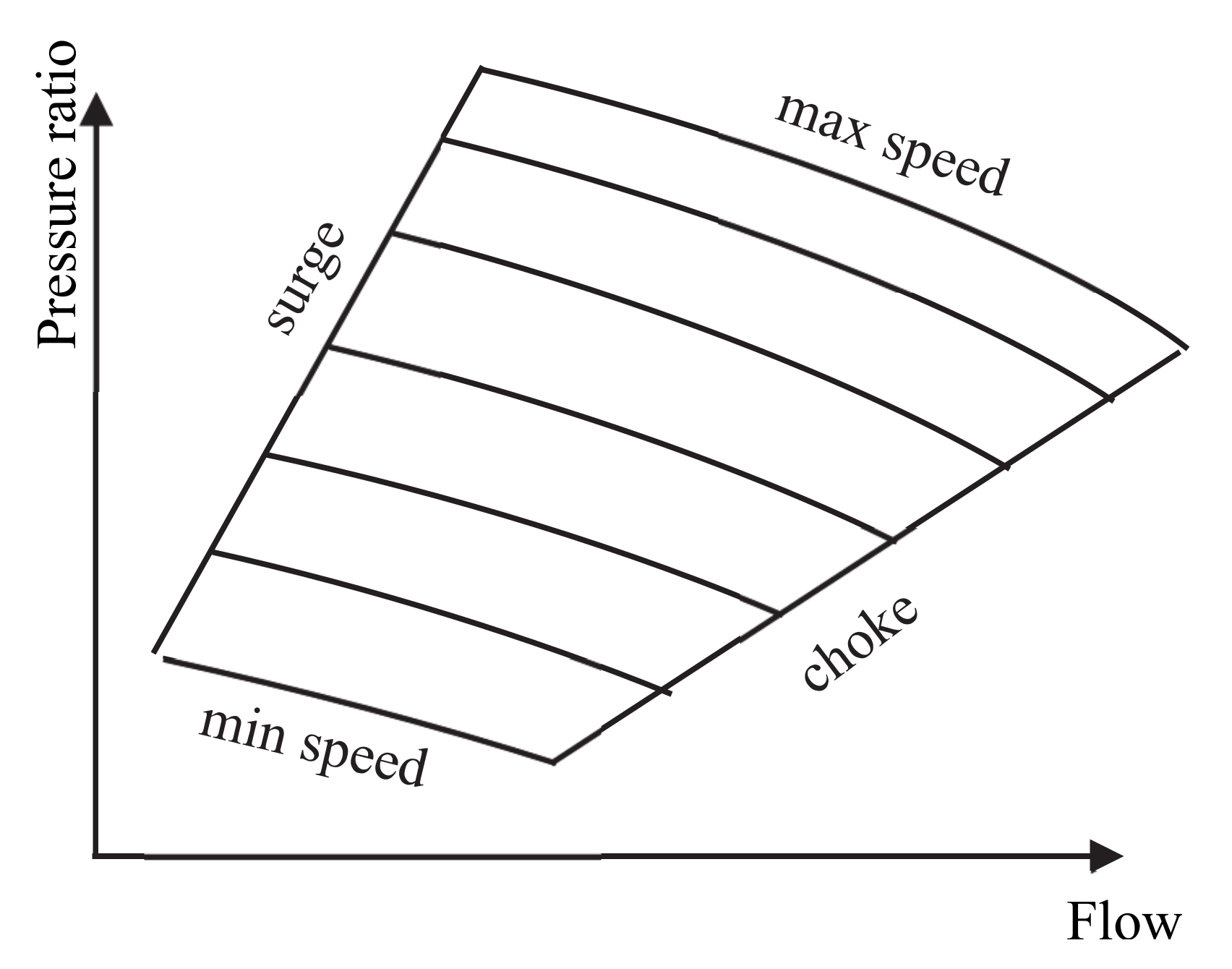
The centrifugal compressors used on the transmission system have particular characteristics. The operating regime can be expressed by what is known as an “envelope” (Figure 1). If the increase in pressure produced by a machine is plotted graphically against the flow, four limits, which enclose an area in which the compressor can properly run, emerge. The limits are defined as:

• “Surge”: This is the point at which flow through the compressor becomes so low that a reversal of flow can occur, which can be damaging to the compressor by causing high stress in the bearings or in the impeller. If all the points of minimum flow and corresponding pressure ratio are plotted, we get the surge line. This is the line at the left of the envelope.
• “Choke”: At the opposite end of the diagram, a compressor can reach choke. When the pressure ratio is low, there comes a point at which no further increase in flow through the compressor is possible.
• “Maximum and minimum speed”: Obviously, a compressor can run up to some given maximum speed consistent with machine safety; equally, there is a minimum speed line.

These four limits define the boundaries of the “envelope” of any compressor or combination of compressors. In the algorithm that is presented, constraints caused by the boundaries of the “envelope” were replaced with maximum compressor power (compression ratio and flow through compressor).

The surge line is formulated by the inequality [32,33]:

$${\mathrm{a}}_1\cdot {\mathrm{Q}}^2-{\mathrm{b}}_1\cdot \mathrm{Q}+1\ge \frac{{\mathrm{p}}_{\mathrm{d}}}{{\mathrm{p}}_{\mathrm{s}}}$$

(11)

where Q is the flow through the compressor (m³/h), a₁ and b₁ are specified coefficients, and choke line is formulated by the inequality [32,33]:

$${\mathrm{a}}_2\cdot {\mathrm{Q}}^2+{\mathrm{b}}_2\cdot \mathrm{Q}+1\le \frac{{\mathrm{p}}_{\mathrm{d}}}{{\mathrm{p}}_{\mathrm{s}}}$$

(12)

Surge line for the analyzed transmission system compressors is formulated by the inequality:

$$0.8355Q^2-0.05961Q+1\ge \frac{p_d}{p_s}$$

(13)

Choke line for the analyzed transmission system compressors is formulated by the inequality:

$$0.041879Q^2+0.021892Q+1\le \frac{p_d}{p_s}$$

(14)

Since all the compressors do not usually have the same characteristics, problems may occur when different types of compressors are running together. For instance, in a series arrangement, the maximum flow limit through one of the compressors may be lower than for the rest of the compressors, which imposes a flow limit on those compressors with a higher flow constraint. This is stated by the inequality:

$$Q_{max}\ge Q$$

(15)

where:

Q_max—maximum compressor flow;

Q—compressor inlet flow.

For the parallel arrangement, all the pressure ratios have to be equal. Therefore, the compressor with the lowest pressure ratio imposes a limit on the rest of the compressors with a higher pressure ratio. This is stated by the inequality:

$${\mathrm{CR}}_{\max }\ge \frac{p_d}{p_s}$$

(16)

where:

CR_max—maximum compressor ratio.

By construction, compressors have a maximum and a minimum speed limit. Operating beyond this upper limit may result in a damaged compressor. While operating below the lower limit, an unacceptable efficiency occurs. For the analyzed transmission system compressors, these constraints are formulated by the following inequality:

$$\mathit{R}\mathit{P}\mathit{M}\mathit{A}\mathit{X}\ge -\mathbf{1.6564}+\mathbf{2.02521}\mathit{Q}+\mathbf{9.1521}\frac{{\mathit{p}}_{\mathit{d}}}{{\mathit{p}}_{\mathit{s}}}-\mathbf{2.3541}{\left(\frac{{\mathit{p}}_{\mathit{d}}}{{\mathit{p}}_{\mathit{s}}}\right)}^{\mathbf{2}}-\mathbf{1.8946}\left(\frac{{\mathit{p}}_{\mathit{d}}}{{\mathit{p}}_{\mathit{s}}}\right)\mathit{Q}\ge \mathit{R}\mathit{P}\mathit{M}\mathit{I}\mathit{N}$$

(17)

where:

RPMAX—maximum speed (R.P.M.);

RPMIN—minimum speed (R.P.M.).

Finally, compressors have a maximum power that should not be exceeded. Developing more power than indicated by the limit may destroy the compressor. The power required by the prime mover is stated by the following inequality (1):

$$HP\le H{P}_{max}$$

(18)

4.4. Regulators

Flow through regulators is always unidirectional, which is stated by:

p_i > p_o

(19)

where:

p_i—inlet nodal pressure;

p_o—outlet nodal pressure.

There is an equation that relates inlet–outlet pressure difference to flow. If, for instance, for a particular regulator, the maximum drop pressure characteristic is known, the maximum permissible flow can be obtained through this equation, and vice versa. In our problem, we do not use that equation. Instead, we use the maximum flow obtained from that equation. The flow inequality constraint is:

$$Q_{max}\ge Q$$

(20)

where:

Q_max—maximum flow through regulator;

Q—actual flow through regulator.

Finally, the outlet pressure remains constant for any flow rate. This is stated by:

p_o = constant

(21)

4.5. Valves

There are several types of valves; however, for our purposes, only the isolating valves are of interest. These are used to interrupt the flow and to shut off sections of the network. In our problem, valves are represented by inequalities. The first one states that pressure difference is always greater upstream, that is:

p_i > p_o

(22)

where:

p_i—inlet pressure;

p_o—outlet pressure.

There is an equation for valves that relates their flow within the pressure difference throughout the valve. Since the maximum flow through the valve is given by the constructors, we can obtain the maximum pressure difference from the valve equation. Thus, we only need to define one constraint. In our problem, we have chosen the following flow inequality:

$$Q_{max}\ge Q$$

(23)

where:

Q_max—maximum flow through the valve;

Q—actual flow through the valve.

5. Problem Solution

The above problem has been formulated as nonlinear, with linear and nonlinear constraints in the following form:

$$\mathit{min}f\left(x\right)=\mathit{min}HP={{\displaystyle \sum }}_{i=1}^{k}H{P}_i={{\displaystyle \sum }}_{i=1}^k\frac{n p_s Q_s}{\eta 3600 \left(n-1\right)T_s}\left[{\left(\frac{p_{d,i}}{p_{s,i}}\right)}^{\left(n-1\right)/n}-1\right]\hspace{1em}\left[W\right]$$

(24)

subject to equality and inequality constraints

$$\left\{\begin{array}{c}ci\left(\mathit{x}\right)=0, i\in E\\ h_i\left(\mathit{x}\right)\ge 0, i\in I\end{array}\right.$$

(25)

where:

x^T = [p_d1,…, p_dk]—vector of discharge pressure;

E and I are finite index sets of equality and inequality constraints, respectively;

Function f(x) is continuous and differentiable.

To solve the above problem, the sequential quadratic programming method was used. The “sequential quadratic programming (SQP)” method is an iterative method for constrained nonlinear optimization. SQP methods are used on mathematical problems for which the objective function and the constraints are twice continuously differentiable. The basic idea of SQP is to model NLP at a given approximate solution, e.g., x^k, by a quadratic programming subproblem, and then, using the solution to this subproblem, a better approximation x^k+1 is calculated. This process is iterated to calculate a sequence of approximations that will converge to a solution x*. The SQP method obtains search directions from a sequence of “quadratic programming (QP)” subproblems. Each QP subproblem minimizes a quadratic model of a certain Lagrangian function subject to linearized constraints. Some merit function is reduced along each search direction to ensure convergence from any starting point. The basic structure of the SQP method involves major and minor iterations. The major iterations generate a sequence of iterates (x^k) that converges to (x*). At each iterate, a QP subproblem is used to generate a search direction towards the next iterate (x^k+1). Solving such a subproblem is itself an iterative procedure, with the minor iterations of the SQP method being the iterations of the QP method. If the problem is unconstrained, then the method is reduced to Newton’s method for finding a point where the gradient of the objective vanishes. If the problem has only equality constraints, then the method is equivalent to applying Newton’s method to the first-order optimality conditions, or “Kuhn–Tucker (KT)” conditions, of the problem.

The SQP approach is one of the most effective methods for nonlinearly constrained optimization problems [34,35,36]. The method generates steps by solving quadratic subproblems; it can be used both in line search and trust-region frameworks. The SQP is appropriate for small and large problems, and it is well suited to solving problems with significant nonlinearities.

First, let us consider a “nonlinear programming (NLP)” problem with equality constraints only [37]:

minf(x)

(26)

h(x) = 0.

The Lagrangian function for problem (21) is:

L(x,μ) = f(x) + μ^Th(x)

(27)

where:

μ—Lagrange multiplier.

The SQP [12] approach can be viewed as a generalization to constrained optimization of Newton’s method for unconstrained optimization.

For simplicity, let us consider the equality constrained Problem (21), with the Lagrangian function. In principle, a solution to this problem could be found by solving, with respect to (x, μ), the KT first-order “necessary optimality conditions (NOCs)”:

$$\nabla L\left(\mathit{x},\mu \right)=\left(\begin{array}{c}\nabla f\left(\mathit{x}\right)+\nabla h\left(\mathit{x}\right)\mu \\ h\left(\mathit{x}\right)\end{array}\right)=0$$

(28)

The Newton iteration for the solution of (23) is given by:

$$\left(\begin{array}{c}{\mathit{x}}^{k+1}\\ {\mathit{\mu }}^{k+1}\end{array}\right)=\left(\begin{array}{c}{\mathit{x}}^k\\ {\mathit{\mu }}^k\end{array}\right)+\left(\begin{array}{c}{\mathit{d}}_x^k\\ {\mathit{d}}_{\mathit{\mu }}^k\end{array}\right)$$

where Newton’s step ($d_{\mathrm{x}}^{\mathrm{k}},{\mathrm{d}}_{\mathsf{\mu }}^{\mathrm{k}}$) solves the so-called KT system:

$$\left(\begin{array}{cc}{\nabla }_x^{2}L({\mathit{x}}^k,{\mu }^{k)}& \nabla h\left({\mathit{x}}^k\right)\\ \nabla h\left({\mathit{x}}^k\right)‘& 0\end{array}\right)\left(\begin{array}{c}{\mathit{d}}_{\mathit{x}}\\ {\mathit{d}}_{\mu }\end{array}\right)=-\left(\begin{array}{c}\nabla f\left({\mathit{x}}^k\right)+\nabla h\left({\mathit{x}}^k\right){\mu }^k\\ h\left({\mathit{x}}^k\right)\end{array}\right)$$

By adding the term $\nabla \mathrm{h}\left(x^{\mathrm{k}}\right){\mathsf{\mu }}^{\mathrm{k}}$ to both sides of the first equation of the KT system, the Newton iteration for (24) is determined equivalently by means of the following equations:

$${\mathit{x}}^{k+1}={\mathit{x}}^k+{\mathit{d}}_{\mathit{x}}^k$$

(29)

$$\left(\begin{array}{cc}{\nabla }_x^{2}L({\mathit{x}}^k,{\mu }^{k)}& \nabla h\left({\mathit{x}}^k\right)\\ \nabla h{\left({\mathit{x}}^k\right)}^T& 0\end{array}\right)\left(\begin{array}{c}{\mathit{d}}_x^k\\ {\mathit{\mu }}^{k+1}\end{array}\right)=-\left(\begin{array}{c}\nabla f\left({\mathit{x}}^k\right)\\ h\left({\mathit{x}}^k\right)\end{array}\right)$$

(30)

The iteration defined by (25–26) constitutes Newton–Lagrange method. The tests carried out have shown that the algorithm was fully correct. During the calculation process, all constraints imposed were taken into account, and the goals function decreased. The optimizer was tested on the real input data to solve Problem (21). Let us now consider the QP problem:

$$\underset{s\in R^n}{\mathit{min}}\frac{1}{2}{\mathit{s}}^{\mathit{T}}{\nabla }_x^{2}L\left({\mathit{x}}^k,{\mu }^k\right)\mathit{s}+\nabla f{\left({\mathit{x}}^k\right)}^T\mathit{s}$$

(31)

$$\nabla h{\left({\mathit{x}}^k\right)}^T\mathit{s}+h\left({\mathit{x}}^k\right)=0$$

The first-order NOCs for (27) can be written as:

$$\left(\begin{array}{cc}{\nabla }_x^{2}L({\mathit{x}}^k,{\mu }^{k)}& \nabla h\left({\mathit{x}}^k\right)\\ \nabla h{\left({\mathit{x}}^k\right)}^T& 0\end{array}\right)\left(\begin{array}{c}\mathit{s}\\ \mathit{\eta }\end{array}\right)=-\left(\begin{array}{c}\nabla f\left({\mathit{x}}^k\right)\\ h\left({\mathit{x}}^k\right)\end{array}\right)$$

(32)

where η is a multiplier vector for the linear equality constraints of Problem (26). By comparing (26) with (27) we see that ($d_{\mathrm{x}}^{\mathrm{k}},{\mu }^{k+1}$) and solution ($s^{\mathrm{k}},{\mathsf{\eta }}^{\mathrm{k}})$ to (28) satisfy the same system. Therefore, in order to solve Problem (21), we can employ an iteration based on the solution of the QP problem (27) rather than on the solution to the linear system (26).

The SQP framework can be extended easily to a general NLP problem. By also linearizing the inequality constraints, we get the quadratic programming problem:

$$\underset{s\in R^n}{\mathit{min}}\frac{1}{2}{\mathit{s}}^{\mathit{T}}{\nabla }_x^{2}L\left({\mathit{x}}^k,{\lambda }^k,{\mu }^k\right)\mathit{s}+\nabla f{\left({\mathit{x}}^k\right)}^T\mathit{s}$$

$$\nabla g{\left({\mathit{x}}^k\right)}^T\mathit{s}+g\left({\mathit{x}}^k\right)\le 0$$

(33)

$$\nabla h{\left({\mathit{x}}^k\right)}^T\mathit{s}+h\left({\mathit{x}}^k\right)=0$$

where: λ—Lagrange multiplier.

The inequality constrained case puts in evidence an additional advantage of the SQP approach over the Newton–Lagrange method: it is much simpler to solve the QP subproblem (29) than to solve the set of equalities and inequalities obtained by linearizing KT conditions for Problem (20).

The SQP algorithm for Problem (20) is given below.

SQP Method

Step 1. Choose an initial triplet $\left(x^0,{\lambda }^0,{\mu }^0\right)$; set k = 0.

Step 2. If $\left(x^{\mathrm{k}},{\lambda }^k,{\mathsf{\mu }}^{\mathrm{k}}\right)$ is a KT triplet of Problem (20), then stop.

Step 3. Find $\left(s^{\mathrm{k}},{\zeta }^{\mathrm{k}},{\mathsf{\eta }}^k\right)$ as a KT triplet of Problem (28).

Step 4. Set $x^{\mathrm{k}+1}=x^{\mathrm{k}}+s^{\mathrm{k}}$, ${\lambda }^{k+1}={\zeta }^{\mathrm{k}}$, ${\mathsf{\mu }}^{k+1}={\mathsf{\eta }}^k$, k = k + 1 and go to Step 2.

The equivalence between the SQP method and the Newton–Lagrange method provides the basis for the main convergence and the rate of convergence results.

The SQP method outlined above requires the computation of the second-order derivatives that appear in ${\nabla }_x^2\mathrm{L}\left(x^{\mathrm{k}},{\lambda }^k,{\mu }^{\mathrm{k}}\right)$. As in the Newton method in unconstrained optimization, this can be avoided by substituting the Hessian matrix ${\nabla }_x^2\mathrm{L}\left(x^{\mathrm{k}},{\lambda }^{\mathrm{k}},{\mu }^{\mathrm{k}}\right)$ with a quasi-Newton approximation B^k, which is updated at/by each iteration. An obvious update strategy would be to define:

$${\mathit{\delta }}^k={\mathit{x}}^{k+1}-{\mathit{x}}^k$$

$${\mathit{\gamma }}^k=\nabla L\left({\mathit{x}}^{k+1}, {\mathit{\lambda }}^{\mathit{k}}, {\mathit{\mu }}^{\mathit{k}}\right)-\nabla L\left({\mathit{x}}^k, {\mathit{\lambda }}^{\mathit{k}}, {\mathit{\mu }}^{\mathit{k}}\right)$$

and to update matrix B^k by using the “Broyden–Fletcher–Goldfarb–Shanno (BFGS)” formula [38]:

$${\mathit{B}}^{k+1}={\mathit{B}}^k+\frac{{\mathit{\gamma }}^k{\left({\mathit{\gamma }}^k\right)}^T}{{\left({\mathit{\gamma }}^k\right)}^T{\mathit{\delta }}^k}-\frac{{\mathit{B}}^k{\mathit{\delta }}^k{\left({\mathit{\delta }}^k\right)}^T{\mathit{B}}^k}{{\left({\mathit{\delta }}^k\right)}^T{\mathit{B}}^k{\mathit{\delta }}^k}$$

(34)

for unconstrained optimization. However, one of the properties that make the BFGS formula appealing for unconstrained problems, i.e., maintenance of positive definiteness of B^k, is no longer assured since ${\nabla }_{\mathrm{x}}^2\mathrm{L}\left({\mathrm{x}}^{*},{\mathsf{\lambda }}^{*},{\mathsf{\mu }}^{*}\right)$ is usually positive definite only on the subset of Rⁿ. This difficulty may be overcome by modifying ${\gamma }^{\mathrm{k}}$ as proposed in [37]:

$${\mathit{\zeta }}^k=\tau {\mathit{\gamma }}^k+\left(1-\tau \right){\mathit{B}}^k{\mathit{\delta }}^k$$

(35)

where the scalar $\mathsf{\tau }$ is defined as:

$$\tau =\{\begin{array}{cc}1& if{\left({\mathit{\delta }}^k\right)}^T{\mathit{\gamma }}^k\ge 0.2 {\left({\mathit{\delta }}^k\right)}^T{\mathit{B}}^k{\mathit{\delta }}^k\\ 0.8\frac{{\left({\mathit{\delta }}^k\right)}^T{\mathit{B}}^k{\mathit{\delta }}^k}{{\left({\mathit{\delta }}^k\right)}^T{\mathit{B}}^k{\mathit{\delta }}^k-{\left({\mathit{\delta }}^k\right)}^T{\mathit{\gamma }}^k}& if{\left({\mathit{\delta }}^k\right)}^T{\mathit{\gamma }}^k<0.2 {\left({\mathit{\delta }}^k\right)}^T{\mathit{B}}^k{\mathit{\delta }}^k\end{array}$$

(36)

and update B^k by the damped BFGS formula, obtained by substituting ${\zeta }^{\mathrm{k}}$ for ${\gamma }^{\mathrm{k}}$ in (30); then, if B^k is positive definite, the same holds for B^k+1. This ensures also that if the quadratic programming problem is feasible, it admits a solution. Of course, by employing the quasi-Newton approximation, the rate of convergence becomes superlinear.

With respect to the convergence, to get a sequence $\left\{\right(x^{\mathrm{k}},{\lambda }^k,{\mu }^k\left)\right\}$, we observe preliminarily that if {x^k} converges to some x*, where the linear independence constraints qualification holds, then {(${\lambda }^k,{\mu }^k$)} also converges to some (${\lambda }^{*},{\mu }^{*}$) so that ($x^{*}$, ${\lambda }^{*},{\mu }^{*}$) satisfies the KT NOCs for Problem (20). In order to enforce the convergence of the sequence {$x^{\mathrm{k}}$}, in the same line of Newton’s method for unconstrained optimization, the line search approach has been devised.

In the line search approach, the sequence {x^k} is given by the iteration:

x^k+l = x^k +a^ks^k

(37)

where direction s^k is obtained by solving the k-th QP subproblem, and the step size a^k is evaluated so as to get a sufficient decrease of the objective function.

6. Case Study

The algorithm was implemented in double precision Fortran 77 and compiled with the GNU g77 compiler. All computations were performed on a single 2 GHz Pentium IV processor of dual-processor Linux PC workstation with 4 GB RAM, and some preliminary testing was done. Convergence tolerance ǀf(x^k+1) − f(x^k)ǀ ≤ 0.005f(x⁰), where f(x⁰) is the starting value of the objective function. Variables and constraints were scaled to be of order unity. Two networks were considered. All input data concerning the structure and geometry of the networks, loads and supply parameters, and the network operating parameters used as starting points for the optimization program were given by the gas network operator. Software developed by the Polish software company Fluid Systems Ltd. was used.

6.1. Small Network

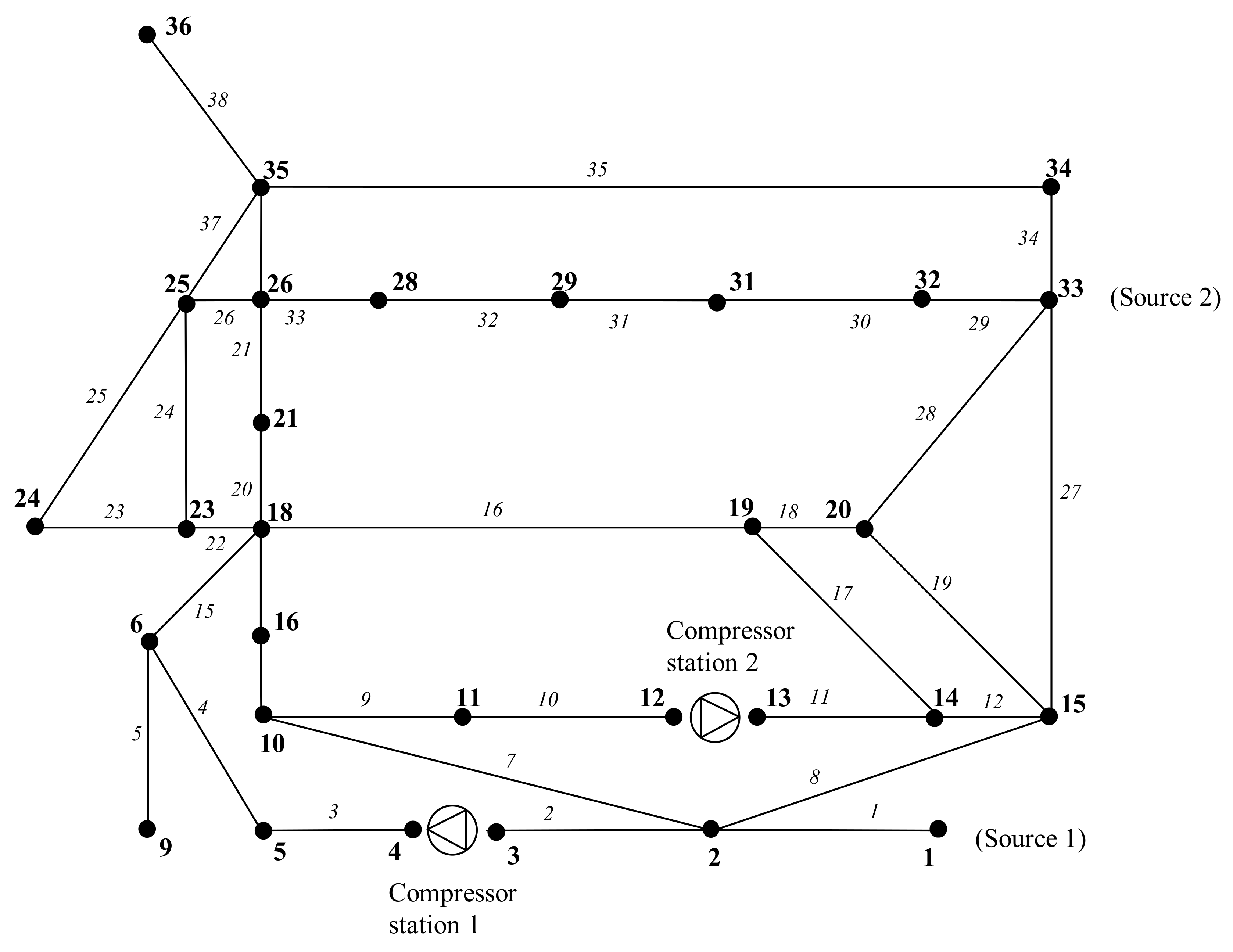
The first problem consists of a network of 39 pipes, 38 nodes, 2 compressor stations, 2 sources, and 1 valve (Figure 2). There are also 20 loaded nodes. This represents a part of the National Transmission System. All the pipes have the same diameter equal to 0.9144 m (36 inches). One of the requirements in this problem is that pressure at nodes 9, 23, and 34 cannot drop below 5.5, 5.4, and 5.5 MPa, respectively. The lengths of the pipes are given in

Table 1. Pipe lengths.

Pipe No.	Length (m)	Pipe No.	Length (m)
1	50·103	21	75·103
2	35·103	22	55·103
3	20·103	23	65·103
4	80·103	24	80·103
5	85·103	25	50·103
7	60·103	26	35·103
8	150·103	27	80·103
9	35·103	28	60·103
10	45·103	29	40·103
11	65·103	30	50·103
12	70·103	31	60·103
13	85·103	32	55·103
14	60·103	33	60·103
15	95·103	34	80·103
16	40·103	35	50·103
17	20·103	36	90·103
18	65·103	37	75·103
19	55·103	38	80·103
20	45·103

. The nodal loads are given in

Table 2. The nodal loads.

Node No.	Load (m3/h)	Node No.	Load (m3/h)
2	117,987	20	117,987
5	“	23	“
6	“	24	“
9	“	25	“
10	“	26	“
11	“	29	“
14	“	32	“
15	“	34	“
18	“	35	“
19	“	36	“

. Compressor station constraints and source constraints are given in

Table 3. Compressor station constraints.

Compressor Station No.	Max. Discharge Pressure (bar)	Max. Compressor Ratio
Compressor station 1	60.0	1.5
Compressor station 2	“	1.5

and in

Table 4. Source constraints.

Source No.	Max. Pressure (bar)	Max. Flow (m3/h)
Source 1	60.0	2,420,000.0
Source 2	60.0	2,420,000.0

, respectively. The results of optimization are presented in

Table 5. The nodal pressures.

Node No.	Pressure (Pa)	Node No.	Pressure (Pa)
2	4,934,279.4	20	5,509,743.8
3	4,722,864.3	21	5,390,402.6
5	5,810,845.2	23	5,400,502.3
6	5,524,732.6	24	5,365,839.6
9	5,519,327.1	25	5,403,114.7
10	4,925,286.3	26	5,445,346.7
11	4,824,920.5	28	5,421,142.6
12	4,848,617.1	29	5,465,560.0
14	5,454,098.4	31	5,524,985.8
15	5,325,629.4	32	5,570,129.7
16	5,195,366.6	34	5,551,397.3
18	5,428,836.1	35	5,434,898.4
19	5,239,052.6	36	5,370,022.2

,

Table 6. Pipe flows.

Pipe No.	Flow (m3/h)	Pipe No.	Flow (m3/h)
1	271,082.3	21	−26,618.4
2	719,185.8	22	113,384.2
3	721,285.8	23	40,221.6
4	604,898.8	24	−46,144.3
5	120,987.0	25	76,245.4
7	−2044.2	26	132,423.9
8	559,513.3	27	531,608.2
9	412,301.9	28	571,232.3
10	291,814.9	29	462,338.5
11	291,814.9	30	342,951.5
12	−58,818.6	31	342,951.5
13	521,966.1	32	224,364.5
14	521,966.1	33	224,364.5
15	371,024.8	34	511,078.7
16	361,194.1	35	392,391.7
17	232,146.5	36	−51,164.8
18	239,634.5	37	196,752.9
19	203,210.7	38	116,487.0
20	−26,618.4

,

Table 7. Changes in objective function during the optimization process.

The Number of Iteration	Objective Function (kW)
1	13,212.2
3	12,892.4
5	12,622.4
7	12,382.8
9	12,172.4
11	12,032.6
13	11,922.5
15	11,862.7

,

Table 8. Optimal parameters of work for compressor stations.

Compressor Station No.	Suction Pressure (bar)	Discharge Pressure (bar)	Flow (m3/h)	HP (kW)
Compressor station 1	46.32	59.21	722,285.8	5423.14
Compressor station 2	47.13	54.26	292,114.9	1431.08

and

Table 9. Optimal parameters of work for sources.

Source No.	Output Pressure (Bar)	Flow (m3/h)
Source 1	50.0	273,482.3
Source 2	56.8	2,064,157.7

.

The results of optimization are presented in Table 5, Table 6, Table 7, Table 8 and Table 9.

Convergence was obtained in 35 SQP, 57 conjugate gradients, and 130 Newton iterations. Twenty-seven seconds of CPU time were used.

6.2. Large Network

The second problem consists of a network of 95 nodes, 890 pipes, and 32 nonpipe elements. This represents the southern part of the National Transmission System.

Convergence was obtained in 85 SQP, 163 conjugate gradients, and 324 Newton iterations. One hundred twenty units of CPU time were used.

7. Results

The results obtained for its applications in the two gas network problems seem encouraging. The calculations confirm the correctness of the developed algorithm. During the calculation process, all constraints imposed on the maximum compressor ratio for compressor stations and minimum pressure at nodes 9, 23, and 34 were taken into account, and the goals function decreased. Fifteen iterations were necessary to find the optimal solution (for the small network), which turned out to be cheaper by over 10% (10% lower power consumption in compressor stations). The developed algorithm meets the criteria of accuracy together with relatively short computation time. The validity of the solutions was checked by comparing solutions with those from the simulation program run with appropriate control values. It was verified that equations of gas flow were in fact satisfied. It should be noted that the simulation program used by the gas network operator is very well established and validated.

It should be remembered that the optimization results will depend on many factors, including the structure of the network (tree or looped structure), the capacity of the pipelines, the number of compressor stations, and the distance between them.

The relationship between pressures and flows in any given application that employs gas compressors, as well as some other factors, may influence the arrangement of compressors in a station as well as the type of equipment used. Different concepts such as the number of units installed, regarding both their impact on the individual station and the overall pipeline, are important. The number of compressors installed in each compressor station of a pipeline system has a significant impact on the availability, fuel consumption, and capacity of the system. Depending on the load profile of the station, the answers may look different for different applications. The operating point of a compressor is determined by a balance between available driver power, the compressor characteristic, and the system behavior. The point on the map at which the compressor actually operates is determined by the behavior of the system, that is, by the relationship between head (pressure ratio) and flow enforced by the system.

8. Conclusions

The goal of a pipeline optimizer is to be able to model a variety of pipeline configurations robustly and efficiently and to ensure feasible and optimal operating strategies according to a specified objective function and constraints imposed on the pipeline system. In this paper, we have discussed the application of the sequential quadratic programming (SQP) method to the problem of steady-state optimization of the operation of a gas pipeline network to minimize the running cost of the system. The optimal solution satisfies all the constraints imposed by the limitations of the pipeline and the compressors’ operating ranges. An evaluation of the method was performed by testing on two different pipeline configurations. Results presented for the network demonstrate the correctness of the optimizer (Kirchhof’s first and second laws and the flow equation are fulfilled) and expected savings. The algorithm described is suitable for a general class of large nonlinearly constrained steady-state optimization problems. The flexibility of the algorithm enables us to perform various assessments for a given problem and optimize the problem according to the formulation of the objective function. The case study clearly indicates the effectiveness and ease of use in the actual application of the developed and implemented methodology. The developed algorithm proved to be much more efficient than the algorithm based on the generalized reduced gradient method. GRD algorithm described in [24] required much more computation time and a bigger number of iterations to obtain the optimal result. It would be interesting to test a general-purpose optimization package on the same problems. The next stage for the steady-state optimization algorithm is its adaptation for the transient flow model. An algorithm for optimal control over a period of up to a day will use the SQP method.

References

- Barclay, A.; Gill, P.E.; Rosen, J.B. SQP methods and their application to numerical optimal control. In Variational Calculus, Optimal Control and Applications; Birkhäuser: Basel, Switzerland, 1998; pp. 207–222. [Google Scholar]
- Boggs, P.T.; Tolle, J.W. Sequential Quadratic Programming. Acta Numer. 1996, 4, 1–52. [Google Scholar] [CrossRef] [Green Version]
- Carter, R.G. Pipeline Optimization: Dynamic Programming After 30 Years. In Proceedings of the PSIG Annual Meeting, Denver, CO, USA, 28–30 October 1998. [Google Scholar]
- De Wolf, D.; Smeers, Y. The gas transmission problem solved by an extension of the sim-plex algorithm. Manag. Sci. 2000, 46, 1454–1465. [Google Scholar] [CrossRef] [Green Version]
- Domschke, P.; Geißler, B.; Kolb, O.; Lang, J.; Martin, A.; Morsi, A. Combination of non-linear and linear optimization of transient gas networks. INFORMS J. Comput. 2011, 23, 605–617. [Google Scholar] [CrossRef] [Green Version]
- Enbin, L.; Liuxin, L.; Qian, M.; Jianchao, K.; Zhang, L. Steady—State Optimization Opera-tion of the West-East Gas Pipeline. Adv. Mech. Eng. 2019, 11, 1–14. [Google Scholar]
- Ehrhardt, K.; Steinbach, M.C. Non-linear optimization in gas networks. In Modeling, Simulation and Optimization of Complex Processes; Bock, H.G., Ed.; Springer: Berlin/Heidelberg, Germany, 2005; pp. 139–148. [Google Scholar]
- Furey, B.P. A Sequential Quadratic Programming Based Algorithm for Optimization of Gas Networks. Automatica 1993, 29, 1439–1450. [Google Scholar] [CrossRef]
- Herty, M. Modeling, simulation and optimization of gas networks with compressors. Netw. Heterog. Media 2007, 2, 81–97. [Google Scholar] [CrossRef]
- Krishnaswami, P.; Chapman, K.S.; Abbaspour, M. Compressor station optimization for linepack maintenance. In Proceedings of the 36th PSIG Annual Meeting, Palm Springs, CA, USA, 20–22 October 2004; p. PSIG-0410. [Google Scholar]
- Larson, R.E.; Wismer, D.A. Hierarchical control of transient flow in natural gas pipe-line networks. In Proceedings of the IFAC Symposium on Distributed Parameter Systems, Banff, AB, Canada, 21–23 June 1971. [Google Scholar]
- Luongo, C.A.; Gilmour, B.J.; Schroeder, D.W. Optimization in Natural Gas Transmission Networks: A Tool to Improve Operational Efficiency. In Proceedings of the 3rd SIAM Con-ference on Optimization, SIAM, Boston, MA, USA, 3–5 April 1989; pp. 110–117. [Google Scholar]
- Mahlke, D.; Martin, A.; Moritz, S. A mixed integer approach for time-dependent gas network optimization. Optim. Methods Softw. 2010, 25, 625–644. [Google Scholar] [CrossRef]
- Mallinson, J.; Fincham, A.; Bull, S.; Rollet, J.; Wong, M. Methods for optimizing gas transmission networks. Ann. Oper. Res. 1993, 43, 443–454. [Google Scholar] [CrossRef]
- Moritz, S. A Mixed Integer Approach for the Transient Case of Gas Network Optimization. Ph.D. Thesis, Darmstadt University of Technology, Darmstadt, Germany, 2007. [Google Scholar]
- Nocedal, J.; Wright, S.J. Numerical Optimization; Springer: New York, NY, USA, 2006. [Google Scholar]
- O’Malley, C.; Kourounis, D.; Hug, G.; Schenk, O. Optimizing Gas Networks Using Adjoint Gradients; Project Nr 18801.1, PFIW-IW; Commision for Technology and Innovation: Geneva, Switzerland, 2014. [Google Scholar]
- Osiadacz, A.J. Non-linear programming applied to the optimum control of a gas compressor station. Int. J. Numer. Methods Eng. 1980, 15, 1287–1301. [Google Scholar] [CrossRef]
- Osiadacz, A.J. Dynamic optimization of high pressure gas networks using hierarchical systems theory. In Proceedings of the 26th PSIG Annual Meeting, San Diego, CA, USA, 1 January 1994; p. PSIG-9408. [Google Scholar]
- Osiadacz, A.J. Hierarchical control of transient flow in natural gas pipeline systems. Int. Trans. Oper. Res. 1998, 5, 285–302. [Google Scholar] [CrossRef]
- Osiadacz, A.J.; Bell, D.J. A simplified algorithm for optimization of large-scale gas networks. Optim. Control. Appl. Methods 1986, 7, 95–104. [Google Scholar] [CrossRef]
- Osiadacz, A.J.; Swierczewski, S. Optimal control of gas transportation systems. In Proceedings of the IEEE International Conference on Control and Applications CCA-94, Glasgow, UK, 24–26 August 1994; Volume 2, pp. 795–796. [Google Scholar]
- Osiadacz, A.J. Simulation and Analysis of Gas Networks; F.N Spon Ltd.: London, UK, 1987. [Google Scholar]
- Osiadacz, A.J. Steady-State Optimization of Gas Networks. Arch. Min. Sci. 2011, 56, 335–352. [Google Scholar]
- Osiadacz, A.J.; Chaczykowski, M. Compressor Fuel Minimization Under Transient Conditions. In Proceedings of the PSIG Annual Meeting, Atlanta, GA, USA, 9–12 May 2017. [Google Scholar]
- Percell, P.B.; Ryan, M.J. Steady-state optimization of gas pipeline network operation. In Proceedings of the 19th PSIG annual meeting, Tulsa, OK, USA, 22 October 1987. [Google Scholar]
- Powell, M.J.D. Algorithms for non-linear constraints that use Lagrangian functions. Math. Program. 1978, 14, 224–248. [Google Scholar] [CrossRef]
- Ríos-Mercado, R.Z.; Borraz-Sánchez, C. Optimization problems in natural gas trans-portation systems: A state-of-the-art review. Appl. Energy 2015, 147, 536–555. [Google Scholar] [CrossRef]
- Saunders, M. Large scale Numerical Optimization: SQP Methods; Stanford University: Stanford, CA, USA, 2019. [Google Scholar]
- Sedliak, A.; Žáčik, T. Optimization of the Gas Transport in Pipeline Systems. Tatra Mt. Math. Publ. 2016, 66, 103–120. [Google Scholar] [CrossRef] [Green Version]
- Steinbach, M.C. On PDE solution in transient optimization of gas networks. J. Comput. Appl. Math. 2007, 203, 345–361. [Google Scholar] [CrossRef] [Green Version]
- Tran, T.H.; French, S.; Ashman, R.; Kent, E. Linepack planning models for gas trans-mission network under uncertainty. Eur. J. Oper. Res. 2018, 268, 688–702. [Google Scholar] [CrossRef] [Green Version]
- Crane Co. Flow of Fluids through Valves, Fittings and Pipe. Technical Paper 40 (TP-40). 1988. Available online: http://www.craneco.com (accessed on 7 May 2021).
- Gas Processors Suppliers Association (GPSA). Engineerin Data Book, 11th ed.; Gas Processors Suppliers Association (GPSA): Tulsa, OK, USA, 1998. [Google Scholar]
- Transco’s National Transmission System, Review of System Operator Incentives, Proposal Dokument. February 2004. Available online: www.ofgem.gov.uk (accessed on 7 May 2021).
- Luongo, C.A.; Gilmour, B.J.; Schroeder, D.W. Optimization in Natural Gas Transmission Net-Works. A Tool to Improve Operating Efficiency; Technical Report; Stoner Associates, Inc.: Houston, TX, USA, 1989. [Google Scholar]
- Menon, E.S. Gas Pipeline Hydraulics; CRC Press, Taylor & Francis Group: Oxford, NY, USA, 2005. [Google Scholar]
- Kralik, J.; Stiegler, P.; Vostry, Z.; Zavorka, J. Dynamic Modeling of Large Scale Networks with Application to Gas Distribution; Academia: Prague, Czech Republic, 1988. [Google Scholar]
Figure 1.
Typical compressor envelope.
Figure 2.
Structure of the network.