Molecular Dynamics Study on Water Flow Behaviour inside Planar Nanochannel Using Different Temperature Control Strategies

Abstract

In the present paper, molecular dynamics simulations were performed to study the influence of two temperature control strategies on water flow behaviour inside planar nanochannel. In the simulations, the flow was induced by the force acting on each water molecule in the channel. Two temperature control strategies were considered: (a) frozen wall simulations, in which the dynamics of confining wall atoms was not solved and the thermostat was applied to the water, and (b) dynamic wall simulations, in which the dynamics of confining wall atoms was solved, and the thermostat was applied to walls while water was simulated in the microcanonical ensemble. The simulation results show that the considered temperature control strategies has no effect on the shape of the water flow profile, and flow behaviour in the channel is well described by the Navier–Stokes equation solution with added slip velocity. Meanwhile, the slip velocity occurring at the boundaries of the channel is linearly dependent on the magnitude of the flow inducing force in both frozen wall and dynamic wall simulations. However, the slip velocity is considerably greater in simulations when the wall dynamics are solved in contrast to the frozen wall simulations.

1. Introduction

Advances in micro-and nanotechnology over the last decades paved the way for the development of new nanofluidic devices, in which the channel dimensions are less than 100 nm [1]. In such devices, novel and unique features emerge, as the channel dimensions are in the same order as the Debye length, the characteristic length of various biomolecules (DNR, protein, etc.), and even the lengths of intermolecular interactions in fluids. Such device features have promising applications in various scientific fields, including micro-electronic device cooling [2,3,4], water filtration and salinification [5], biomedicine and biosensing [6], fluid-based electronics, and energy storage and conversion [7].

The development of nanofluidic devices based on nanoscale heat and mass transfer requires precise knowledge of fluid behaviour in nanoscale and fluid molecular interactions with the solids at the interface. However, as the lengths of the channels approach nanoscale, a novel physical behaviour of the fluids occurs, related to the discrete nature of fluids, high surface-to-volume ratios, local density and temperature fluctuations, and the variations of local viscosity within the channels [8,9,10]. Furthermore, the fluid properties near the channel walls deviate from bulk behaviour due to the fluid–solid interactions, and the classic continuum theory does not directly apply at liquid–solid interface [10,11]. For these reasons, the fluid flow behaviour and flow parameters in various nanoconfinements (such as tubes and channels) have become a subject of molecular dynamics (MD) simulation research, as the MD simulation technique provides powerful predictive capabilities while the experimental methods still face challenges related to nanoscale measurement.

In the MD simulations, the classical equations of motion for each atom/molecule of the molecular many-body system are numerically solved, while the intermolecular interactions are described by effective interaction potentials in order to obtain molecular trajectories, which can be used to obtain macroscopic properties of the system using statistical analysis methods [12]. Many of the MD simulations studies were performed to investigate the confinement wall roughness [13,14,15,16,17,18,19], various solid wettability and liquid–solid interaction type [5,10,20,21,22,23,24,25,26,27,28,29,30,31,32,33,34], confinement size [5,29,35,36,37], flow shear rate [24,38,39], and various confinement shape, and entrance/exit [40,41,42] effects on fluid behaviour in nanoconfinements. In recent years, much effort was also put to study flow behaviour in nanochannels with the presence of nanoparticles as the solid nanoparticles improve the thermal characteristics of fluids [15,43,44,45,46,47,48].

An important aspect of confined flow MD simulations is temperature control in the system, which is required to compensate for viscous heating due to viscous forces in the flow and to maintain the required simulation conditions during simulations. The temperature of the simulated system (or the part of the system) can be controlled with so-called thermostat algorithms, which directly or indirectly affect the movement of the system molecules [49]. Furthermore, confined flow simulations have two main flow temperature control strategies [50]: (1) applying the thermostat directly to the fluid flow or (2) extracting heat through the confinement walls, which are maintained at a constant temperature. However, the effects of the temperature control algorithms in MD simulations (the thermostats) and temperature control strategies have not been fully examined to date, although it is important for flow development, especially when the heat transfer is considered, for example, in fluid-based cooling applications. Furthermore, the choice of the thermostat on its own influences the dynamic properties of the bulk fluid in simulations, such as self-diffusivity and shear viscosity [51]. Further complications arise in simulations when the flows are induced in highly confined fluids.

As mentioned above, there are two temperature control strategies commonly used in nanoconfined flow MD simulations. In the first strategy, the flow temperature is maintained constant by applying the thermostat [50], which extracts the excess energy generated in the simulations by the viscous heating directly to the fluid, while the dynamics of wall atoms are not solved, i.e., the positions of wall atoms are fixed-in throughout the simulations. This strategy has drawbacks as the thermostat affects the movement of the fluid molecules and, consequently, the dynamic properties of the fluid.The flow is also treated as an isothermal flow with infinite thermal conductivity of the fluid. Furthermore, the fluid–solid molecular interactions at the interface are not really captured, as the dynamics of confinement wall atoms is not solved (the atom positions are frozen), and there is no momentum exchange between liquid and solid molecules/atoms. However, this strategy is commonly used for MD simulations due to the reduced computational costs related with neglecting the dynamics of wall atoms.

The more realistic nanoconfined flow simulation conditions (i.e., conditions closer to experimental ones), especially when simulating mass and heat transfer processes in cooling scenarios, can be achieved by applying thermostat to confinement wall atoms, while simulating the fluid at constant energy, i.e., in microcanonical (NVE) ensemble. Thus, the flow is not treated as isothermal, and the generated heat is extracted from the simulation by the heat conduction from the fluid to the confinement walls. This allows us to obtain the realistic temperature profiles across the flow in the simulations and more realistically capture the momentum exchange between fluid and confinement walls at the interface.

A limited number of papers has been published in which the effects of temperature control strategies on nanoconfined flow behaviour were studied in detail. In the study of Kim et al. [52], the MD simulations of 2D Couette flow of Lennard-Jones (LJ) fluid between two parallel solid plates were performed, in which the fluid thermal interactions with the solid thermostated walls were accomplished by connecting the solid atoms to the lattice positions with harmonic bonds. Their results showed that the parabolic temperature profiles were present in the flow, which suggest non-uniform viscosity across the channel. Bernardi et al. [53] studied the influence of temperature control strategies on the highly confined Couette flow of LJ fluid. They concluded that, regardless of the choice of thermostat, the fluid mechanical properties differ in simulations when the thermostat is applied to the confinement walls in contrast to simulations in which the confinement walls were held fixed, and the thermostat was applied to fluid. Yong and Zhang [50] performed MD simulations of LJ fluid Couette flows in order to investigate effects of the different temperature control strategies on the flow. They applied a thermostat to either the fluid (TF), the confinement solid walls (TW), and both on the fluid and the walls (TWTF). They observed that TF and TWTF strategies produce considerably similar flow behaviours in weakly sheared systems; however, the dynamic properties deviate in strongly sheared systems due to the isothermal condition. Thomas and Corry [54] tested a variety of thermostats in their water flow through carbon nanotube (CNTs) simulations, and inspected the flow rates and tube permeabilities. Their results showed that the disagreements between simulation results could be caused by variety of thermostat methods used to control simulation temperature as the thermostat choice can change the flow rate and tube permeability up to five times. Sam et al. [55] studied the influences of temperature control strategies in water flow in CNTs by performing MD simulations. The temperature was controlled via fluid when the CNT walls were rigid or via flexible CNT walls. Their simulation results showed that the flow velocities and mass flow rates depended on the tube flexibility and the temperature control strategy, with up to 20% larger flow rates when the CNT walls were flexible.

In summary, the literature review shows that the flow of water and other fluids inside nanoconfinements is common MD research object; however, the is no information published on the effects of temperature control strategies on flow behaviour of water inside planar nanochannel. Therefore, we used the MD simulations to examine the effects of fixed wall and dynamic wall temperature control strategies on Poiseuille flow of water in a planar copper nanochannel (the detailed description for the strategies is given in following section). From the simulation results, we obtained the dependencies of flow profiles, mean flow velocity, and slip velocity on flow inducing force for both temperature control strategies.

2. Simulation Method

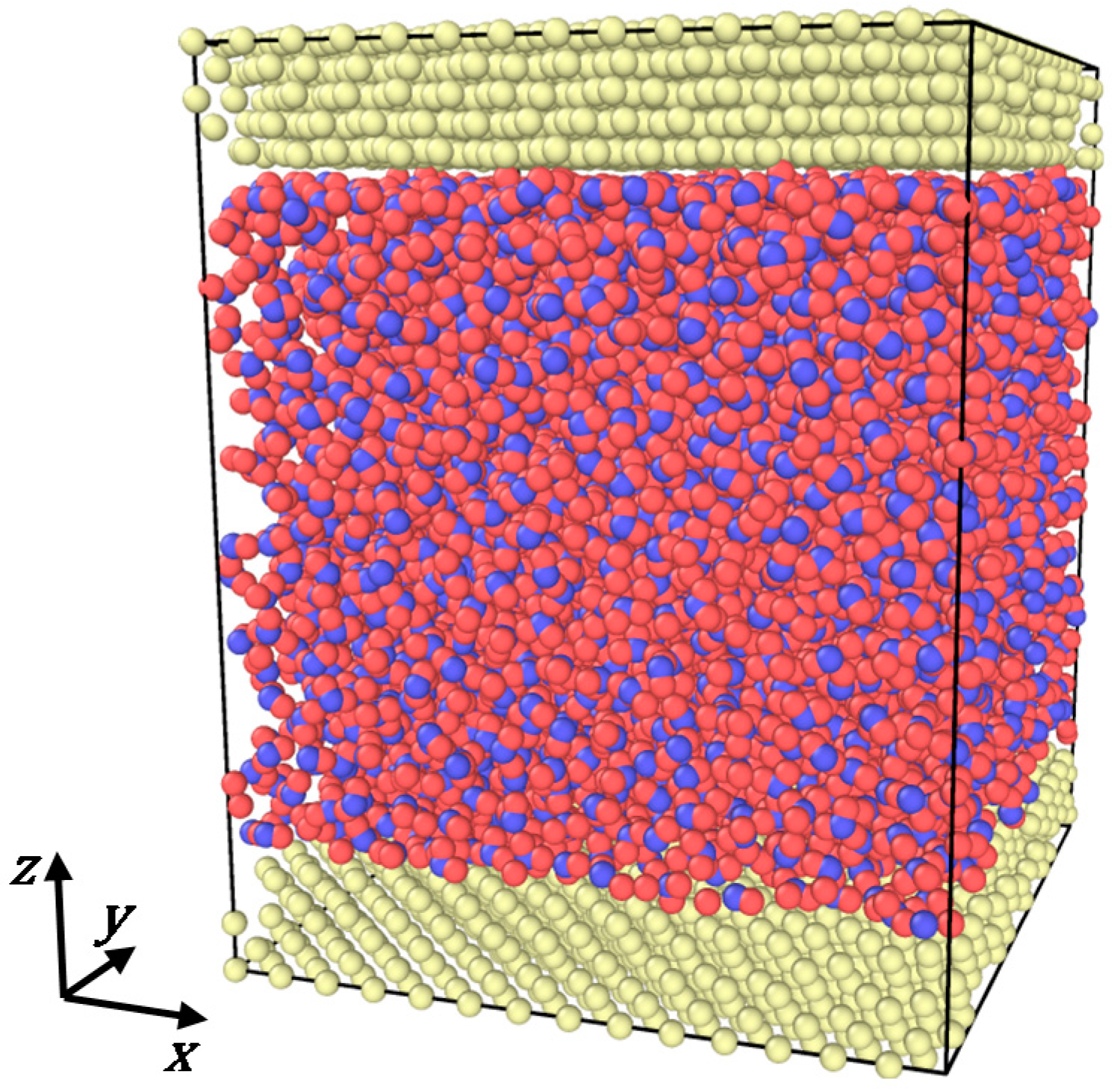
2.1. Poiseuille Flow Simulation Details

The Poiseuille flow of water confined in planar nanochannel was induced in our MD simulations by applying three different values of constant external force in the x-direction on every water molecule: $f_x=\left\{1.77;2.65;3.53\right\}\times {10}^{12} \mathrm{N}/\mathrm{kg}$. The visual representation of the simulated system is shown in Figure 1.The periodic boundary condition was applied to the x and y axes. The number of water molecules in simulations was 4148. Each channel wall was made of 1960 copper atoms plad in face-centred cubic (FCC) lattice nodes (lattice constant a = 3.67 Å). The water molecules initiay placed between the channel walls as an ice XI crystal was allowed to melt and fill the unoccupied space in the first stage of simulations. The channel width (the distance between two atomistic planes of bottom and top copper walls, which are in contact with water) is 50 Å. The initial molecular velocity components in the x, y, and z directions for each atom were randomly assigned from the Gaussian distribution. The magnitude of the flow inducing force was chosen in such a way that would provide a high signal-to-noise ratio in the induced flow profiles obtained from MD simulations [56].

The interactions between water molecules were described by SPC/E intermolecular model [57] with the cut-off distance $r_c$ = 10 Å. The potential energy for SPC/E interaction model is given as follows:

$$U\left(r_{ij}\right)=4{\epsilon }_{ij}\left[{\left(\frac{{\sigma }_{ij}}{r_{ij}}\right)}^{12}-{\left(\frac{{\sigma }_{ij}}{r_{ij}}\right)}^6\right]+\frac{q_i{q}_j}{4\pi {\epsilon }_0{r}_{ij}},$$

(1)

where ${\epsilon }_{ij}$, ${\sigma }_{ij}$, $q_i$, $q_j$, and ${\epsilon }_0$ are the depth of the Lennard-Jones (LJ) potential well of i-th and j-th atom interaction, the length parameter of LJ interaction between i-th and j-th atoms, the charge of the i-th atom, the charge of the j-th atom, and vacuum permeability, respectively. The parameter values for SPC/E water model can be found in ref. [57] and are listed in

Table 1. Parameter values for SPC/E water model.

${\sigma }_{OO},\mathsf{\AA }$	$3.166$
${\epsilon }_{OO},\mathrm{kcal}/\mathrm{mol}$	$0.1554$
$q_H,e$	$+0.4238$
$q_O,e$	$-2q_h$

. The long-range electrostatic interactions beyond the cut-off distance were handled by the Particle–particle particle–mesh (PPPM) method with the accuracy of 2 × 10⁻⁵ [58]. To avoid unphysical slab–slab interactions, the system was treated as periodic in z-direction; however, an empty volume was inserted between the channel walls and dipole inter-slab interactions were removed. The length of the added empty volume in z-direction was three times the length of the simulation box length in the same direction. The rigid bond and angle constraints of water molecules were realised using SHAKE algorithm with accuracy tolerance of ${10}^{-4}$. The Newtonian equations of motion of molecules were solved using the Verlet method with integration timestep $\Delta t$ = 1 fs. The copper-copper atomic interactions in channel walls were described using EAM interatomic potential for copper [59]. Furthermore, only the oxygen atoms interacted with copper wall atoms via LJ potential with parameter values of ${\sigma }_{CuO}=0.87\mathsf{\sigma }$ and ${\epsilon }_{CuO}=1.70\epsilon$ [10]. Simulations were performed using LAMMPS molecular dynamics code [60].

The simulations were performed in three stages:

• First equilibration stage: In this stage, the simulations began from the initial configuration and continued for 0.4 ns, during which the system reached a thermal equilibrium state at 303 K temperature. Water and solid walls were simulated in canonical (NVT) ensemble.
• The second equilibration stage: After equilibrium state was reached, the flow inducing force in the x-direction was applied to each water molecule, and the simulation continued for another 0.4 ns. During this stage, the moving average of the mean flow velocity in time reached constant value (with slight fluctuations), and the system reached steady flow state. The temperature of the water during the flow (in current and the following simulations stages) was maintained at 303 K according to the temperature control strategy used in the simulation.
• The MD run: After the second equilibration run, the MD run stage was performed for 12 ns with force still applied to the water molecules to maintain the steady flow state in the system. During this stage, the atomistic data was sampled for statistical analysis of the system during steady flow.

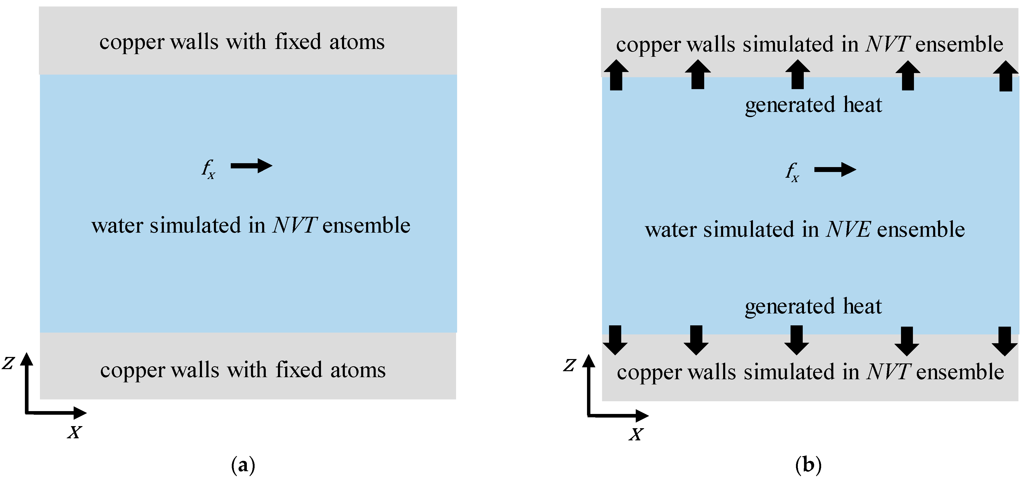
2.2. Temperature Control Strategies

The two types of water temperature control strategies were considered during simulations stages with the induced flow to investigate their influence on water flow behaviour in a planar nanochannel. In frozen wall (FW) simulations (Figure 2 case a), the heat generated in the system by flow inducing force was extracted by applying thermostat directly to water molecules (water was simulated in canonical NVT ensemble), while the positions of copper atoms were frozen during simulations. In dynamic wall (DW) simulations (Figure 2 case b), water was simulated in a microcanonical NVE ensemble and the generated heat by the external force was removed through the heat conduction to the copper walls, which were maintained at constant temperature with a thermostat (i.e., the copper walls were simulated in canonical NVT ensemble).

The constant temperature in the simulated system was controlled using Nosé–Hoover thermostat, which maintains the targeted temperature in the system (or the specific parts of the system) by adding friction term to the Newtonian equations of motion as follows [55]:

$$m_i\frac{d^2}{{\mathit{dt}}^2}{r}_i(t)=F_i(r_i)-m_i\xi {\tilde{v}}_i,$$

(2)

$$\dot{\xi }=\frac{1}{Q}\left[{{\displaystyle \sum }}_{i=1}^N{m}_i{\tilde{v}}_i·{\tilde{v}}_i-\left(6N+1\right)k_{B}T\right],$$

(3)

where $m_i$ is the mass of i-th atom, $r_i$ is the position vector of i-th atom, ${\tilde{v}}_i=v_i-u\left(r_i\right)$ is the thermal velocity of i-th atom, $v_i$ is the total velocity of i-th atom, $u\left(r_i\right)$ is the local streaming velocity of i-th atom, $F_i$ is the force acting on i-th atom, $Q$ is the mass of the “fictitious” heat bath, $k_B$ is the Boltzmann constant, and $T$ is the targeted temperature. The term $Q$ is determined by the effective relaxation time [49], which in our simulations was set to $\tau =0.2 \mathrm{ps}$. In cases when the thermostat was applied directly on water, a velocity profile unbiased temperature control condition was achieved by dividing the simulation box into 50 spatial bins perpendicular to the z-axis and calculating the instantaneous local streaming velocity as the centre of mass velocity of the atoms located within each bin [50].

The instantaneous temperature of the whole system or the part of the system is evaluated as [15]:

$$T\left(t\right)={\displaystyle \sum }_1^N\frac{m_i{v}_i^2\left(t\right)}{3k_B},$$

(4)

where $m_i$ and $v_i$ are the mass and instantaneous velocity of i-th atom/molecule, and $N$ is the number of atoms/molecules in the system or the part of the system.

3. Results and Discussion

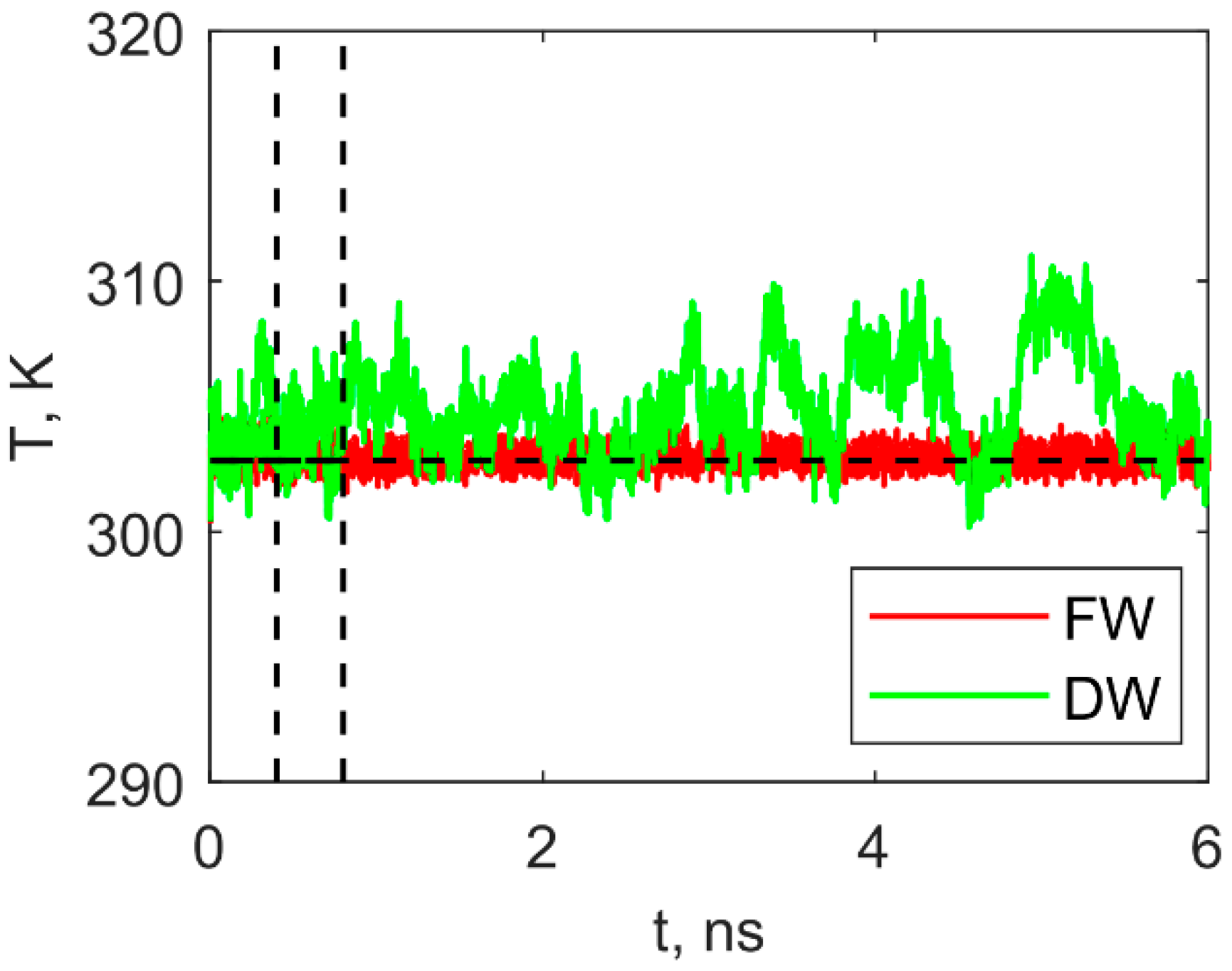
3.1. Simulation Temperature

We begin by examining the effectiveness of heat extraction methods in the nanoconfined flow simulations. The temperature–time evolutions in both FW and DM simulations with the flow inducing force of $f_x=3.53\times {10}^{12}\mathrm{N}/\mathrm{kg}$ are shown in Figure 3. The temperature evolutions show that water temperature remained constant with slight temporal fluctuations in FW simulations after the flow was induced. In the case of DW simulation, the water temperature started to rise when the flow was induced at the beginning of the second equilibration stage. Furthermore, the temporal temperature fluctuations were considerably greater than in FW simulation, and the average temperature of the water was higher by almost $2 \mathrm{K}$ than the targeted simulation temperature of 303 K as the water was not able to transfer generated heat to the copper walls instantly. The simulation average temperatures of walls and liquid water are given in

Table 2. Simulation average temperatures for FW and DW simulations with different magnitudes of flow inducing force $f_x$.

$\mathbf{The}\mathbf{Magnitude}\mathbf{of}\mathbf{the}\mathbf{Flow}\mathbf{Inducing}\mathbf{Force}{\mathit{f}}_{\mathit{x}}\times {10}^{12},\mathbf{N}/\mathbf{k}\mathbf{g}$	FW Simulations		DW Simulations
	$\mathbf{Temperature}\mathbf{of}\mathbf{Walls}{\mathit{T}}_{\mathit{w}\mathit{a}\mathit{l}\mathit{l}},\mathbf{K}$	$\mathbf{Temperature}\mathbf{of}\mathbf{Water}{\mathit{T}}_{\mathit{w}\mathit{a}\mathit{t}\mathit{e}\mathit{r}},\mathbf{K}$	$\mathbf{Temperature}\mathbf{of}\mathbf{Walls}{\mathit{T}}_{\mathit{w}\mathit{a}\mathit{l}\mathit{l}},\mathbf{K}$	$\mathbf{Temperature}\mathbf{of}\mathbf{Water}{\mathit{T}}_{\mathit{w}\mathit{a}\mathit{t}\mathit{e}\mathit{r}},\mathbf{K}$
1.77	0	303.00	302.85	303.19
2.65	0	303.00	302.87	304.06
3.53	0	303.00	302.84	304.99

.

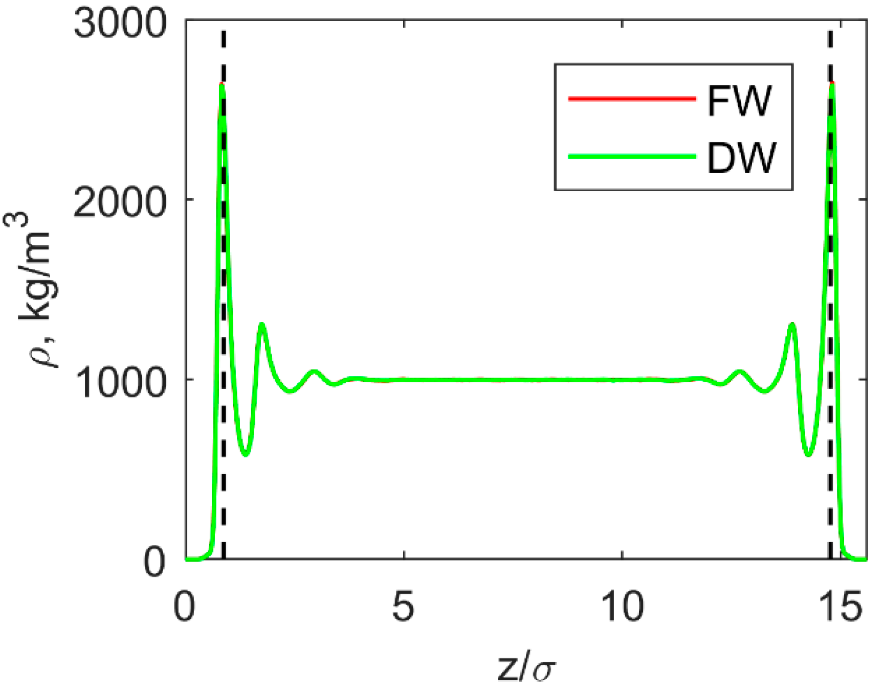
3.2. Water Density Profiles

The water density profiles along z-axis obtained from FW and DW simulations with the flow inducing force of $f_x=3.53\times {10}^{12} \mathrm{N}/\mathrm{kg}$ are given in Figure 4. The density profiles were calculated by dividing simulation cells into spatial bins (with a bin width of $0.1 \mathsf{\AA }$) parallel to the x–y plane, and the length in z-direction was measured in terms of $\sigma ={\sigma }_{OO}$. The density profile in the channel exhibits decaying fluctuations in near-wall regions and reaches the constant value in the bulk region of the channel. The density profiles from FW and DW simulations almost completely overlap, indicating that solving the dynamics of copper walls had no significant effect on the density profile compared to the FW simulations. Furthermore, the first two density peaks were located at distances ${\sigma }_{CuO}$ and $2{\sigma }_{CuO}$ from the atomistic planes of copper walls, while the distance in which the fluctuating behaviour persisted into the channel was around $4{\sigma }_{CuO}$. Such oscillatory behaviour in density profiles can be explained by correlated effects of long-range molecular attraction and short-range repulsion between copper and oxygen atoms, and was observed not only in nanoconfined water flow simulations [56,61] but also in flow simulations of LJ fluids [28,32], CO₂, and n-octanes [62].

It is also worth noting that, even though the channel width was $H=50 \mathsf{\AA }$, the water molecules could not occupy the whole volume due to the repulsion of copper atoms in the walls, and the density sharply declined to zero as the distance from the copper walls decreased at the interface. Thus, we considered that the real channel boundaries were at the highest density peak locations. In this case, the actual width of the channel (the distance between the highest density peaks) was approximately $H=44 \mathsf{\AA }$ (or 13.90$\sigma$).

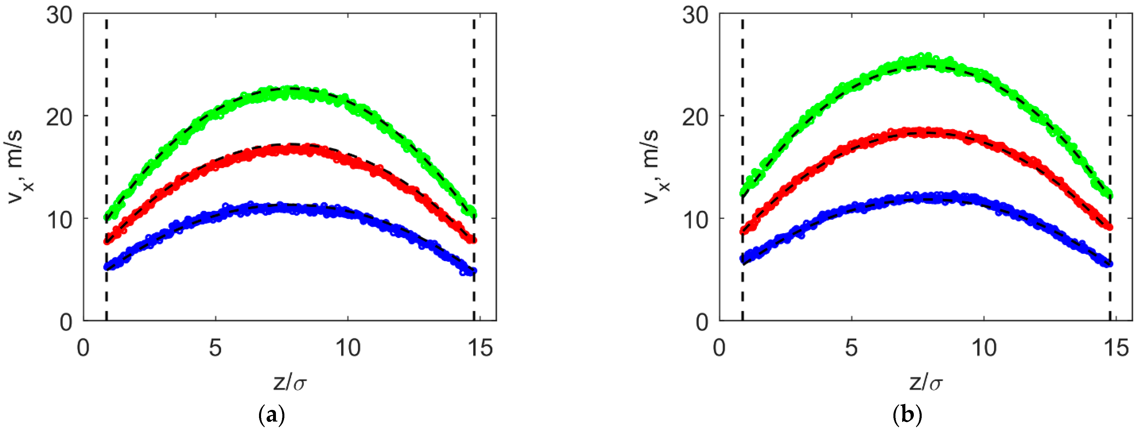
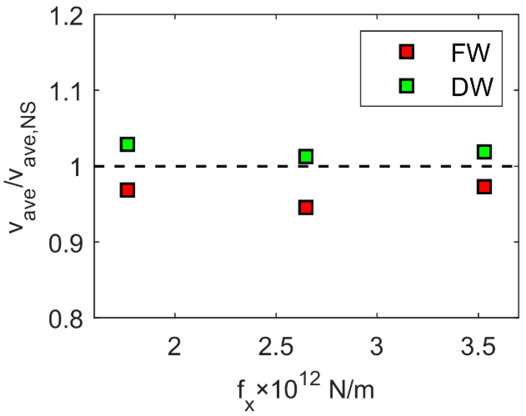
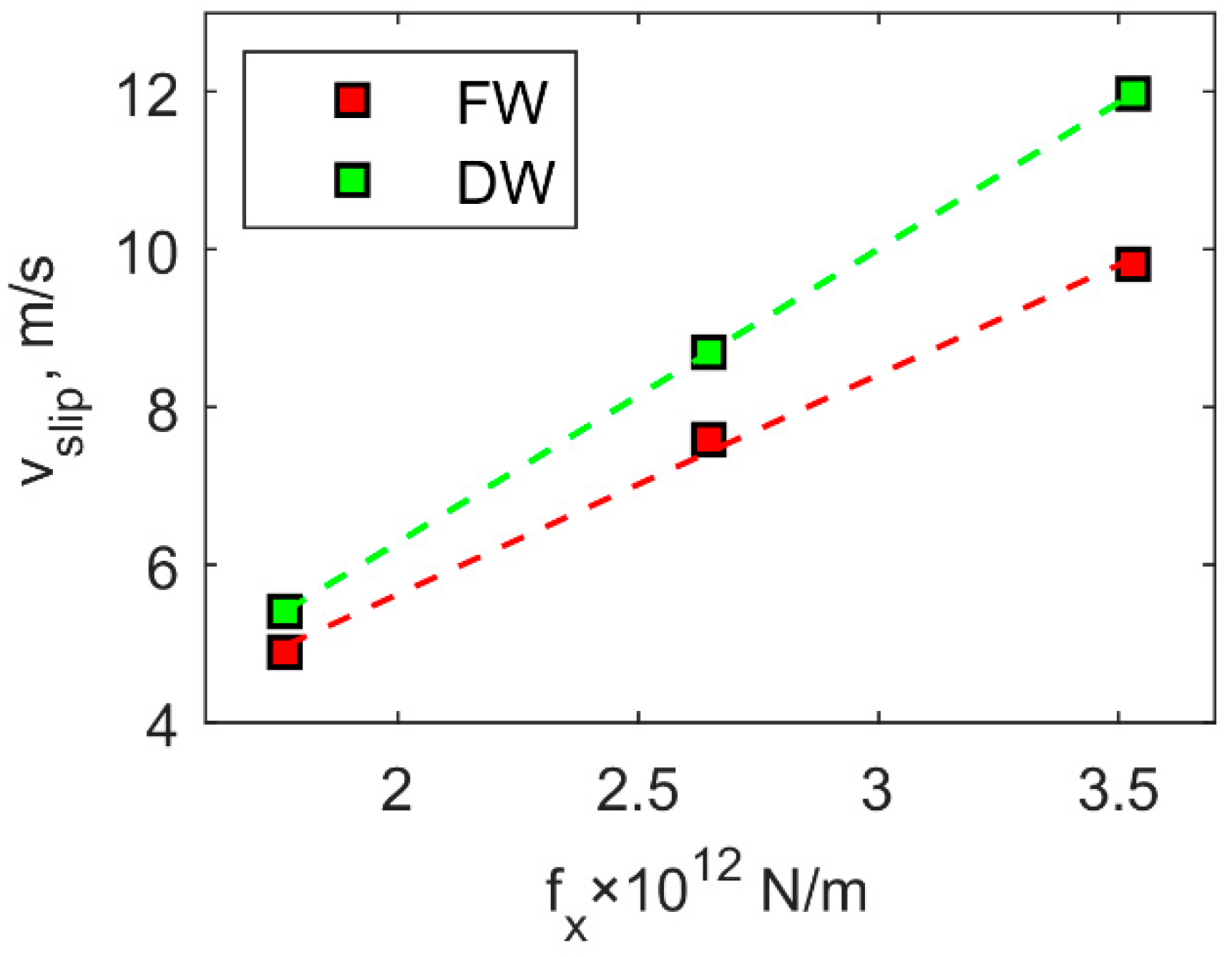
3.3. Flow Profiles and Slip Velocity

Water flow velocity profiles along the z-axis in FW and DW simulations at three different values of flow inducing force $f_x$ and comparison with the Navier–Stokes (NS) equation solutions for the water flow between two parallel plates are given in Figure 5. The simulation results show that the first layers of water molecules at the channel boundary travel along the x-axis with slip velocity $v_{slip}$. The slip velocity is expected as the Knudsen number of the simulated system is around 0.04, which corresponds to the slip flow regime satisfying $0.1>Kn>0.01$ [63]. Thus, the NS solutions were raised by the slip velocity $v_{slip}$ for each simulation case to directly compare simulation profiles with continuum solution:

$$v_x\left(z\right)=v_{x, NS}\left(z\right)+v_{slip}=-\frac{\rho }{2\mu }{f}_x\left(z^2-Hz\right)+v_{slip}.$$

(5)

Furthermore, the expression for NS mean flow velocity (without adding slip velocity) is:

$$v_{ave,NS}\left(f_x\right)=\frac{\rho }{12\mu }{f}_x{H}^2.$$

(6)

Here, $\rho =997 \mathrm{kg}/{\mathrm{m}}^3$ is the water density in the bulk region of the channel, and $H=44\mathsf{\AA }$ is the width of the channel. The viscosity $\mu =0.663 \mathrm{mPas}$ of SPC/E water model at 303 K temperature was taken from Markesteijn’s et al. [56] work, in which the authors evaluated the viscosity of various water models using the flow inducing force, the channel width, and, consequently, the flow velocity values similar to the ones used in present paper. The NS velocity profiles calculated with the SPC/E water viscosity value obtained by Markesteijn et al. [56] were in good agreement with the present simulation results (see Figure 5). Figure 5 also shows that the FW and DW temperature control strategies had no effect on shape of flow profile. We note that the slip velocity $v_{slip}$ for each case was found by fitting the simulation results with a parabolic fit and taking the average of the fit values at both boundaries of the channel, i.e., at the positions indicated by vertical dotted lines in Figure 5.

Figure 6 shows that the simulation mean flow velocity (excluding the slip velocity) to NS mean flow velocity ratio $v_{ave}/v_{ave, NS}$ is close to unity in both FW and DW simulations; however, the ratio values are slightly higher in DW simulations. The ratios with small deviations from unity demonstrate that flow in FW and DW simulations corresponds to NS solution for continuum flow in bulk region. Kucaba-Piętal et al. [26] also obtained parabolic velocity profiles for water flow inside copper and quartz channels. The water viscosity for TIP4P water at $300 \mathrm{K}$ was also evaluated to be $\mu =4.8 \mathrm{mPas}$ [56]. With such viscosity value, the ratios $v_{ave}/v_{ave, NS}$ in their copper channel simulations were 0.54 and 0.71 for channel widths $H=4.37\sigma$ and $H=9.35\sigma$, respectively. The disagreement with NS mean flow velocity could be explained by different water viscosity values at greater shear rates due to higher flow inducing force $f_x=2.85\times {10}^{14} \mathrm{N}/\mathrm{kg}$, which is more than one order higher than the force used in the present work.

It was previously shown that the slip velocity is influenced by the fluid molecular interactions with the solid walls; for example, Kucaba-Piętal et al. [26] showed that slip velocity for polar fluid (in their case water) is reduced when the electrostatic forces are introduced in channel walls while Zhang et al. [32] showed that slip velocity decreases when the solid–liquid interaction strength (described by the Lennard-Jones interaction parameter $\epsilon$) increases. On the other hand, the fluid interactions with solid walls in FW and DW simulations can also be interpreted as two different interaction types as the momentum exchange between fluid and solid atoms/molecules are considered in the DW simulations, which leads different collision mechanisms of water molecules with the copper atoms. Meanwhile, the fluid/solid momentum exchange is not considered in FW simulations. Consequently, the change of fluid behaviour at the interface could be expected in DW simulations in comparison with the FW simulations.

Indeed, Figure 7 shows that the slip velocities obtained in DW simulations are significantly greater than slip values in FW simulations with the same magnitude of flow inducing force $f_x$, and the difference in slip velocities increase with increasing value of $f_x$. The slip velocity in both FW and DW simulations is a linear function of $f_x$ in the investigated range of $f_x$, which can be written as

$$v_{slip}\left(f_x\right)=a{f}_x+b.$$

(7)

The coefficients $a$ and $b$ depend on the temperature control strategy and are listed in

Table 3. The slip velocity function (Equation (6)) coefficient values for FW and DW simulations.

Coeffiicients	FW Simulations	DW Simulations
$a\times {10}^{12}$$,{\mathrm{kgmN}}^{-1}{\mathrm{s}}^{-1}$	2.79	3.72
$b$$,{\mathrm{ms}}^{-1}$	0.060	−1.147

. The slip velocity to NS mean flow velocity ratio $v_{slip}/v_{ave, NS}$ was in the range from 1.14 to 1.40 in both FW and DW simulations, while the ratios in copper channel simulations by Kucaba-Piętal et al. [26] were 2.91 and 2.77 for channel widths $H=4.37\sigma$ and $H=9.35\sigma$, respectively. The difference in the $v_{ave}/v_{ave, NS}$ ratios could be caused by the different water models used in the simulations and the significantly different values of flow inducing force. However, the same order of the ratios in the present work and Kucaba-Piętal’s et al. [26] work indicate that the slip velocity for water flow inside copper channels are within the same order, regardless of the higher flow inducing force value. Furthermore, it shows that the slip velocity scales with both the flow inducing force and channel width. Similarly to present results for water, the LJ fluid simulations results by Priezjev [39] showed that slip length (which is closely related to slip velocity [28]) is also proportional to $f_x$, and the form of the proportionality depends of solid/wall interaction strength parameter ${\epsilon }_{sw}$: when the value of ${\epsilon }_{sw}$ is reduced, the slip length becomes non-linearly dependent on $f_x$, while with higher values of ${\epsilon }_{sw}$ the proportionality is linear. Furthermore, the change in fluid behaviour when the confinement atom dynamics are considered was also confirmed by Sam et al. [55] as they showed that the flow enhancement in CNTs (which is caused by the slip velocity) is significantly greater in CNTs with flexible tube walls compared to CNTs with rigid walls and thermostat applied directly to the fluid.

Let us note that the differences in slip velocity in our FW and DW simulations could also be influenced by the different simulation temperatures (see Table 2). However, the difference between slip velocities in FW and DW simulations is greater than could be expected from the 0.19 K difference in simulation temperatures when $f_x=1.77\times {10}^{12}\mathrm{N}/\mathrm{kg}$, which suggests that influence of temperature, in this case, is not significant. Therefore, the exact contributions of liquid/solid momentum exchange and slightly different simulation temperatures to the slip velocity could not be determined, and further research is needed.

On the contrary to our findings on water flow behaviour between two parallel solid plates, Zhang et al. [32] previously showed different behaviour for pressure-driven flows of LJ fluids. In their study, the authors investigated the influences of the strength of the solid-fluid coupling, the fluid temperature, and the density of the solid wall on the velocity slip at the fluid boundary. They showed that for LJ fluid, the factors influencing the slip velocity at the channel boundary also influenced the maximum flow velocity at the middle channel (when the slip velocity was subtracted from velocity profile), while our results for water showed that the flow behaviour of water in the channel does not depend on slip velocity, and is well described by continuum solution.

4. Conclusions

In the present paper, molecular dynamics simulations were performed to study the influence of two temperature control strategies on water flow behaviour inside planar nanochannel when the flow was induced by force acting on each water molecule in the channel. Two temperature control strategies were studied: (a) frozen wall simulations, in which the dynamics of confining wall atoms was not solved (frozen walls) and the thermostat was applied to the water, and (b) dynamic wall simulations, in which the dynamics of confining wall atoms was solved, and the thermostat was applied to walls while water was simulated in the microcanonical ensemble. The following conclusions can be drawn from the investigation results:

• the water temperature during steady flow state in simulations where the temperature is controlled through the channel walls might be slightly higher than the targeted simulation temperature due to the finite thermal conductivity in bulk water and liquid–solid interface and, consequently, this could change the temperature-dependent dynamic properties of water in the channel;
• the peaks in the water density profiles show the water layering effect near the channel walls, which is caused by correlated effects of long-range molecular attraction and short-range repulsion between copper and oxygen atoms. Furthermore, as the water cannot occupy the whole volume between solid walls, the channel boundaries are considered to be at density peak locations;
• the temperature control strategies considered in simulations had no effect on the shape of the water flow profile, and flow behaviour in the channel is well described by the Navier–Stokes equation solution with added slip velocity. Meanwhile, the slip velocity occurring at the boundaries of the channel is linearly dependent on the magnitude of flow inducing force in both frozen wall and dynamic wall simulations. However, the slip velocity is considerably greater in simulations, when the wall dynamics are solved in contrast to the frozen wall simulations, which is caused by the different collision mechanisms of water molecules with the copper atoms at the interface when the exchange of momentum is considered and the slightly different simulation temperatures.

References

1. Abgrall, P.; Nguyen, N.T. Nanofluidic devices and their applications. Anal. Chem. 2008, 80, 2326–2341. [Google Scholar] [CrossRef]
2. Murshed, S.; de Castro, N. A critical review of traditional and emerging techniques and fluids for electronics cooling. Renew. Sustain. Energy Rev. 2017, 78, 821–833. [Google Scholar] [CrossRef]
3. Wang, C.; Kazoe, Y.; Morikawa, K.; Shimizu, H.; Pihosh, Y.; Mawatari, K.; Kitamori, T. Micro heat pipe device utilizing extended nanofluidics. RSC Adv. 2017, 7, 50591–50597. [Google Scholar] [CrossRef] [Green Version]
4. Hu, C.; Wang, R.; Yang, P.; Ling, W.; Zeng, M.; Qian, J.; Wang, Q. Numerical Investigation on Two-Phase Flow Heat Transfer Parallel Channels. Energies 2021, 14, 4408. [Google Scholar] [CrossRef]
5. Liu, B.; Wu, R.; Baimova, J.A.; Wu, H.; Law, A.W.K.; Dmitriev, S.V.; Zhou, K. Molecular dynamics study of pressure-driven water transport through graphene bilayers. Phys. Chem. Chem. Phys. 2016, 18, 1886–1896. [Google Scholar] [CrossRef]
6. Weerakoon-Ratnayake, K.M.; O’Neil, C.E.; Uba, F.I.; Soper, S.A. Thermoplastic nanofluidic devices for biomedical applications. Lab. Chip 2017, 17, 362–381. [Google Scholar] [CrossRef] [PubMed] [Green Version]
7. Duan, C.; Wang, W.; Xie, Q. Review Article: Fabrication of Nanofluidic Devices. Biomicrofluidics 2013, 7, 026501. [Google Scholar] [CrossRef] [PubMed] [Green Version]
8. Bocquet, L.; Charlaix, E. Nanofluidics, from bulk to interfaces. Chem. Soc. Rev. 2010, 39, 1073–1095. [Google Scholar] [CrossRef] [Green Version]
9. Karniadakis, G.; Beskok, A.; Aluru, N. Microflows and Nanoflows: Fundamentals and Simulation; Springer Science: New York, NY, USA, 2005; ISBN 0387971734. [Google Scholar]
10. Vo, T.Q.; Kim, B. Transport phenomena of water in molecular fluidic channels. Sci. Rep. 2016, 6, 1–8. [Google Scholar] [CrossRef] [PubMed] [Green Version]
11. Hansen, J.S.; Dyre, J.C.; Daivis, P.; Todd, B.D.; Bruus, H. Continuum Nanofluidics. Langmuir 2015, 31, 13275–13289. [Google Scholar] [CrossRef] [Green Version]
12. Tuckerman, M.E.; Martyna, G.J. Understanding Modern Molecular Dynamics: Techniques and Applications. J. Phys. Chem. B 2000, 104, 159–178. [Google Scholar] [CrossRef]
13. Noorian, H.; Toghraie, D.; Azimian, A.R. The effects of surface roughness geometry of flow undergoing Poiseuille flow by molecular dynamics simulation. Heat Mass Transf. Stoffuebertragung 2014, 50, 95–104. [Google Scholar] [CrossRef]
14. Noorian, H.; Toghraie, D.; Azimian, A.R. Molecular dynamics simulation of Poiseuille flow in a rough nano channel with checker surface roughnesses geometry. Heat Mass Transf. Stoffuebertragung 2014, 50, 105–113. [Google Scholar] [CrossRef]
15. Yan, S.R.; Toghraie, D.; Hekmatifar, M.; Miansari, M.; Rostami, S. Molecular dynamics simulation of Water-Copper nanofluid flow in a three-dimensional nanochannel with different types of surface roughness geometry for energy economic management. J. Mol. Liq. 2020, 311, 113222. [Google Scholar] [CrossRef]
16. Alipour, P.; Toghraie, D.; Karimipour, A.; Hajian, M. Modeling different structures in perturbed Poiseuille flow in a nanochannel by using of molecular dynamics simulation: Study the equilibrium. Phys. A Stat. Mech. Its Appl. 2019, 515, 13–30. [Google Scholar] [CrossRef]
17. Alipour, P.; Toghraie, D.; Karimipour, A.; Hajian, M. Molecular dynamics simulation of fluid flow passing through a nanochannel: Effects of geometric shape of roughnesses. J. Mol. Liq. 2019, 275, 192–203. [Google Scholar] [CrossRef]
18. Lin, X.; Bao, F.B.; Gao, X.; Chen, J. Molecular dynamics simulation of nanoscale channel flows with rough wall using the virtual-wall model. J. Nanotechnol. 2018, 2018. [Google Scholar] [CrossRef] [Green Version]
19. Yang, S.C. Effects of surface roughness and interface wettability on nanoscale flow in a nanochannel. Microfluid. Nanofluid. 2006, 2, 501–511. [Google Scholar] [CrossRef]
20. Song, F.Q.; Wang, J.D. Investigation of influence of wettability on poiseuille flow via molecular dynamics simulation. J. Hydrodyn. 2010, 22, 513–517. [Google Scholar] [CrossRef]
21. Nagayama, G.; Cheng, P. Effects of interface wettability on microscale flow by molecular dynamics simulation. Int. J. Heat Mass Transf. 2004, 47, 501–513. [Google Scholar] [CrossRef]
22. Chen, W.; Foster, A.S.; Alava, M.J.; Laurson, L. Stick-slip control in nanoscale boundary lubrication by surface wettability. Phys. Rev. Lett. 2015, 114, 1–5. [Google Scholar] [CrossRef] [PubMed] [Green Version]
23. Yao, S.; Wang, J.; Liu, X.; Jiao, Y. The effects of surface topography and non-uniform wettability on fluid flow and interface slip in rough nanochannel. J. Mol. Liq. 2020, 301, 112460. [Google Scholar] [CrossRef]
24. Chen, X.; Cao, G.; Han, A.; Punyamurtula, V.K.; Liu, L.; Culligan, P.J.; Kim, T.; Qiao, Y. Nanoscale fluid transport: Size and rate effects. Nano Lett. 2008, 8, 2988–2992. [Google Scholar] [CrossRef] [PubMed]
25. Calabrò, F. Modeling the effects of material chemistry on water flow enhancement in nanotube membranes. MRS Bull. 2017, 42, 289–293. [Google Scholar] [CrossRef]
26. Kucaba-Pietal, A.; Walenta, Z.; Peradzyński, Z. Molecular dynamics computer simulation of water flows in nanochannels. Bull. Polish Acad. Sci. Tech. Sci. 2009, 57, 55–61. [Google Scholar] [CrossRef] [Green Version]
27. Soong, C.Y.; Yen, T.H.; Tzeng, P.Y. Molecular dynamics simulation of nanochannel flows with effects of wall lattice-fluid interactions. Phys. Rev. E 2007, 76, 1–14. [Google Scholar] [CrossRef] [PubMed]
28. Morciano, M.; Fasano, M.; Nold, A.; Braga, C.; Yatsyshin, P.; Sibley, D.N.; Goddard, B.D.; Chiavazzo, E.; Asinari, P.; Kalliadasis, S. Nonequilibrium molecular dynamics simulations of nanoconfined fluids at solid-liquid interfaces. J. Chem. Phys. 2017, 146. [Google Scholar] [CrossRef] [PubMed] [Green Version]
29. Ghorbanian, J.; Beskok, A. Scale effects in nanochannel liquid flows. Microfluid. Nanofluid. 2016, 20, 1–11. [Google Scholar] [CrossRef]
30. Yen, T.H. Effects of wettability and interfacial nanobubbles on flow through structured nanochannels: An investigation of molecular dynamics. Mol. Phys. 2015, 113, 3783–3795. [Google Scholar] [CrossRef]
31. Rezaei, M.; Azimian, A.R.; Semiromi, D.T. The surface charge density effect on the electro-osmotic flow in a nanochannel: A molecular dynamics study. Heat Mass Transf. Stoffuebertragung 2015, 51, 661–670. [Google Scholar] [CrossRef]
32. Zhang, H.; Zhang, Z.; Ye, H. Molecular dynamics-based prediction of boundary slip of fluids in nanochannels. Microfluid. Nanofluid. 2012, 12, 107–115. [Google Scholar] [CrossRef]
33. Marable, D.C.; Shin, S.; Yousefzadi Nobakht, A. Investigation into the microscopic mechanisms influencing convective heat transfer of water flow in graphene nanochannels. Int. J. Heat Mass Transf. 2017, 109, 28–39. [Google Scholar] [CrossRef] [Green Version]
34. Wu, K.; Chen, Z.; Li, J.; Li, X.; Xu, J.; Dong, X. Wettability effect on nanoconfined water flow. Proc. Natl. Acad. Sci. USA 2017, 114, 3358–3363. [Google Scholar] [CrossRef] [Green Version]
35. Shaat, M. Viscosity of Water Interfaces with Hydrophobic Nanopores: Application to Water Flow in Carbon Nanotubes. Langmuir 2017, 33, 12814–12819. [Google Scholar] [CrossRef]
36. Qin, X.; Yuan, Q.; Zhao, Y.; Xie, S.; Liu, Z. Measurement of the rate of water translocation through carbon nanotubes. Nano Lett. 2011, 11, 2173–2177. [Google Scholar] [CrossRef] [PubMed]
37. Zhang, Z.; Zhang, H.; Ye, H. Pressure-driven flow in parallel-plate nanochannels. Appl. Phys. Lett. 2009, 95, 10–13. [Google Scholar] [CrossRef]
38. Zhang, H.; Zhang, Z.; Zheng, Y.; Ye, H. Corrected second-order slip boundary condition for fluid flows in nanochannels. Phys. Rev. E 2010, 81, 1–6. [Google Scholar] [CrossRef] [PubMed]
39. Priezjev, N.V. Rate-dependent slip boundary conditions for simple fluids. Phys. Rev. E 2007, 75, 1–7. [Google Scholar] [CrossRef] [PubMed] [Green Version]
40. Suk, M.E.; Aluru, N.R. Modeling Water Flow Through Carbon Nanotube Membranes with Entrance/Exit Effects. Nanoscale Microscale Thermophys. Eng. 2017, 21, 247–262. [Google Scholar] [CrossRef]
41. Li, W.; Wang, W.; Zheng, X.; Dong, Z.; Yan, Y.; Zhang, J. Molecular dynamics simulations of water flow enhancement in carbon nanochannels. Comput. Mater. Sci. 2017, 136, 60–66. [Google Scholar] [CrossRef]
42. Falk, K.; Sedlmeier, F.; Joly, L.; Netz, R.R.; Bocquet, L. Molecular origin of fast water transport in carbon nanotube membranes: Superlubricity versus curvature dependent friction. Nano Lett. 2010, 10, 4067–4073. [Google Scholar] [CrossRef]
43. Bagheri Motlagh, M.; Kalteh, M. Simulating the convective heat transfer of nanofluid Poiseuille flow in a nanochannel by molecular dynamics method. Int. Commun. Heat Mass Transf. 2020, 111, 104478. [Google Scholar] [CrossRef]
44. Bagheri Motlagh, M.; Kalteh, M. Molecular dynamics simulation of nanofluid convective heat transfer in a nanochannel: Effect of nanoparticles shape, aggregation and wall roughness. J. Mol. Liq. 2020, 318. [Google Scholar] [CrossRef]
45. Jiang, Y.; Dehghan, S.; Karimipour, A.; Toghraie, D.; Li, Z.; Tlili, I. Effect of copper nanoparticles on thermal behavior of water flow in a zig-zag nanochannel using molecular dynamics simulation. Int. Commun. Heat Mass Transf. 2020, 116. [Google Scholar] [CrossRef]
46. Bantan, R.A.R.; Abu-Hamdeh, N.H.; Nusier, O.K.; Karimipour, A. The molecular dynamics study of aluminum nanoparticles effect on the atomic behavior of argon atoms inside zigzag nanochannel. J. Mol. Liq. 2021, 331. [Google Scholar] [CrossRef]
47. Asgari, A.; Nguyen, Q.; Karimipour, A.; Bach, Q.V.; Hekmatifar, M.; Sabetvand, R. Investigation of additives nanoparticles and sphere barriers effects on the fluid flow inside a nanochannel impressed by an extrinsic electric field: A molecular dynamics simulation. J. Mol. Liq. 2020, 318. [Google Scholar] [CrossRef]
48. Zhang, Z.Q.; Yuan, L.S.; Liu, Z.; Cheng, G.G.; Ye, H.F.; Ding, J.N. Flow behaviors of nanofluids in parallel-plate nanochannels influenced by the dynamics of nanoparticles. Comput. Mater. Sci. 2018, 145, 184–190. [Google Scholar] [CrossRef]
49. Philippe, H. Hünenberger Thermostat Algorithms for Molecular Dynamics Simulations. In Advanced Computer Simulation Approaches for Soft Matter Sciences I; Springer: Berlin, Germany, 2005. [Google Scholar]
50. Yong, X.; Zhang, L.T. Thermostats and thermostat strategies for molecular dynamics simulations of nanofluidics. J. Chem. Phys. 2013, 138. [Google Scholar] [CrossRef]
51. Basconi, J.E.; Shirts, M.R. Effects of temperature control algorithms on transport properties and kinetics in molecular dynamics simulations. J. Chem. Theory Comput. 2013, 9, 2887–2899. [Google Scholar] [CrossRef] [PubMed]
52. Kim, B.H.; Beskok, A.; Cagin, T. Thermal interactions in nanoscale fluid flow: Molecular dynamics simulations with solid-liquid interfaces. Microfluid. Nanofluid. 2008, 5, 551–559. [Google Scholar] [CrossRef]
53. Bernardi, S.; Todd, B.D.; Searles, D.J. Thermostating highly confined fluids. J. Chem. Phys. 2010, 132. [Google Scholar] [CrossRef] [Green Version]
54. Thomas, M.; Corry, B. Thermostat choice significantly influences water flow rates in molecular dynamics studies of carbon nanotubes. Microfluid. Nanofluid. 2015, 18, 41–47. [Google Scholar] [CrossRef]
55. Sam, A.; Kannam, S.K.; Hartkamp, R.; Sathian, S.P. Water flow in carbon nanotubes: The effect of tube flexibility and thermostat. J. Chem. Phys. 2017, 146. [Google Scholar] [CrossRef] [PubMed] [Green Version]
56. Markesteijn, A.P.; Hartkamp, R.; Luding, S.; Westerweel, J. A comparison of the value of viscosity for several water models using Poiseuille flow in a nano-channel. J. Chem. Phys. 2012, 136, 1–8. [Google Scholar] [CrossRef] [Green Version]
57. Berendsen, H.J.C.; Grigera, J.R.; Straatsma, T.P. The missing term in effective pair potentials. J. Phys. Chem. 1987, 91, 6269–6271. [Google Scholar] [CrossRef]
58. Skarbalius, G.; Džiugys, A.; Misiulis, E.; Navakas, R. Molecular dynamics study on water evaporation/condensation parameters. Microfluid. Nanofluid. 2021, 25, 1–13. [Google Scholar] [CrossRef]
59. Etesami, S.A.; Asadi, E. Molecular dynamics for near melting temperatures simulations of metals using modified embedded-atom method. J. Phys. Chem. Solids 2018, 112, 61–72. [Google Scholar] [CrossRef]
60. Plimpton, S. Fast Parallel Algorithms for Short-Range Molecular Dynamics. J. Comput. Phys. 1995, 117, 1–42. [Google Scholar] [CrossRef] [Green Version]
61. Maknickas, A.; Skarbalius, G.; Dziugys, A.; Misiulis, E. Nano-scale water Poiseuille flow: MD computational experiment. AIP Conf. Proc. 2020, 2239. [Google Scholar] [CrossRef]
62. Wang, S.; Javadpour, F.; Feng, Q. Fast mass transport of oil and supercritical carbon dioxide through organic nanopores in shale. Fuel 2016, 181. [Google Scholar] [CrossRef]
63. Abramovich, G.N. Applied Gas Dynamics, 3rd ed.; Ft. Belvoir Defense Technical Information Center: Fort Belvoir, VA, USA, 1973.
Figure 1. Visualisation of the simulated system.
Energies 14 06843 g001
Figure 2. The water flow in planar nanochannel temperature control strategies considered in MD simulations: (a) frozen wall (FW) simulations, in which the thermostat was applied directly to the flowing water, and copper wall atoms were frozen, and (b) dynamic wall (DW) simulations, in which the dynamics of copper atoms were solved, and the thermostat was applied only to copper walls.
Energies 14 06843 g002
Figure 3. Water temperature–time evolution in FW and DW simulations when the force inducing the flow was f x = 3.53 × 10 12   N / kg . Horizontal dotted line displays the average temperature of the copper in simulation with dynamic walls, while two vertical dotted lines is used as markers to separate the simulation stages.
Energies 14 06843 g003
Figure 4. Water density profile along the z-axis in FW and DW simulations when the force inducing the flow is   f x = 3.53 × 10 12   N / kg . Vertical dotted lines indicate σ C u O distances from the atomistic planes of the walls, which are in contact with water.
Energies 14 06843 g004
Figure 5. Water velocity profiles along the z-axis in (a) FW simulations and (b) DW simulations with varying values flow inducing force f x . The blue, red, and green markers represent simulation results with flow-inducing force values of 1.77 × 10 12 ,   2.65 × 10 12 ,   and   3.53 × 10 12   N / kg , respectively. Parabolic dotted lines represent NS solution (Equation (4)), while vertical dotted lines indicate σ C u O distances from the atomistic planes of the walls, which are in contact with water.
Energies 14 06843 g005
Figure 6. The simulation mean flow velocity (excluding the slip velocity) to NS mean flow velocity ratio as a function of the magnitude of flow inducing force in FW and DW simulations. The dotted line indicates the NS solution for the average flow velocity.
Energies 14 06843 g006
Figure 7. Slip velocity as a function of the magnitude of flow inducing force in FW and DW simulations.
Energies 14 06843 g007