A Case Study on the Water-Oil Interface of Shunbei Oilfield Based on Dynamic Data

Abstract

Shunbei Oilfield is characterized by substantial heterogeneity and a complex oil–water relationship. The water-oil interface is dynamically changing, and it is a crucial parameter for reserve calculation and evaluation. The main purpose is to analyze the effect of fluid flow in multi-scale media on the water-oil interface. It is well known that the fracture-cavity reservoirs have well-developed fractures and karst caves, and their distribution is complex in Shunbei Oilfield. This paper presents a way to simplify the fracture-cavity system first, then uses a unit of oil wells as a system to study the water-oil interface, which avoids impact on the water-oil interface due to oil production. A detailed step by step procedure for solving the semi-analytical solution of water-oil interface in a fracture-cavity reservoir by using an explicit algorithm and a successive steady-state method is presented. The solution can be used to investigate water-oil interface behavior. In this paper, we validated this method with the actual data for a relatively similar actual reservoir. Sensitivity analyses about the effects of the main parameters including production rates, cave volume and initial oil–water volume ratio on interfacial migration velocity are also presented in detail. The water breaking time of oil wells is fully investigated. The water-oil interface movement chart under different development conditions is established to predict the water-oil interface in the late stage of oil well production and extend the waterless developing period. Being based on this chart, a water breakthrough warning can be realized, and oil recovery can be improved. The findings of the research have led to the conclusion that the rising speed of water-oil interface is proportional to the production rate, on the contrary, it is inversely proportional to cave volume and initial oil–water volume ratio. As well production goes on, the water-oil interface rises at different rates. After the well is put into production for one year, the water-oil interface rises by 16.38%, 12.56% and 4.24% according to the condition that production rate is 10%, the initial oil–water volume ratio is 0.7, and the cave volume is 100 × 10⁴ m³. This method is not only suitable for any period and any well type in the development of Shunbei Oilfield; it also has the function of calculating the real-time water-oil interface of a single well and multi-wells. This new method has the characteristics of easy calculation and high accuracy. The method in this paper can be further developed as it has great applicability in fracture-cavity reservoirs.

1. Introduction

Due to the gravity differentiation and adjustment in a reservoir, oil occupies the high part of the reservoir [1], and water is located at the bottom or edge of the reservoir. The contact surface between oil and water is called water-oil interface (WOC). It is of great practical significance for reservoir development to accurately understand the depth of WOC in different oil wells and formulate reasonable development countermeasures [2].

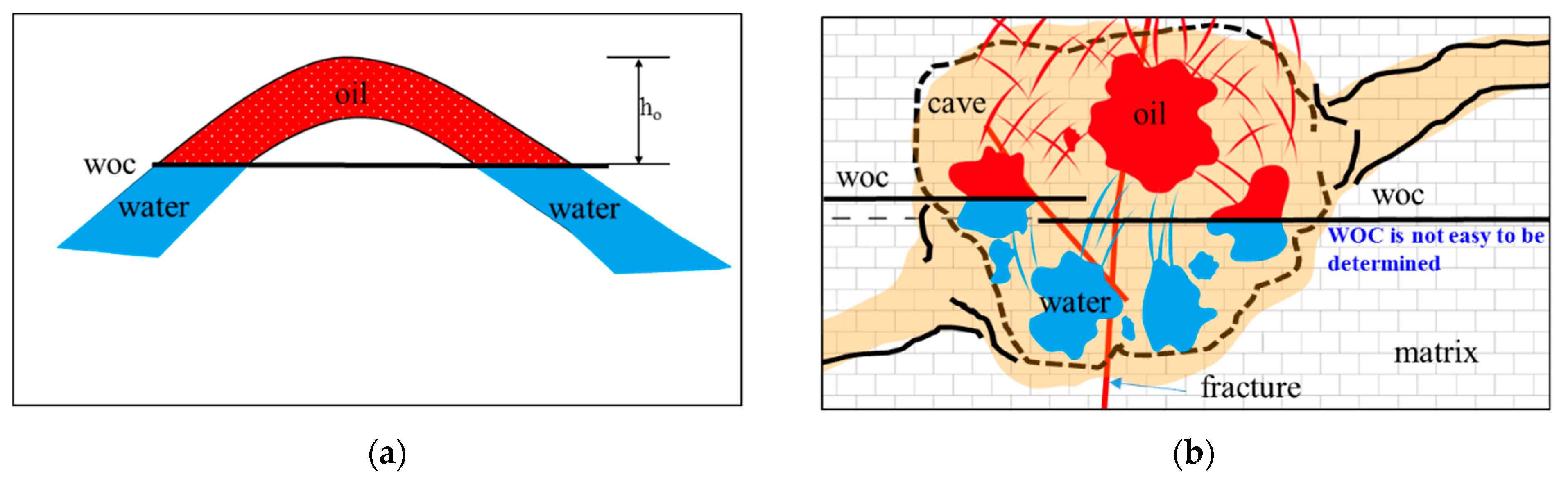
For the Shunbei Oilfield, the early oil and gas charging mainly migrated upward along the fault and then adjusted laterally [3]. Due to the unique storage space of fractured-cavity reservoirs, oil and gas are generally concentrated in caves, fractures or dissolved pores. During the development of fractured-cavity reservoirs, the oil–water relationship is more complicated. The speed of gravity differentiation between matrix or karst caves is different [4]. Traditional sandstone reservoirs have a unified WOC, but the fractured-cavity reservoir does not have a unified WOC, as shown in Figure 1.

At present, the calculation of water-oil interface in fractured-vuggy reservoirs is mainly based on the original water-oil interface and the dynamic water-oil interface during development.

1.1. Static WOC

The height of WOC is usually calculated by analyzing the force of WOC based on the basic parameters in the fracture-hole and combining with formation pressure, capillary force and gravity.

Gray used natural potential curve to identify WOC [5]. Through judging the fluid’s quality in the reservoir according to the characteristics of the longitudinal variation of the abnormal amplitude of the spontaneous potential, the WOC is obtained. Huang and Lian et al. used the neutron-gamma logging curve and resistivity method logging curve to identify the WOC through different physical parameters of oil and water [6,7]. Based on NMR logging technology, Luo et al. established the oil phase, water phase and T2 value relationship functions by extracting the characteristic parameters of the nuclear magnetic resonance T2 spectrum of the core test, and indirectly obtained the WOC [8].

Chen et al. [9] selected the pressure gradient method and the single well pressure gradient method to determine the original WOC in the study area. The pressure gradient method calculates the height of the WOC based on the different slopes reflected by different fluids in the pressure gradient map. The intersection of the pressure gradient lines is the static WOC. The single-well pressure gradient method is suitable for that when the number of wells is small and the pressure gradient data cannot be obtained; the original reservoir pressure and fluid density data of a single well can be used to calculate the WOC. There are some other pressure related methods, as shown in

Table 1. Some WOC calculation formulas.

Method	Formula	Limitation of the Utilization
Static pressure test method	$D_{woc}=\frac{\left(0.01{\rho }_w{D}_w-{\rho }_w\right)-\left(0.01{\rho }_o{D}_o-{\rho }_o\right)}{0.01\left({\rho }_w-{\rho }_o\right)}$	The production well needs to penetrate the entire reservoir [12].
Well test method	$D_{woc}=D_o+\frac{\left(p_i-p_w\right)}{0.01\left({\rho }_w-{\rho }_o\right)}$	The hydrostatic pressure at the WOC is challenging to determine [13].
Residual pressure method	$D_{woc}=D-\alpha ∆p$	It is not suitable for reservoirs with minor oil–water density differences [14].
Pressure formula method	$D_{woc}=D_o+\frac{p_i-0.01{\rho }_w{D}_o}{0.01\left({\rho }_w-{\rho }_o\right)}$	It is only suitable for reservoirs with bottom water or edge water [15].
Saturation projection method	$D_{woc}=\frac{hlog{s}_{wi-}{h}_{wi}log{s}_w}{log{s}_{wi-}log{s}_w}$	It needs to measure saturation, which is difficult in fracture-cavity reservoirs [16].
Core Test Method	$D_{woc}=h_o+\frac{\sigma }{4.9r_{min}\left({\rho }_w-{\rho }_o\right)}$	The minimum throat radius needs to be measured, which is difficult for fracture-cavity reservoirs [17].

Where ${\rho }_o$ is the density of underground crude oil, g/cm³; ${\rho }_w$ is the density of formation water, g/cm³; h is the height of the reservoir above the free water surface of the reservoir, m; σ is oil–water interfacial tension under formation conditions, mN/m; p_i, p_w is the original formation pressure and the static water column pressure when the depth is D₀; S_wi is the irreducible water saturation of the oil layer; h_wi is the corresponding depth when the irreducible water saturation of the oil layer is S_wi; S_w is the water saturation corresponding to that and the depth of the oil layer is h.

Luo et al. [10] used the mercury pressure curve of the original development well and used a variety of nonlinear equation methods to regress and fit the functional relationship between fluid saturation and capillary pressure. Then they combined with conventional logging interpretation results and fitted the function of the best free surface depth. Finally, they used the relationship between the free water surface and the WOC to determine the depth of the WOC.

Qu [11] derives the WOC calculation formula based on the equilibrium equation of the bending liquid surface force in the fractures and karst caves, combined with the Laplace equation.

1.2. Dynamic WOC

The key point of determining the dynamic WOC in the development of fractured-cavity reservoirs is how to accurately simulate the oil–water flow in fractured-cavity reservoirs, and predict the WOC in real time in combination with the production performance or test data (well test, pressure measurement, etc.) of fractured-cavity reservoirs. At present, there are three main types of flow simulation in fractured-cavity reservoirs.

Multi-media method: Most scholars regard fracture, cavity and matrix as different media, and use a triple or multi-media equivalent continuous model to simulate the flow and well test analysis of fractured-cavity reservoirs. Karst caves are regarded as zero dimensional reservoirs and supply fractures in the form of quasi steady or unsteady channeling flow [18,19]. The flow in the cave is a seepage process, and the cave and fracture are equivalent to continuous media. However, at present, the multi-media method is mainly used to analyze productivity and well test interpretation, and there is little research on the location of WOC, mainly the improvement of pressure gradient method.

Discrete reservoir method: For the situation where the well is connected to the cave, some scholars assume that the pressure in the cave is equal to the flow pressure at the bottom of the well, giving the cave a storage constant [20,21]. In practice, the depth of a faulty karst reservoir is 6000 m. When the pressure gauge is not lowered into the cave, the flow of fluid in the cave into the wellbore is affected by gravity, friction and micro-compressibility, and the size of the wellbore is much smaller than that of the cave. The fluid velocity is quite different from the fluid velocity in the wellbore, and the pressure must also be different.

Free flow modeling method: Some scholars have adopted the free flow equation to establish the free flow of fluid in the karst cave, but they all adopt the numerical simulation method. The amount of simulation calculation for the connected flow of multiple karst caves driven by oil and water is too large [22], and cannot track the WOC efficiently and in real time.

1.3. Adaptability Discussion

Previous research has shown that there are many methods for determining the WOC for sandstone reservoirs, but few research results have been reported at this point concerning carbonate fracture-cavity oil reservoirs, especially the Shunbei Oilfield. This may be caused by the following factors.

(1)

For the Shunbei Oilfield, the fracture-cavity body of the reservoir is relatively developed. Its bedrock porosity is minor, and the permeability is low. It is a somewhat typical tight limestone with a very high carbon-oxygen ratio. The logging method has certain limitations when applied to fracture-cavity reservoirs, namely when the oil well has leaked (the well drills into karst cave, and the karst cave diameter is generally more than 0.5 m in Shunbei Oilfield), the logging operation cannot be performed at all. Therefore, using conventional logging methods, the WOC cannot be accurately detected. Even if the logging tool successfully runs downhole, only the original WOC can be measured. Due to the production of oil wells, the cost of logging the WOC is very high.

(2)

Due to the particularity of reservoir and permeability space in fracture-cavity reservoirs, there is almost no capillary pressure in Shunbei Oilfield. The flow is dominated by pipe flow instead of traditional seepage between caves or between dissolution holes. Therefore, the traditional theory of determining the WOC by capillary pressure is difficult to apply in the fracture-cavity reservoir.

(3)

The pressure gauge is lowered to the bottom of the fracture-cavity reservoir. According to incomplete statistics, the drilling encounter rate of karst caves in Shunbei Oilfield is more than 80%. It is difficult for the pressure gauge to stabilize, which affects the accuracy of pressure testing. According to development practice, the Shunbei Oilfield has edge water or bottom water, the water body has vital energy, and the oil–water relationship is complicated. It is difficult to obtain the static pressure data of the oil or water layer.

(4)

The reservoir of Shunbei Oilfield is a fractured body formed by two faults squeezing each other. On the one hand, drilling is highly likely to meet karst caves; on the other hand, the reservoir rocks are easily broken, which increases the difficulty of coring and makes it difficult to obtain a complete core. Even if a small portion of the core is removed, the core is vulnerable to breakage under pressure during laboratory core experiments, and accurate saturation and permeability data cannot be obtained.

Therefore, it is necessary to establish a new method to calculate the WOC.

2. Shunbei Oilfield Reservoir Characteristics

According to seismic data, the main fault in the Shunbei Oilfield is a steep fault with a large dip angle and a small fault distance. The dissolution mainly develops along the main fault [1]. On the plane, the distribution of the reservoirs is mainly controlled by the main faults and the secondary faults intersecting with them, and the degree of dissolution and fragmentation is relatively small. Each fault is distributed along the main fault and has a small width [21]. Inside the faults, fractures and dissolution pores are the main space for storing oil and gas; among the faults, the fractures connect the wells and adjacent caves [20].

The types of storage space in the Shunbei Oilfield can be divided into three types: fractures, pores and dissolved pores. The fractures in the Shunbei Oilfield are mainly unfilled to semi-filled, and the fillings are mostly calcite. There are many types of matrix pores in the study area, such as intercrystalline pores, intergranular pores, intercrystalline dissolved pores and intergranular dissolved pores, but they are not the main storage space. Shunbei Oilfield has a small degree of dissolution. They usually develop along the main fault and can be divided into worm-shaped karst caves and spherical karst caves.

The fluid flow in the reservoir mainly depends on the communication between fractures and caves [1]. Due to the random distribution of fractures and karst caves, it is generally impossible to form a good fracture-cave system, so the heterogeneity of fracture-cavity reservoirs is particularly strong [7]. The Shunbei Oilfield is a particular fracture-cavity reservoir and has some unique features [23]. In summary, it is mainly manifested in the following aspects:

(1)

A large number of unexposed karst fracture-cavity reservoirs are developed along the fault zone;

(2)

Reservoir storage space, storage type, fluid properties and distribution all show diversity and complexity. The horizontal heterogeneity is substantial, but the vertical connectivity is good. Comparing with caves, the matrix has no storage and permeability capabilities, and it requires hydraulic fracturing to communicate between the wellbore and the cave;

(3)

The reservoir is characterized by ultra-deep depth, ultra-high pressure and ultra-high temperature. The crude oil contains high hydrogen sulfide.

In the early stage of its development, the oil wells produce oil without water. Once the water breaks through the oil well, the water cut rises particularly quickly. How to stabilize the oil productivity and control the water cut has become a constraint key on developing the Shunbei Oilfield. If some technical methods can be used to determine the WOC in advance, then corresponding water control measures can be taken in a targeted and timely manner so the stable oil production in the Shunbei Oilfield can be ensured, and the oil recovery can be improved. The prerequisite for accurately judging the oil well’s water output’s location is determining the WOC. Therefore, studying the WOC is of great significance to the development of Shunbei Oilfield. In summary, there are mainly the following aspects:

(1)

For reserves estimation and reservoir evaluation, WOC is indispensable;

(2)

For layered, structural reservoirs, WOC is the direct basis for dividing their boundaries;

(3)

When the heterogeneity of reservoirs is extreme, the fluctuation of the WOC cannot be ignored.

3. Mathematical Model

The main purpose is to analyze the effect of fluid flow in multi-scale media on WOC. A detailed step by step procedure for solving the semi-analytical solution of WOC in a fracture-cavity reservoir by using explicit algorithm and successive steady-state method is presented. That is:

Step 1: Determine the fracture-cavity model based on the basic information of the oil well;

Step 2: The N–S equation considering the way of fluid flow (expressed by Reynolds number) is built, and the explicit step-by-step algorithm is introduced to obtain the flow velocity;

Step 3: The flow equation under the gravity differentiation is built, and the successive steady-state method is used to obtain the dynamic WOC.

The solution can be used to investigate WOC behavior. The water breaking time of oil wells is fully investigated. The advantage of the method is that it can reduce the amount of computation and compute efficiently.

3.1. Flow Model

For the convenience of research, the following assumptions were made in this paper:

(1)

The fracture-vuggy reservoir system is not regarded as a unified continuum model, but the entire system is considered to be composed of different flow units.

(2)

Since there are a large number of caves and fractures in fractured-vuggy reservoirs, the flow of liquid mainly occurs in them, so it is assumed that the seepage in the rock occurs in the fractures.

(3)

The karst cave is the main storage space, and the fluid is regarded as an incompressible viscous fluid, based on which the karst cave unit can be established.

(4)

Fractures are the main percolation channels which connect the caves and have a certain storage capacity. The flow in the fractures can be regarded as linear seepage, and the fracture unit can be established based on this.

(5)

The combination of the cave unit and the fracture unit can form the fracture-cavity unit. One-dimensional and two-dimensional flows are shown in Figure 2a and Figure 3a.

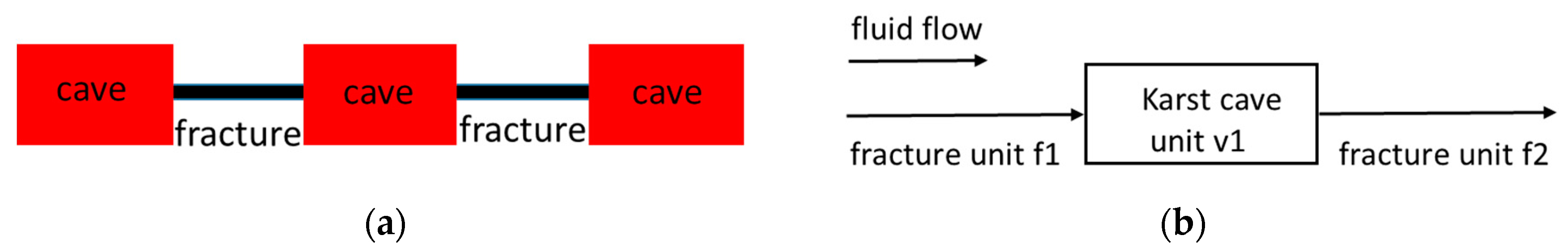
One-dimensional fracture-cavity system: The connection of the unit is relatively simple, basically the fracture unit and the cave unit are alternately connected, as shown in Figure 2b. There is always only one unit at each point along the flow direction, and the calculation only needs to start from the first unit according to the boundary conditions, then obtain the boundary conditions of the next unit and finally calculate each unit in turn along the flow direction.

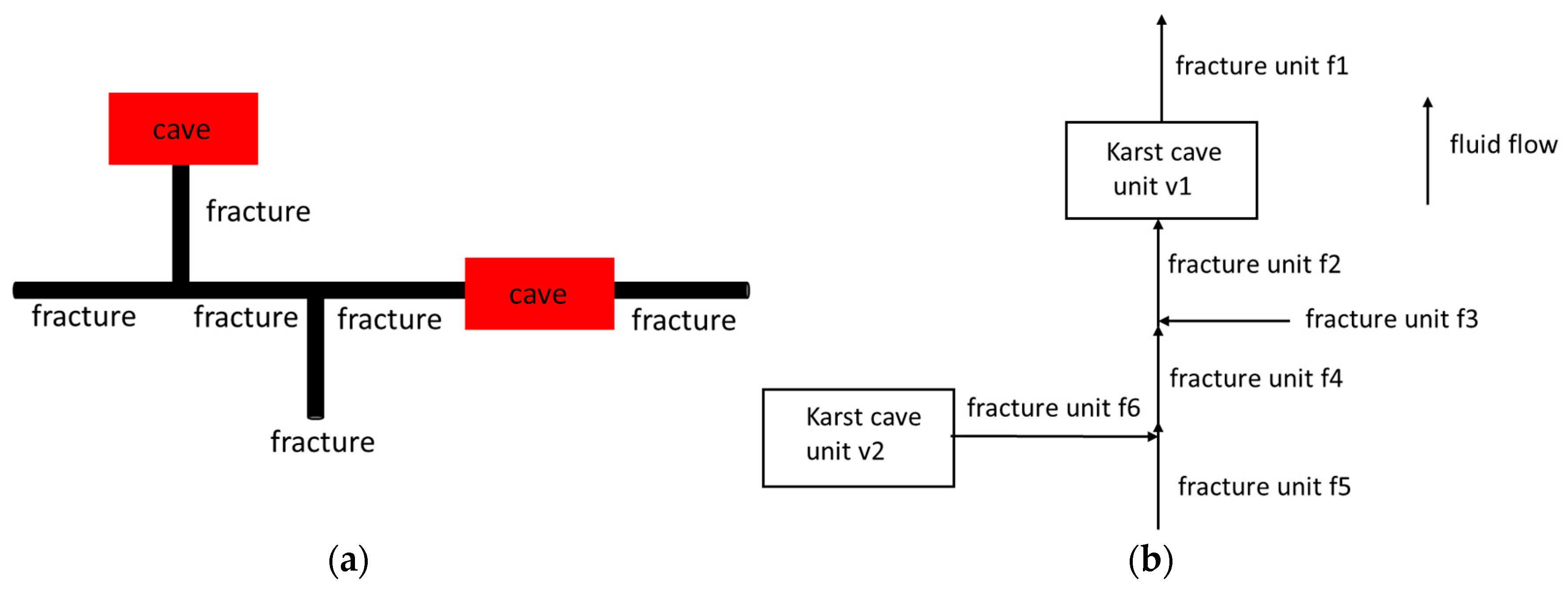
Two-dimensional fracture-cavity system: The connection of the units is in a mesh shape, as shown in Figure 3b, and the flow directions between different units are different. However, through analysis, it can be found that there is always a main flow direction in the plane (in reality, this direction is flowing to the well). The other flow directions are like the tributaries of the river, converging in the main flow direction. In this way, the main flow direction of the physical model can be established first, and then the connection of the entire mesh unit is simplified to the parallel connection of different units along the main flow direction by referring to the principle of pipeline flow. Given this, the two-dimensional fracture-cavity system model can be simplified to a one-dimensional fracture-cavity system model. The principle of dimensionality reduction is: Firstly, determine the main flow channel and flow direction according to the combined model of fractures and caves. Then, connect other fracture units that are not parallel with the fracture units in the main flow direction. The cave units that are not in the main flow direction are calculated according to their actual flow direction. The two-dimensional fracture-cavity system model in Figure 3 is simplified to a one-dimensional fracture-cavity system model, as shown in Figure 2.

This paper uses two karst-cavity units to illustrate the physical model of the fracture-cavity system. The model is mainly composed of two cave units and six fracture units. The model can be decomposed into two branch fluid flow channels and one main fluid flow channel. The first branch fluid flow channel mainly includes a cave unit v2 and a fracture unit f6. The second branch fluid flow channel mainly consists of a fracture unit f3. The main fluid flow channel consists of a cave unit v1and four fracture units—f1, f2, f4 and f5.

3.2. Mathematics Flow Model

3.2.1. Flow Velocity

Assuming that the cave unit is rectangular, the length and width are a and b, so the equivalent length converted into a square is L($L=\sqrt{\frac{ab}{\pi }}$). According to the continuity equation and motion equation of the fluid [15,24,25], the N–S equation is established as below:

$$\frac{\partial v}{\partial t}+v\frac{\partial v}{\partial r}=-\frac{\partial p}{\partial r}+\frac{1}{Re}\frac{{\partial }^{2}v}{\partial r^2}$$

(1)

where p is the pressure of the fluid; Re is the Reynolds number of the fracture, $Re=\frac{\rho w}{\mu }$; $w$ is the width of the fracture; $\rho$ is the density of the fluid; $\mu$ is the viscosity of the fluid; v is the flow velocity of the fluid.

Introduce an explicit step-by-step algorithm [25], and the Equation (1) can be rewritten as:

$$\frac{v^{n+1}-v^n}{∆t}+A\left(v^n\right)+\nabla p^{n+1}=\frac{1}{Re}{\nabla }^2{v}^n$$

(2)

where $A\left(v^n\right)$ is the fluid velocity correction item. It is defined as the projection of the intermediate velocity onto the velocity gradient, and it can be written as:$A\left(v^n\right)=v^{*}·v^n$.

Formula (2) is calculated within two steps, that is, the pressure effect is neglected in the first step, and the Formula (2) is simplified as

$$\frac{v^{*}-v^n}{∆t}+A\left(v^n\right)=\frac{1}{Re}{\nabla }^2{v}^n$$

(3)

where $v^{*}$ is the intermediate value of the flow rate.

In the second step, the pressure effect is revised as below:

$$\frac{v^{n+1}-v^{*}}{∆t}+\nabla p^{n+1}=0$$

(4)

Combining with the continuity equation:

$$\nabla v^{n+1}=0$$

(5)

The pressure calculation formula is shown as below:

$${\nabla }^2{p}^{n+1}=\frac{\nabla v^{*}}{∆t}$$

(6)

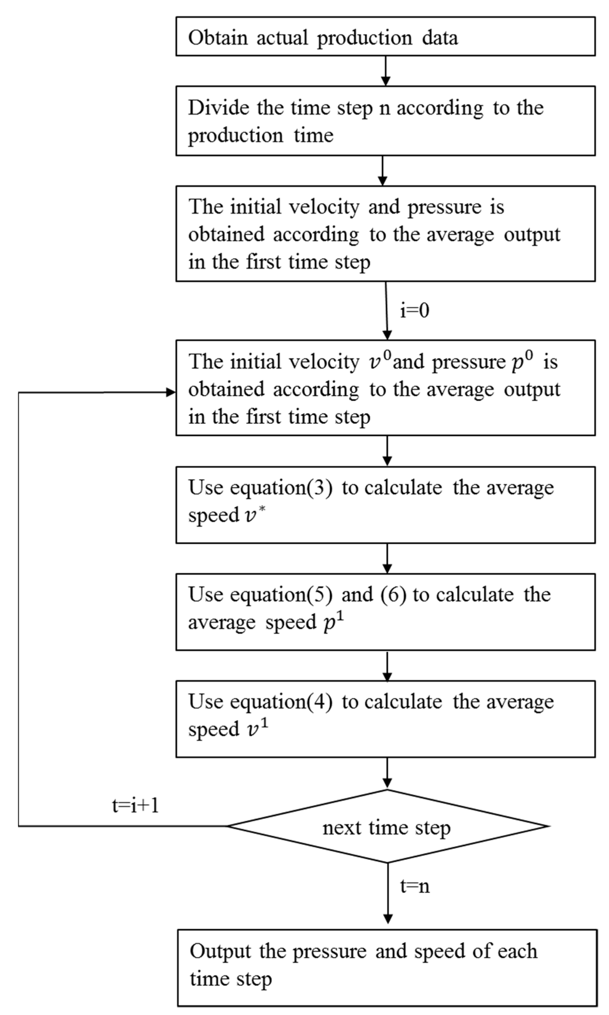
The steps for establishing the velocity field are shown in Figure 4.

3.2.2. Dynamic WOC

The time is equally divided into corresponding n time steps. It is considered that in each time step, the fracture-cavity unit is in a steady-state [26]. The successive steady-state method is used to solve the dynamic WOC variety.

Considering that the fluids in the fracture-cavity system are oil and water, both of which are viscous fluids, the velocity fields on the oil layer and water layer are different. However, when the fluid in the unfilled cavity tends to flow in a steady state, the velocity of oil phase and water phase at the WOC are the same. The flow equation and continuity equation under the gravity differentiation of oil and water are shown below [27].

$$v=-\frac{r^2}{8\mu }\frac{\partial [p-\left({\rho }_w-{\rho }_o\right)gz}{\partial z}$$

(7)

$$\frac{\partial v}{\partial z}=0$$

(8)

where: r is the radius of the unfilled cavity; $\mu$ is the viscosity of the fluid; ${\rho }_o$ and ${\rho }_w$ are the density of the oil phase and water phase, respectively; g is the acceleration of gravity.

Combining Equations (7) and (8), we can obtain:

$$\frac{{\partial }^{2}p}{\partial z^2}=0$$

(9)

The solution of Equation (9) is: $p=az+b$, so the pressure of the oil phase and water phase are shown as below (Liu, 2016, [14]).

$$\{\begin{array}{c}{p}_o=a_{o}z+b_o z>h_f\\ p_w=a_{w}z+b_w z<h_f\end{array}$$

(10)

where $p_o$ and $p_w$ are the pressure of the oil phase and water phase, respectively;$h_f$ is the WOC value.

At the WOC, the pressure and velocity of the oil phase and the water phase are equal, namely:

$$\{\begin{array}{c}{p}_o=p_w \\ v_w=-\frac{k_w}{{\mu }_w}\frac{\partial p_w}{\partial h_f}=v_o=-\frac{k_o}{{\mu }_o}\frac{\partial p_o}{\partial h_f} \end{array}$$

(11)

where $v_o$ and $v_w$ are the flow rates of the oil phase and water phase, respectively. $k_o$ and $k_w$ are the permeability of the oil phase and water phase, respectively. ${\mu }_o$ and ${\mu }_w$ are the viscosity of the oil phase and water phase, respectively.

Combining Equations (10) and (11), we can obtain:

$$a_w=\frac{\left(p_H-p_o\right)+\left({\rho }_w-{\rho }_o\right)g{h}_f}{MH+\left(1-M\right)h_f}$$

(12)

where: M is the fluidity ratio of water and oil; H is the height of unfilled cavity.

At the WOC, the oil-phase flow rate, the water-phase flow rate and the rising speed of the WOC are the same (Deng, et al., 2019, [1]), that is:

$$v_f=v_o=v_w={\lambda }_w\frac{\left(p_H-p_o\right)+\left({\rho }_w-{\rho }_o\right)g{h}_f}{MH+\left(1-M\right)h_f}$$

(13)

where ${\lambda }_w$ is the fluidity of the water; $v_f$ is the rising speed of the WOC.

Substitute the velocity field obtained in Section 2 into Equation (13). The WOC values at different time steps can be obtained.

4. Results and Discussions

4.1. Model Validation

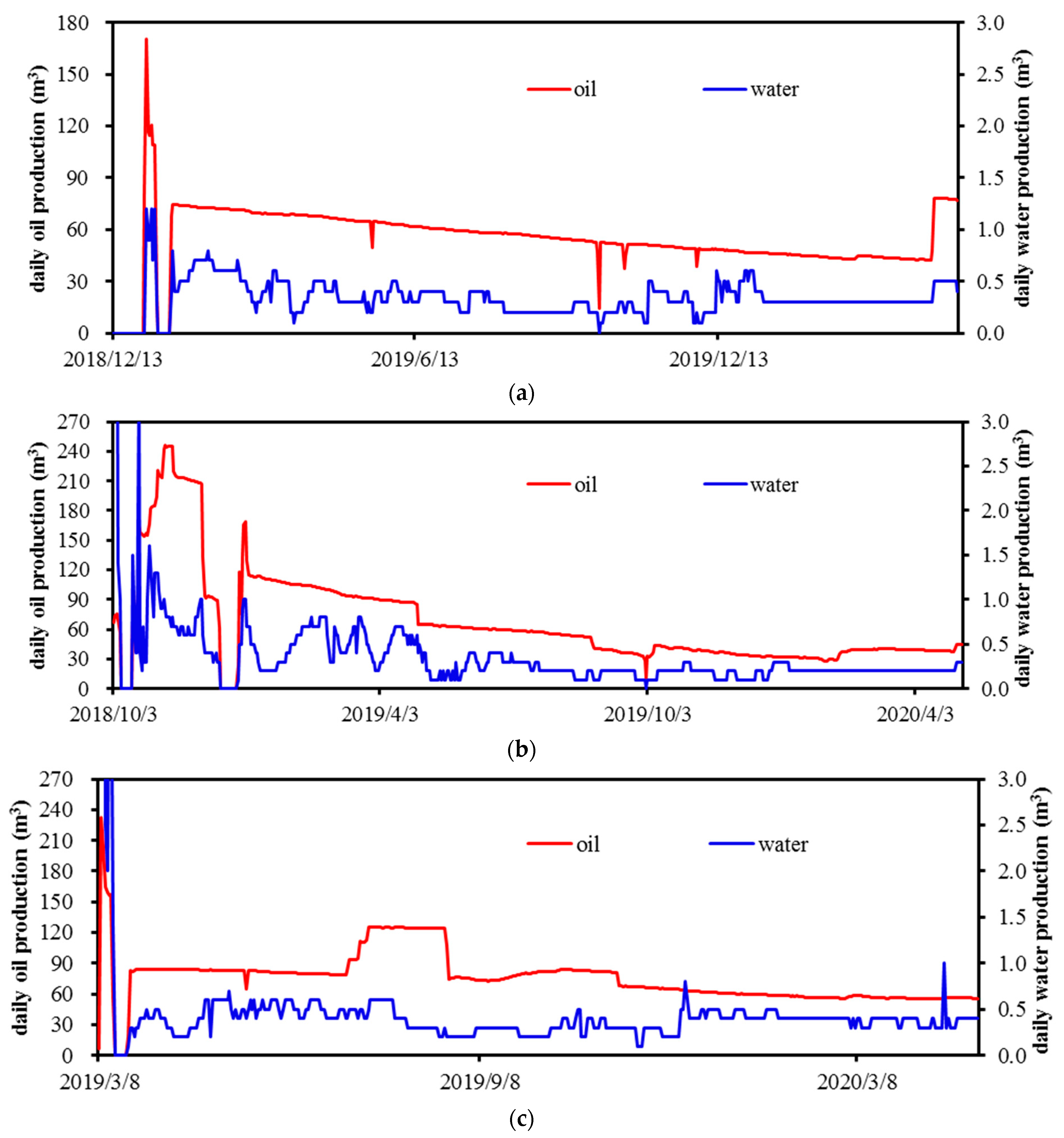
According to the actual production performance, the WOC was calculated and explained by taking wells A1, A2 and A3. Basic data for the three wells are shown in

Table 2. Basic data for the three wells, A1, A2 and A3.

Parameter	Value	Parameter	Value
original saturation pressure (MPa)	58	original reservoir pressure (MPa)	58
formation water density (g/cm3)	1	crude oil density (g/cm3)	0.87
formation water viscosity (mPa·s)	0.51	formation crude viscosity (mPa·s)	0.61
length of karst cave unit (m)	15	length of fracture element (m)	60
equivalent diameter of cave (m)	1.5	equivalent diameter of fracture (m)	0.01
filled cave permeability (mD)	300	fracture permeability (mD)	1000

and Figure 5.

(1) For the convenience of calculation, this paper only studies one year during the production period of these three wells (for A1, 2019.4.19–2020.4.19; for A2, 2019.4.26–2020.4.26; for A3, 2019.4.1–2020.4.1), the time step is set as 30 days, and the iteration is calculated 10 times. Firstly, according to the oil phase production and formation pressure after 30 days of production, the initial dimensionless velocity values of the three wells were given, namely:

$$\{\begin{array}{c}{v}_1^0=3.25 \left(A1\right)\\ v_2^0=4.11 \left(A2\right)\\ v_3^0=2.94 \left(A3\right)\end{array}$$

(14)

(2) Substitute the initial value of velocity obtained in step (1) into Equation (3), and the intermediate value of velocity under this time step can be obtained, namely:

$$\{\begin{array}{c}{v}_1^{*}=2.97 \left(A1\right)\\ v_2^{*}=3.89 \left(A2\right)\\ v_3^{*}=2.65 \left(A3\right)\end{array}$$

(15)

Meanwhile, by combining Equations (5) and (6), the initial pressure value is used to obtain the pressure value corresponding to the next time step, namely:

$$\{\begin{array}{c}{p}_1^1=24.96 \left(A1\right)\\ p_2^1=27.81 \left(A2\right)\\ p_3^1=21.45 \left(A3\right)\end{array}$$

(16)

(3) Substitute the median velocity and the pressure together into Equation (4) to obtain the next time step’s velocity, namely:

$$\{\begin{array}{c}{v}_1^1=2.69 \left(A1\right)\\ v_2^1=3.67 \left(A2\right)\\ v_3^1=2.36 \left(A3\right)\end{array}$$

(17)

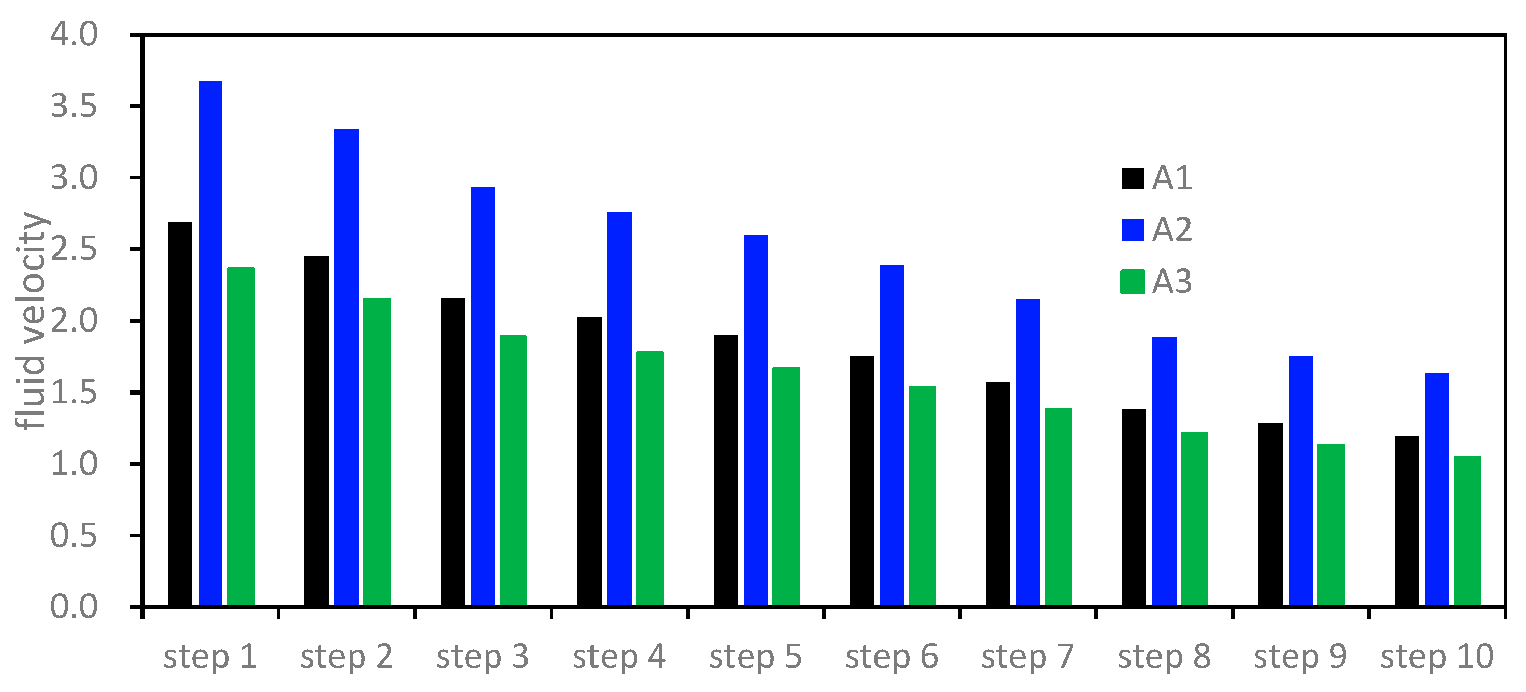
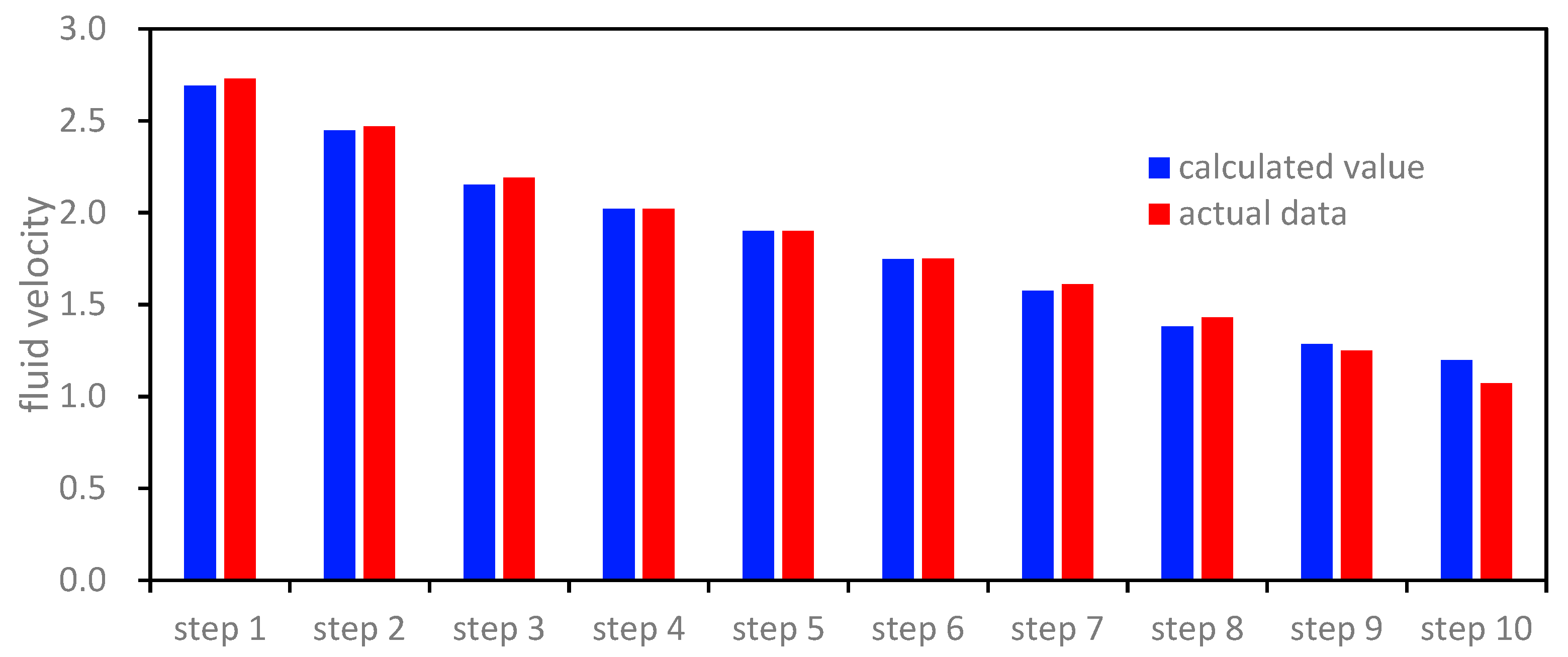
The velocity values and pressure values obtained in the above steps are successively substituted into Equations (3)–(6), and then the iterative method of establishing the velocity field is repeated to calculate the velocity field values at different times successively. The calculation results are shown in Figure 6. The actual oil phase velocity in each step calculated by dynamic data is compared with the computed results in this paper. The comparison results are shown in Figure 7. Figure 7 indicates that these two match very well, verifying the correctness of the method in this paper.

(4) The oil phase velocity value is substituted into Equation (13) and the WOC value under the production time is obtained.

$$\{\begin{array}{c}{h}_{woc1}=5678.87 \left(A1\right)\\ h_{woc2}=5531.92 \left(A2\right)\\ h_{woc3}=5472.64 \left(A3\right)\end{array}$$

(18)

The comparison results with the actual WOC monitoring data of this block are shown in

Table 3. Comparison results of actual WOC monitoring data.

Well Name	Calculating Value/m	Actual Data/m	Relative Error/%
A1	5678.87	5519.23	2.81
A2	5531.92	5562.71	0.55
A3	5472.64	5489.32	0.32

. Table 3 shows that the relative error is controlled within 5%, which belongs to the allowable error range, indicating that the calculation method in this paper is reasonable and scientific.

The the time step was set as 10 days, and the iteration was calculated 30 times. The corresponding calculation results are shown in

Table 4. Comparison results of actual WOC monitoring data.

Well Name	Calculating Value/m	Actual Data/m	Relative Error/%
A1	5507.18	5519.23	0.22
A2	5547.26	5562.71	0.28
A3	5484.91	5489.32	0.08

. The comparison of Table 3 and Table 4 shows that the shorter the time step is, the more iterations there are, and the more accurate the calculated WOC is.

Based on the calculation method in this paper, the WOC chart under different production conditions can be established, which is convenient for predicting the water-break time in the later producing period of oil, and provides guidance for water-break warning.

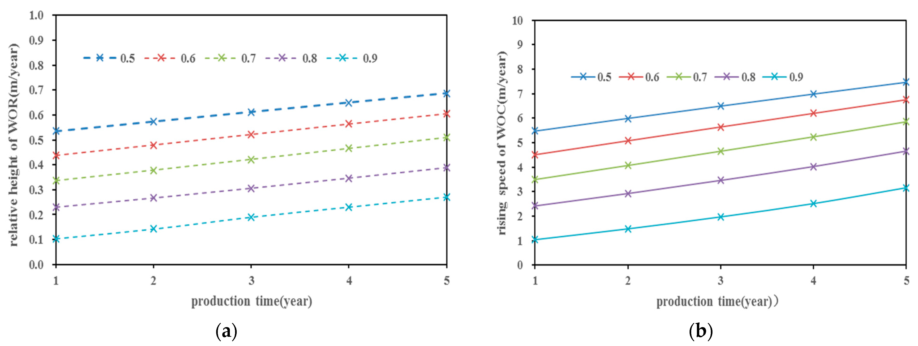
4.2. Sensitivity Analysis of Production Rate

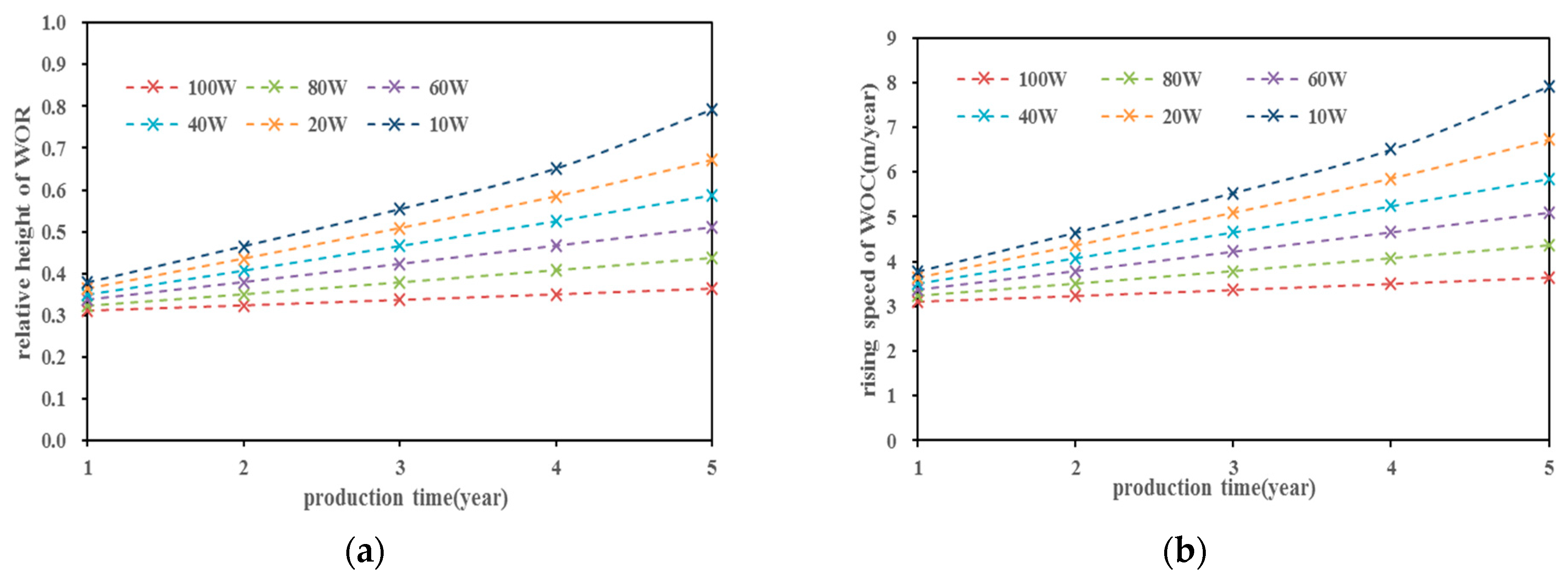
The relative height and rising speed of the WOC at different oil production rates are shown in Figure 8. As shown in Figure 8a, with the production time increasing, the WOC gradually rises. The relative height of WOC is directly proportional to the production rate. The greater the production rate is, the faster the WOC increases.

As shown in Figure 8b, the WOC’s rising speed is stable when the oil production rate (2.5%) is low. When the production rate (>5%) increases, the rising speed of the WOC gradually accelerates. There is an optimal speed between the WOC rising speed and the production rate, under which the change value of the WOC increasing speed is the least.

4.3. Sensitivity Analysis of Cave Volume

When the karst cave volume changes, the relative height of the WOC changes similarly, except for the data difference, as shown in Figure 9. As shown in Figure 9b, the WOC’s rising speed is stable when the cave volume (100 W) is large. When the cave volume (<80 W) decreases, the rising speed of the WOC gradually accelerates. The larger the cave volume is, the smaller the rising speed of the WOC is. Please note that W = × 10⁴ m³.

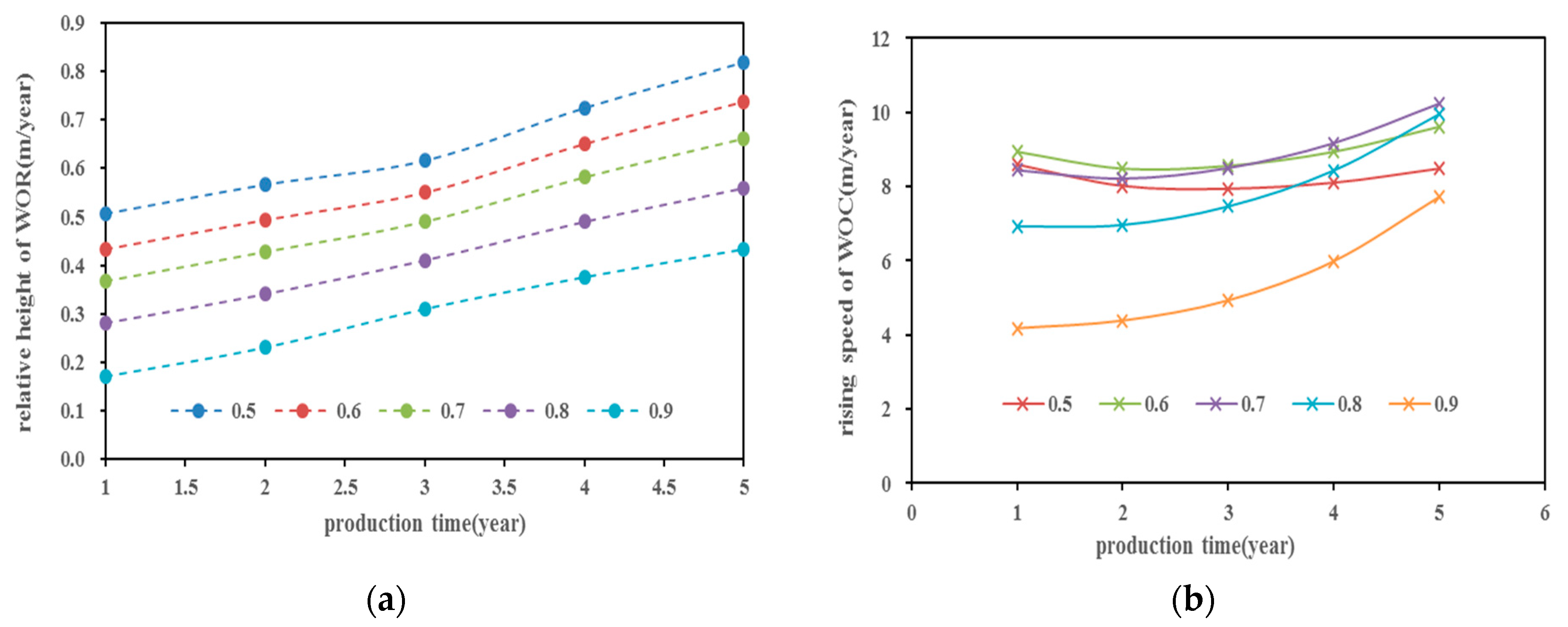
4.4. Sensitivity Analysis of Initial Oil–Water Volume Ratio

Production rates <10%: As shown in Figure 10, the relative height of the WOC presents a linear relationship with the production time (years). The changing trend of WOC has nothing to do with the initial oil–water volume ratio. The slope of all the curves is almost the same.

Production rates > 10%: As shown in Figure 11, when the initial oil–water volume ratio is less than 0.8, the rising speed of WOC decreases first and then increases slowly. When the initial oil–water ratio is greater than 0.8, the rising speed of WOC rises continuously. The trend of WOC rising speed is consistent under different oil production rates. When the oil production rate and the initial oil–water volume ratio are constant, the rising rate of the WOC increases with the increase of production time.

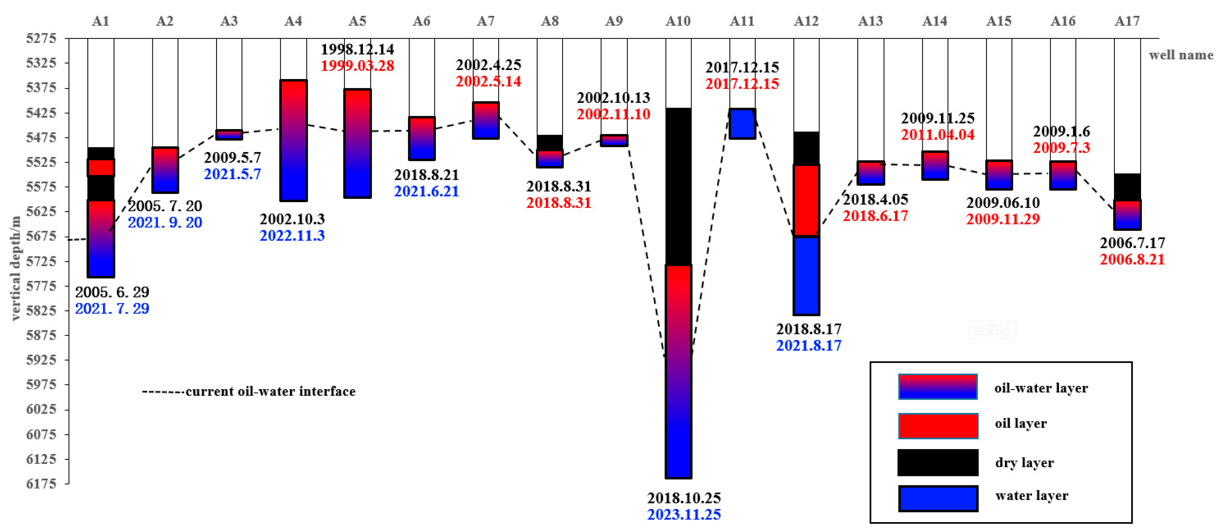
4.5. Field Application

According to the production characteristics under different conditions, we can predict the WOC in the later production period by comparing it with the WOC movement rule chart, as shown in Figure 12. Figure 12 shows that the water appearance time of the oil well is in good agreement with the time calculated by the model, which indirectly shows that the method in this paper is reasonable. This method can not only judge the position of the water-oil interface according to the test production of the new well, but it can also delay water invasion by adjusting production rate to ensure long-term stable production of the oil well, which helps to improve the recovery of a single well.

Please note that the time written in black indicates the beginning time of the production well. The time written in red indicates the water breakthrough time, while the time written in blue indicates the estimated water breakthrough time.

The biggest disadvantage of this approach is that it requires production data. Therefore, the initial water-oil interface of an unproduced well cannot be calculated. In view of this situation, the water-oil interface can be indirectly judged by analogy with the reservoir parameters of the well in production. The chart of reservoir physical property and water-oil interface can be established in the future to control the production rhythm of the whole oilfield and achieve the purpose of economic development.

5. Conclusions

This paper presents a new way to obtain the solution of WOC in a fracture-cavity reservoir. Compared with other conventional methods, the proposed method can calculate the WOC in real time from production data, and the calculation process is simple without measuring the permeability of oil and water phases.

As well production goes on, the WOC rises at different rates. After the well is put into production for one year, the WOC rises 16.38%, 12.56% and 4.24% according to the condition that production rate is 10%, the initial oil–water volume ratio is 0.7 and the cave volume is 100 × 10⁴ m³.

A key factor affecting the method in this paper is the time step. The shorter the time step is, the more iterations there are, and the more accurate the calculated WOC is. For well A1, when the time step is 30 days, the calculation error is 160m; when the time step is 10 days, the calculation error is 12.05 m.

References

- Deng, S.; Li, H.; Zhang, Z.; Zhang, J.; Yang, X. Structural characterization of intracratonic strike-slip faults in the central Tarim Basin. AAPG Bull. 2019, 103, 109–137. [Google Scholar] [CrossRef]
- McBride, J.H. Investigating the crustal structure of a strike-slip ‘step-over’zone along the Great Glen Fault. Tectonics 1994, 13, 1150–1160. [Google Scholar] [CrossRef]
- McBride, J.H. Structure of a continental strike-slip-fault from deep seismicre-flection—Walls Boundary Fault, Northern British Caledonides. J. Ofgeophys. Res.—Solid Earth 1994, 13, 2398–2405. [Google Scholar]
- Schulman, J.H. The Oil/Water Interface. Nature 1941, 147, 197–200. [Google Scholar] [CrossRef]
- Gray, W.J.; Willmon, G.J. WOC Measurements in Bottom Water Drive Pools. J. Can. Pet. Technol. 1967, 6, 50–58. [Google Scholar] [CrossRef]
- Huang, S.; Yang, Y.; Yang, L.; Du, M.; Ma, K.; Guo, S.; Xia, Y. New method for evaluation of fluid interface movement in oil reservoir with gas cap and weak aquifer. J. Pet. Sci. Eng. 2020, 185, 106571. [Google Scholar] [CrossRef]
- Lian, J.; Ma, K.; Wang, S.; Lei, L. Study on the calculation method of oil column height in Shunbei fractured cavity carbonate reservoir. J. Pet. Sci. Technol. 2020, 25, 36–40. [Google Scholar]
- Luo, F.F.; Xie, T.; Zhang, L.; Wang, L. Application of NMR logging in logging evaluation of low permeability reservoir. Well Logging Technol. 2021, 45, 317–323. [Google Scholar]
- Chen, Q.; Fang, X.J.; Yu, Q.; Jun, L. Application of NMR logging in logging evaluation of low tight oil reservoir. Spec. Oil Gas Reserv. 2010, 17, 78–81. [Google Scholar]
- Luo, H.Y.; Tang, D.; Tang, Y.M. Using capillary pressure to predict the WOC of carbonate reservoirs. Pet. Geol. Recovery Effic. 2013, 20, 71–73. [Google Scholar]
- Qu, M.; Hou, J.R.; Jun, J.L.; Tao, W. Research on the WOC characteristics of bottom water flooding in a three-dimensional visualization model of fractured-vuggy reservoirs. Pet. Sci. Bull. 2018, 3, 422–433. [Google Scholar]
- Lovick, J.; Angeli, P. Experimental Studies on the Dual Flow Pattern in Oil-Water Flows. Int. J. Multiph. Flow 2014, 40, 139–157. [Google Scholar] [CrossRef]
- Nashawi, I.S. Constant pressure well test analysis of finite-conductivity hydraulically fractured gas wells influenced by non-Darcy flow effects. J. Pet. Sci. Eng. 2006, 53, 225–238. [Google Scholar] [CrossRef]
- Liu, H. The numerical simulation for multistage fractured horizontal well in low-permeability reservoirs based on modified Darcy’s equation. J. Petrol. Explor. Prod. Technol. 2016, 7, 735–746. [Google Scholar] [CrossRef] [Green Version]
- Feazel, C.T.; Byrnes, A.P.; Honefenger, J.W.; Leibrecht, R.J.; Loucks, R.G.; McCants, S.; Saller, A.H. Carbonate reservoir characterization and simulation: From facies to flow units: Report from the March 2004 Hedberg Research Symposium. AAPG Bull. 2004, 88, 1467–1470. [Google Scholar] [CrossRef]
- Muskat, M.; Wyckoff, R.B. An approximate theory of water coning in oil production. Trans. AIME 1935, 114, 144–163. [Google Scholar] [CrossRef]
- Kumara, W.A.S.; Halvorsen, B.M.; Melaaen, M.C. Pressure Drop, Flow Pattern and Local Water Volume Fraction Measurements of Oil-Water Flow in Pipes. Meas. Sci. Technol. 2009, 20, 114004. [Google Scholar] [CrossRef]
- Zhang, D.L.; Zhang, Y.; Cui, S.Y. Fracture-vuggy reservoirs zoned variable-gravity medium simulation method. Res. Prog. Hydrodyn. (Ser. A) 2019, 34, 674–681. [Google Scholar]
- Cui, S.Y.; Kang, Z.J.; Di, Y. Development and application of numerical simulation software for fracture-cavity reservoirs based on multiphase flow model. Geol. Sci. Technol. Inf. 2019, 38, 97–104. [Google Scholar]
- Du, X.; Li, D.M.; Xu, Y.D.; Dong, W. A new well testing model for fracture-cavity reservoirs connected by wells and caves. Res. Prog. Hydrodyn. (Ser. A) 2018, 33, 552–561. [Google Scholar]
- Wang, B.; Zhao, Y.; He, S.; Guo, X.; Cao, Z.; Deng, S.; Wu, X.; Yang, Y. Hydrocarbon accumulation stages and their controlling factors in the northern Ordovician Shunbei 5 fault zone, Tarim basin. Oil Gas Geol. 2020, 41, 965–974. [Google Scholar]
- Zhou, Y. Reservoir Engineering Method Research on Rational Development Strategy of Gas Cap Narrow Oil Ring and Edge Water Reservoir. Ph.D Thesis, China University of Petroleum (Beijing), Beijing, China, 2017. [Google Scholar]
- Ma, Q.; Cao, Z.; Jing, H.; Qin, L. Primary Geochemical Characteristics and Prospecting Potential of the Tahe-Shunbei Strike-slip Fault Belt in Shandong Province. J. Pet. Geol. 2020, 28, 99–106. [Google Scholar]
- Stalgorova, E.; Matter, L. Practical Analytical Model Simulate Production of Horizontal Wells with Branch Fractures. In Proceedings of the SPE Canadian Unconventional Resources Conference, Calgary, AB, Canada, 30 October–1 November 2012. [Google Scholar]
- Stalgorova, K.; Mattar, L. Analytical Model for Unconventional Multifractured Composite Systems. SPE Reserv. Eval. Eng. 2013, 16, 246–256. [Google Scholar] [CrossRef]
- Blake, J.; Kucera, J. Coning in oil reservoir. Math. Sci. 1988, 13, 36–47. [Google Scholar]
- Forbes, L.; Hocking, G.C. Flow caused by a point sink in a fluid having a free surface. J. Austral. Math. Soc. Ser. B 1990, 32, 231–249. [Google Scholar] [CrossRef] [Green Version]
Figure 1.
Section comparison of sandstone and fracture-cavity reservoirs. (a) sandstone reservoir section. (b) fractured-cavity reservoir section.
Figure 2.
One-dimensional fracture-cavity system ((a) physical model; (b) mathematical model of one-dimensional linear fracture-cavity system).
Figure 3.
Two-dimensional fracture-cavity system ((a) physical model; (b) mathematical model).
Figure 4.
The calculation steps for the flow velocity.
Figure 5.
Dynamic production data of three wells, (a) A1, (b) A2 and (c) A3.
Figure 6.
Oil phase velocity field values at different time steps.
Figure 7.
Matching diagram of calculated values and actual data of oil velocity in well A1.
Figure 8.
Rising height and speed of WOC at different oil production rates. (a) relative height of WOC, (b) rising speed of WOC.
Figure 9.
Rising height and velocity of WOC under different cave volumes. (a) relative height of WOC, (b) rising speed of WOC.
Figure 10.
Rising height and velocity of WOC under different initial oil–water volume ratio. (a) relative height of WOC, (b) rising speed of WOC.
Figure 11.
Rising velocity of WOC under different initial oil–water volume ratio. (a) relative height of WOC, (b) rising speed of WOC.
Figure 12.
The water breaking time of oil wells according to the rising velocity of WOC.