Tackling Dissipative Components Based on the SPECO Approach: A Cryogenic Heat Exchanger Used in Natural Gas Liquefaction

Abstract

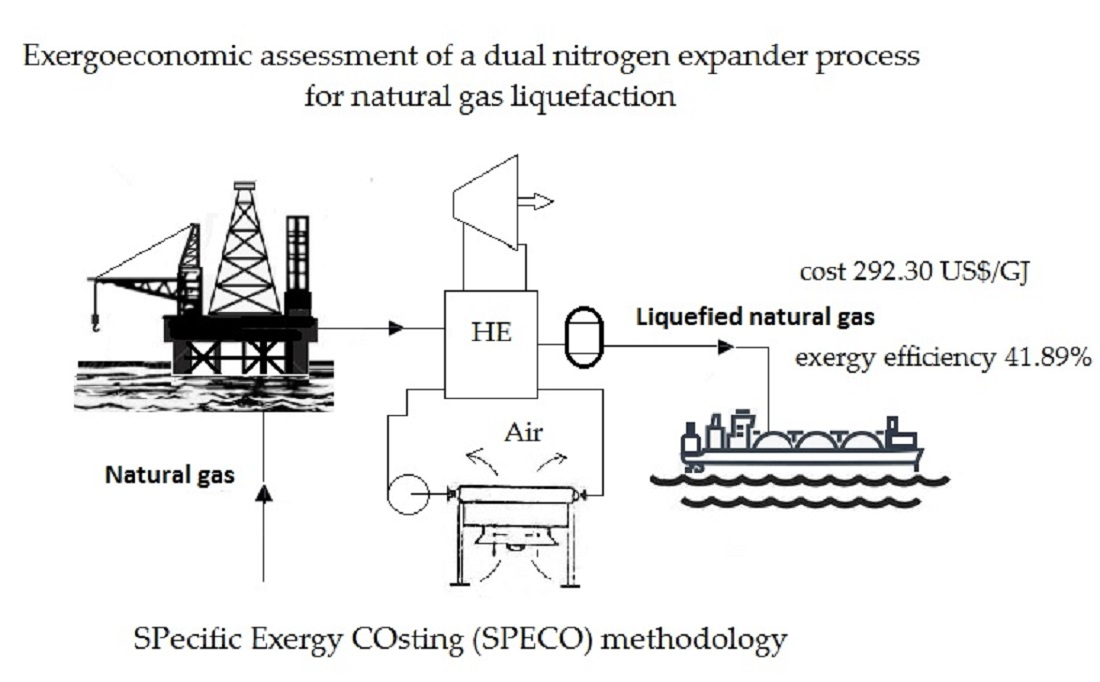
The cryogenic industry has been experiencing continuous progress in recent years, primarily due to the global development of oil and gas activities. Natural gas liquefaction is a cryogenic process, with the refrigeration system being crucial to the overall process. The objective of the study presented herein is to carry out an exergoeconomic assessment for a dual nitrogen expander process used to liquefy natural gas, employing the SPecific Exergy COsting (SPECO) methodology. The air coolers and throttling valve are dissipative components, which present fictitious unit cost rates that are reallocated to the final product (Liquefied Natural Gas). The liquefaction process has an exergy efficiency of 41.89%, and the specific cost of liquefied natural gas is 292.30 US$/GJ. It was verified that this cost increased along with electricity. The highest exergy destruction rates were obtained for Expander 1 and Air cooler 2. The highest average cost per exergy unit of fuel was obtained for the vertical separator, followed by Air coolers 1 and 2. An assessment of the exergoeconomic factor indicated that both expanders could benefit from a decrease in exergy destruction, improving the exergoeconomic performance of the overall system. Regarding the relative cost difference, all compressors presented high values and can be enhanced with low efforts.

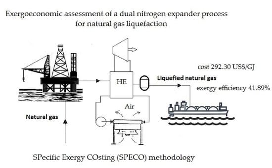
1. Introduction

Energy transition refers to significant structural changes in how energy is used; throughout history, these changes have been driven by the availability of different fuels (and the associated demands). Recognizing that the widespread, indiscriminate use of fossil fuels is the major contributor to climate change, collective global efforts must focus on changing how energy is utilized [1].

The energy transition process has deaccelerated due to the crisis associated with the COVID-19 pandemic, but there is still pressure to shift energy systems away from carbon-intensive hydrocarbons towards low-carbon sources. The strategies to mitigate ever-increasing carbon emissions include incorporating renewable resources, combined energy production schemes, and improving the energy efficiency of current fossil fuel processes through economic and ecological strategies.

The demand for natural gas is expected to grow by 1.6% per year, reaching 25% of the global energy demand in 2030 [2]. Enhancements in the ecological performance of natural gas activities have been the focus of several studies, and Cavalcanti et al. [3] listed some studies that focused on Life Cycle Assessments and ecological performance. One of the issues associated with natural gas is the geographical mismatch between reservoirs and consumer centers, which has led to an increase in global natural gas trade [4] and highlights the need for its transportation.

There are two leading options for the transportation of natural gas: gaseous or liquefied natural gas (LNG). In the latter, natural gas is condensed by cooling it under −162 °C (reducing its volume by a factor of 600) [2]. The liquefaction process of natural gas is energy-intensive, with margins for improvement. As mentioned by Khan et al. [5], the efficient design and operation of LNG facilities is particularly rewarding due to its energy- and cost-intensive nature.

There are three types of LNG technologies: cascade, mixed refrigerant, and expander-based. The differences are complexity-related: cascade employs three separate cycles, mixed refrigerant uses a single cycle, and the expander-based technology utilizes a single cycle with pure refrigerant for [6]. A detailed description of these processes is presented by Lim et al. [7]. Expander-based technologies can employ nitrogen or methane, and its phase remains unchanged, yielding a low-complexity configuration with less equipment. However, expander-based technologies require higher specific power [5].

The nitrogen expansion procedure is adequate for small-scale LNG plants because of its simplicity, quick startup, and straightforward maintenance [8]. As the liquefaction and refrigeration stages are responsible for 42% of the total costs of an LNG system [9], research efforts have been focusing on identifying performance improvement opportunities for LNG processes. For these small-scale LNG production plants, the nitrogen expansion liquefaction process is a good solution and has been widely adopted. More specifically, the compact LNG (cLNG) process uses pure nitrogen and operates at two pressure levels to increase thermodynamic efficiency, employing self-cooling and turboexpanders [7,10].

There have been some studies focused on the improvement of cLNG technologies, however, as mentioned by [3], thermodynamic and environmental assessments are not sufficient on their own and can be complemented by exergy assessments. Regarding more recent studies, Moein et al. [11] used a genetic algorithm to minimize the energy consumption of a nitrogen double turbo-expander cycle. When methane concentration was 26 ± 1 mol percent, the energy consumption was minimum and 8% lower than the reference case (pure nitrogen). Qyyum et al. [12] proposes an innovative two-phase expander LNG process that uses ethane and nitrogen, and develops energy, exergy, and economic assessments. The results indicated 47.83% energy savings with 55.25% less exergy destruction, and 24.12% less total costs than the reference nitrogen single expander process. Qyyum et al. [13] proposed a propane-nitrogen two-phase expander cycle to liquefy natural gas, and carried out optimization with particle swarm algorithm along with exergy analysis. Significant decreases in the specific compression power can be achieved by reducing the temperature gradient in the main LNG liquefier, with energy savings of 46.4% when compared to the conventional single expander LNG process. Palizdar et al. [14] simulated a mini-scale nitrogen dual expander natural gas liquefaction process, and carried out optimization regarding the minimization of specific energy consumption and total exergy destruction. The results demonstrated that the consideration of exergy within optimization yielded better results, with 7.1% less energy consumption, 9.5% less exergy destruction, and exergy efficiency 4.4% higher. Jin et al. [15] discussed a liquefaction process that used propane-free mixed refrigerant and nitrogen expander cycles, with an increase of 27.15% in liquefaction efficiency and an increase of 14.92% in exergy efficiency, in comparison with the baseline. In exergoeconomic assessments, the relative cost difference is a parameter that identifies the potential of improvement of each component. Higher values of relative cost difference indicate that less effort is required for optimization of the system. The values in scientific literature vary between 1 and 1000%: In [16], values ranged from 6% to 367%; in [17] values varied between 14% and 620%; and in [18], values ranged from 34 to 147%.

Although there are some examples of exergoeconomic assessments of LNG technologies, such as [16] (natural gas liquefaction and nitrogen removal) and [19] (mixed fluid cascade), there is scarce scientific literature on exergoeconomic studies on nitrogen expander processes, for which Palizdar et al. [20] applied conventional and advanced exergoeconomic and identified high exergy destruction costs for expanders and heat exchangers. This technology, along with single mixed-refrigerant, dominate the small-scale plant capacity range (50,000 to 500,000 gallons per day) of LNG [21].

This is the first study to apply the SPecific Exergy COsting (SPECO) exergoeconomic method to a dual nitrogen expander process. Recognizing that LNG production is a cryogenic process and that the refrigeration system is the most critical section, the objective of this study is to carry out a thermodynamic assessment, with detailed explanations and correction of data found in existing scientific literature, followed by an exergoeconomic assessment based on the SPECO method.

The major contribution of the study presented herein is the development of an exergoeconomic model for the liquefaction of natural gas and a detailed, step-by-step application of the SPECO approach to cryogenic heat exchangers and dissipative components. A scientifically sound methodology to calculate the cost of air coolers is presented, to overcome the issues associated with the overvaluation of component costs. Establishing the cost of natural gas liquefaction is crucial to the selection of the best transportation from offshore platforms to shore, which can encompass pipelines or tanker ships.

2. Materials and Methods

Natural gas is a mixture of hydrocarbon gases; it is mainly composed of methane, with low concentrations of ethane, propane, butane, pentane, and other gases such as nitrogen and carbon dioxide [22]. The liquefaction process is helpful in transporting natural gases due to the reduction of its specific volume when transformed into liquid [23].

The process principle is expanding a stream from high pressure to a cryogenic temperature at low pressure. This initial condition is above the critical pressure and below the critical temperature. The pressure reduction liquefies the fluid, as the final temperature is lower than the saturated temperature corresponding to the final pressure.

Table 1. Critical point and saturated temperature of some hydrocarbons.

Gas	T Crit [°C] *	P Crit [bar] *	T Sat at 2.53 bar [°C] *	Molar Percentage [%] **	Mass Percentage [%]
Methane CH4	−82.59	45.99	−149.10	92.94	87.35
Ethane C2H6	32.18	48.72	−69.73	3.00	5.29
Propane C3H8	96.68	42.47	−19.05	0.48	1.24
Iso-butane C4H10	134.70	36.40	14.29	0.06	0.20
n-butane C4H10	152.00	37.96	26.21	0.08	0.27
Nitrogen N2	−147.00	33.98	−187.10	3.44	5.65

* [22]; ** [20].

shows the composition of some hydrocarbons, the critical points, and the saturation temperature at 2.53 bar. Composition on a mass basis was calculated by the authors, based on the molar composition [20]. The remaining properties were obtained from the databases within EES [24].

Nitrogen has the lowest critical and condensation temperatures, which is why it is used in gas turbines for power production purposes. The final temperature of liquid natural gas should be below the saturation temperature of methane, −149.1 °C for 2.53 bar. The quality of natural gas can vary, depending on the location and process employed. The natural gas originating from platforms presents a high content of nitrogen, which is the case of this study. The composition of purified natural gas, ready for combustion, presents a much lower nitrogen content, such as 1.28% in volume base or 2.03% at mass base [25].

2.1. Liquefaction Process

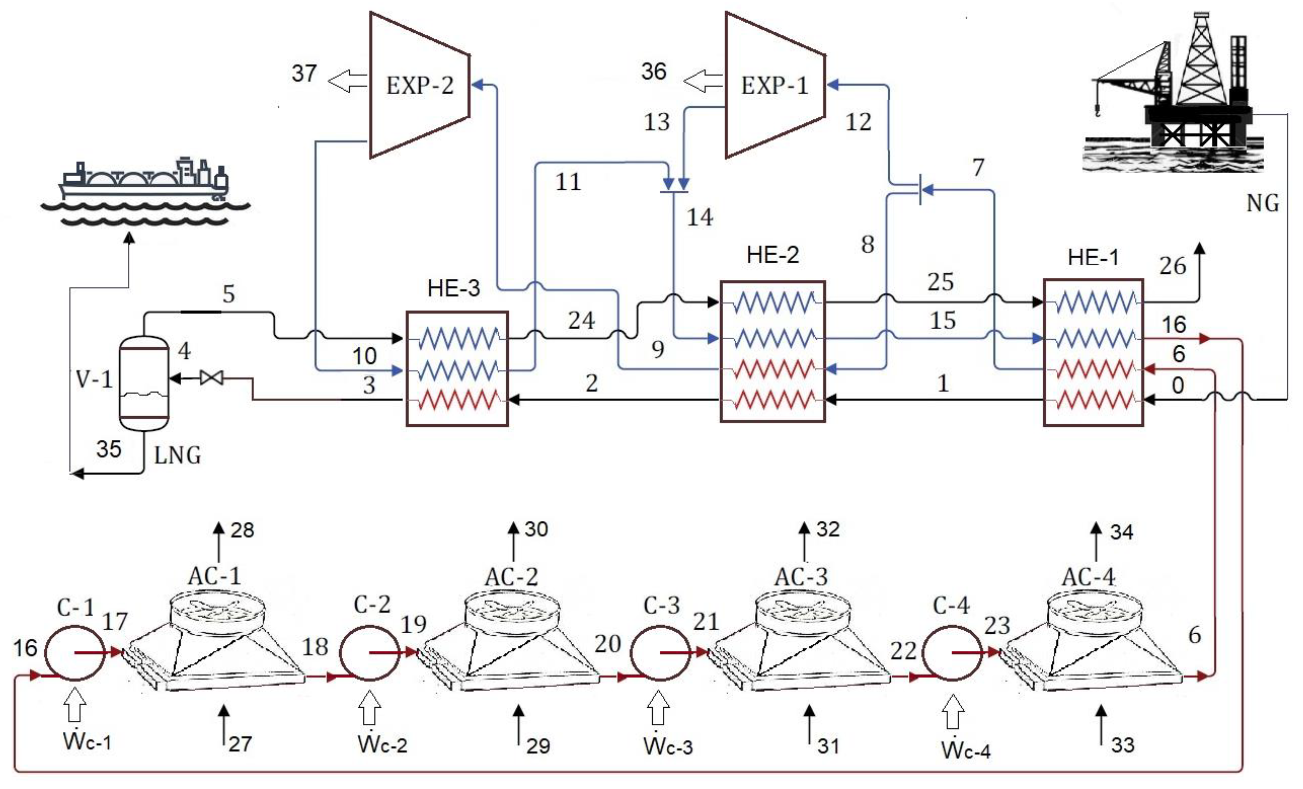
Nitrogen expander processes for natural gas liquefaction are frequently employed in offshore platforms due to their simplicity and safety [23]. The expanders supply part of the power required by the nitrogen compressors. A scheme of the process is shown in Figure 1.

The pressurized natural gas (above critical pressure) at point 0 enters the heat exchangers 1, 2, and 3 and is cooled from 35 °C to −143 °C. The throttling valve reduces the pressure from 58.50 bar to 2.53 bar, liquefying the mixture of natural gas except for nitrogen, which remains gaseous. The lowest temperature of natural gas occurs after the throttling valve, before phase separation. The liquid natural gas exits the vertical separator at point 35, and the gaseous nitrogen flows to three heat exchangers until its disposal into the environment. A secondary system (with compressors, air coolers, and expanders) is used to produce power and refrigerate the liquid natural gas in the heat exchangers. The secondary system uses nitrogen as a working fluid. At the expander outlet, the refrigerant is cool. The refrigerant from the secondary system (at low pressure) and the nitrogen from the vertical separator are heated while passing through the heat exchangers. In these heat exchangers, the natural gas is cooled until its liquefaction. The refrigerant of the secondary system exits HE-1 at point 16 and undergoes a four-stage compression with intercoolers.

The pairs of compressor/air coolers alternate from compressor C-1 at 5.95 bar until the compressor C-4, with the air cooler AC-4 in the end, achieving 40 bar. The refrigerant of the secondary system returns to HE-1 at point 6 and is cooled before entering both expanders. The refrigerant of the secondary system is separated in two flows, one entering expander 1 and the remainder into expander 2. The two expanders produce a share of the power consumed in the compressors. Part of the refrigerant from the secondary system, which exits expander 2, is heated in the heat exchanger (HE-3) before joining the first flow that exits expander 1. The combined mixture of secondary system refrigerant flows into heat exchangers 2 and 3, and the process is restarted. The heat exchangers are the multi-stream type used in cryogenic processes.

For the thermodynamic model, the following assumptions were employed:

• Steady-state;
• Compression and expansion processes were adiabatic;
• Isenthalpic expansions occurred in expansion devices;
• Effects of kinetic and potential energy were not considered.

2.2. Exergy Analysis

An exergy analysis identifies the source and magnitude of losses or exergy destruction, providing relevant information on the quality of energy and process efficiency [26]. The specific exergy can encompass chemical and physical components. Physical exergy (ex^Ph) is evaluated based on the dead state as expressed by Equation (1).

ex^Ph = h − h₀ − T₀ (s − s₀)

(1)

where the dead state refers to the environmental conditions, represented by subscript 0; T is temperature (K), s is entropy (kJ/kg·K), and h is enthalpy (kJ/kg).

The natural gas liquefaction process has no chemical reactions, and therefore its chemical exergy is negligible.

The exergy analysis is based on exergy balances, which originate from the first and second laws of thermodynamics. The exergoeconomic method herein employed is the SPecific Exergy COsting (SPECO) [27]. In SPECO, the component should have a thermodynamic product—this means a productive unit must have a purpose (product) and consume any fuel. SPECO was initially proposed in [28] and then systematically presented by Lazzaretto and Tsasaronis [27]. The definitions of fuel and product can include all the exergy components (mechanical, thermal, and chemical). The two fundamental principles are the Fuel (F) and Product (P) principles, which are defined considering the purpose of a component.

According to SPECO [27], the product is defined as equal to the sum of all the exergy values to be considered at the outlet plus all the exergy increases between inlet and outlet that are following the purpose of the component. The fuel is defined as equal to all the exergy values to be considered at the inlet plus all the exergy decreases between inlet and outlet minus all the exergy increases that are not following the component’s purpose.

The exergy balance considers the exergy of the fuel (${\dot{\mathrm{E}}\mathrm{x}}_{\mathrm{F}}$), product (${\dot{\mathrm{E}}\mathrm{x}}_{\mathrm{P}}$), and its destruction (${\dot{\mathrm{E}}\mathrm{x}}_{\mathrm{D}}$), as shown in Equation (2).

$${\dot{\mathrm{E}}\mathrm{x}}_{\mathrm{F}}={\dot{\mathrm{E}}\mathrm{x}}_{\mathrm{P}}+{\dot{\mathrm{E}}\mathrm{x}}_{\mathrm{D}}$$

(2)

The exergy efficiency (ε) is an important parameter, being the ratio between the exergy of products (${\dot{\mathrm{E}}\mathrm{x}}_{\mathrm{P}}$) and fuels (${\dot{\mathrm{E}}\mathrm{x}}_{\mathrm{F}}$), according to Equation (3).

$$\mathsf{\epsilon }=\frac{{\dot{\mathrm{E}}\mathrm{x}}_{\mathrm{P}}}{{\dot{\mathrm{E}}\mathrm{x}}_{\mathrm{F}}}$$

(3)

Each component should have its efficiency and exergy destruction evaluated. The exergy balances are shown in Appendix A.

2.3. Exergoeconomics

The exergoeconomic analysis is used to unravel and understand the cost formation process. The costs are defined by systematically registering exergy and cost additions as well as removals from each material and energy stream. Exergoeconomics was developed by [29] and combines the exergy rate with economics principles. The thermoeconomic balance is expressed by Equation (4).

$${\mathrm{c}}_{\mathrm{P}}·{\dot{\mathrm{E}}\mathrm{x}}_{\mathrm{P}}={\mathrm{c}}_{\mathrm{f}}·{\dot{\mathrm{E}}\mathrm{x}}_{\mathrm{F}}+\dot{{\mathrm{Z}}_{\mathrm{i}}}$$

(4)

${\mathrm{c}}_{\mathrm{P}}$ and ${\mathrm{c}}_{\mathrm{F}}$ are the average costs per exergy unit of product and fuel, respectively, and $\dot{\mathrm{Z}}$ is the capital cost of component i. The latter is converted into the cost rate considering the capital recovery factor (CRF), as shown in Equation (5).

$${\dot{\mathrm{Z}}}_{\mathrm{i}}={\mathrm{Z}}_{\mathrm{i}}·\mathrm{CRF}·\mathsf{\phi }$$

(5)

φ represents the maintenance factor (herein considered as 1.06). CRF is an economic parameter that depends on the interest rate (in) and the estimated equipment lifetime (n_y). The component costs are shown in Appendix B.

According to [25], the CRF can be calculated by Equation (6).

$$\mathrm{CRF}={\left[\frac{{\mathrm{q}}^{\left({\mathrm{n}}_{\mathrm{y}}+{\mathrm{n}}_{\mathrm{cp}}\right)}-1}{\left(\mathrm{q}-1\right)·{\mathrm{q}}^{\left({\mathrm{n}}_{\mathrm{y}}+{\mathrm{n}}_{\mathrm{cp}}\right)}}-\frac{{\mathrm{q}}^{{\mathrm{n}}_{\mathrm{cp}}}-1}{\left(\mathrm{q}-1\right)·{\mathrm{q}}^{{\mathrm{n}}_{\mathrm{cp}}}}\right]}^{-1}·\frac{1}{{\mathrm{n}}_{\mathrm{hour}}}$$

(6)

$$\mathrm{q}=\left(1+\frac{\mathrm{in}}{100}\right)\left(1+\frac{\mathrm{ri}}{100}\right)$$

(7)

n_y is the lifetime of equipment (25), n_cp is the number of years of construction (2), n_hour is the annual operation hours (7446), in is the interest rate [%] taken as 10%, and ri is the rate of inflation [%] considered as 1.5%. Regarding total investment costs, in addition to purchased equipment costs (PEC, capital costs), direct and indirect costs can also apply. Following [29], direct costs include installation costs (50% of PEC), piping costs (30% of PEC), and instrumentation and control costs (20% of PEC). Indirect costs include engineering and supervision costs (50% of PEC), and construction costs (15% of direct costs) [29]. Thus, the total investment cost is the cost of all purchased equipment multiplied by a cost factor of 2.80.

The exergoeconomic factor (f) reveals which piece of equipment should be the focus of improvements, regarding economically feasible investments. f is calculated by Equation (8).

$$\mathrm{f}=\frac{{\dot{\mathrm{Z}}}_{\mathrm{i}}}{{\dot{\mathrm{Z}}}_{\mathrm{i}}+{\mathrm{c}}_{\mathrm{F}}·\left({\dot{\mathrm{E}}\mathrm{x}}_{\mathrm{D}}\right)}$$

(8)

A low value of f indicates that overall cost savings can be achieved by improving the efficiency of the component, which means to decrease its exergy destruction even at the expense of an increase in capital costs.

The relative cost difference for a component k (r_k) is the relative increase in the average cost per exergy unit between fuel and product of component, and evaluated as shown in Equation (9).

$${\mathrm{r}}_{\mathrm{k}}=\left(\frac{{\mathrm{c}}_{\mathrm{P}}-{\mathrm{c}}_{\mathrm{F}}}{{\mathrm{c}}_{\mathrm{F}}}\right)$$

(9)

The exergoeconomic balances are shown in Appendix C.

The cost of natural gas is 1.73 × 10⁻³ US$/kg at point 0, and the electricity cost is 0.017 US$/kWh (4.72 US$/GJ) [20]. The cost of natural gas from a platform is lower than the cost of purified natural gas because it is composed only of exploration and production costs. The cost of ready-to-use natural gas can be as high as 1.74 US$/kg [25], which has additional costs such as transmission, purification, and distribution. More information about the stages of natural gas life cycle can be consulted in [3].

2.4. Heat Exchanger

The concept of fuel and product in heat exchangers that work with temperatures below the dead state has some nuances. This section presents a detailed evaluation of physical exergy. Considering temperature, when a stream is at the dead state temperature, its physical exergy is null. When the stream’s temperature is above or below the dead state temperature, it has positive physical exergy. Depending on the temperature change, the product and fuel exergies can be calculated by subtracting or adding two points or one point.

Physical exergy is affected by pressure. If the pressure is equal to the dead state pressure, its effect is null. If pressure is above or below the dead state pressure, its value is positive or negative, respectively. This usually occurs in absorption cooling systems that employ LiBr solutions. This was discussed in detail by [30].

As the temperature has a more dominant effect on physical exergy, it is employed in the definition of fuel and product exergy. The concept of fuel and product was previously stated by [27]. Additionally, these concepts can be found in [31,32] regarding changes in the temperatures of hot and cool fluids.

Table 2. SPECO method applied to heat exchangers.

Case	Diagram	Exergy and Exergoeconomic Balances		Aux Equations
		Product	Fuel
(a)		${\mathrm{Ex}}_{\mathrm{P}}={ \mathrm{Ex}}_4-{\mathrm{Ex}}_3$ ${\mathrm{C}}_{\mathrm{P}}={\dot{\mathrm{C}}}_4-{\dot{\mathrm{C}}}_3$	${\mathrm{Ex}}_{\mathrm{F}}={ \mathrm{Ex}}_1-{\mathrm{Ex}}_2$ ${\mathrm{C}}_{\mathrm{f}}={\dot{\mathrm{C}}}_1-{\dot{\mathrm{C}}}_2$	F: c1 = c2
(b)		${\mathrm{Ex}}_{\mathrm{P}}={ \mathrm{Ex}}_4$ ${\mathrm{C}}_{\mathrm{P}}={\dot{\mathrm{C}}}_4$	${\mathrm{E}}_{\mathrm{F}}=({\mathrm{Ex}}_1-{\mathrm{Ex}}_2)+{\mathrm{Ex}}_3$ ${\mathrm{C}}_{\mathrm{f}}={\dot{\mathrm{C}}}_1-{\dot{\mathrm{C}}}_2+{\dot{\mathrm{C}}}_3$	F: c1 = c2 Or ${\mathrm{c}}_3=\frac{{\dot{\mathrm{C}}}_1-{\dot{\mathrm{C}}}_2}{({\mathrm{E}}_1-{\mathrm{E}}_2)}$
(c)		${\mathrm{Ex}}_{\mathrm{P}}={ \mathrm{Ex}}_2+{\mathrm{Ex}}_4$ ${\mathrm{C}}_{\mathrm{P}}={\dot{\mathrm{C}}}_2+{\dot{\mathrm{C}}}_4$	${\mathrm{Ex}}_{\mathrm{F}}={ \mathrm{Ex}}_1+{\mathrm{Ex}}_3$ ${\mathrm{C}}_{\mathrm{f}}={\dot{\mathrm{C}}}_1+{\dot{\mathrm{C}}}_3$	P: c2 = c4
(d)		${\mathrm{Ex}}_{\mathrm{P}}={ \mathrm{Ex}}_2$ ${\mathrm{C}}_{\mathrm{P}}={\dot{\mathrm{C}}}_2$	${\mathrm{Ex}}_{\mathrm{F}}={ \mathrm{Ex}}_1+\left({\mathrm{Ex}}_3-{\mathrm{Ex}}_4\right)$ ${\mathrm{C}}_{\mathrm{f}}={\dot{\mathrm{C}}}_1+{\dot{\mathrm{C}}}_3-{\dot{\mathrm{C}}}_4$	F: c3 = c4 Or ${\mathrm{c}}_1=\frac{{\dot{\mathrm{C}}}_3-{\dot{\mathrm{C}}}_4}{({\mathrm{E}}_3-{\mathrm{E}}_4)}$
(e)		${\mathrm{Ex}}_{\mathrm{P}}={ \mathrm{Ex}}_2-{\mathrm{Ex}}_1$ ${\mathrm{C}}_{\mathrm{P}}={\dot{\mathrm{C}}}_2-{\dot{\mathrm{C}}}_1$	${\mathrm{Ex}}_{\mathrm{F}}={ \mathrm{Ex}}_3-{\mathrm{Ex}}_4$ ${\mathrm{C}}_{\mathrm{f}}={\dot{\mathrm{C}}}_3-{\dot{\mathrm{C}}}_4$	F: c3 = c4

shows the definition of fuel and product for the heat exchanger, considering different dead state temperatures. T1 and T3 are the input temperatures of the hot and cool fluid, respectively, and T2 and T4 are the output temperatures of the hot and cool fluid, respectively. The arrow indicates the direction of each fluid, i.e., from T1 to T2 and from T3 to T4. The red line refers to the definition of fuel stream, where the exergy is reduced between the inlet and the outlet. The black line refers to the definition of product stream, where the exergy is increased between inlet and outlet [27]. The dead state temperature (To) is the gray line.

It must be noted that as we move further (above or below) the dead state temperature (To), the specific exergy becomes higher. Temperatures below the dead state temperature (To) have positive specific exergy; any temperature equal to the value of dead state temperature (To) has no exergy.

When defining the fuel and product of a heat exchanger, these are related to the exergy analysis of the component. The objective of a heat exchanger can be to heat or cool a fluid; however, when carrying out an exergy analysis, the product is defined as an increasing exergy rate or output exergy, which can be different from its objective.

Working with pressures above or equal to atmospheric pressure, even below the dead state temperature, yields a positive exergy rate.

The golden rule to solve the set of balance equations is that when there is more than one output stream, the number of auxiliary equations is (n − 1). For all cases presented in Table 2, there are four streams (two inputs, two outputs, and therefore one auxiliary equation is necessary (2 − 1 = 1)).

Case (a): All temperatures are above the dead state temperature. The product and fuel are defined by differences. The specific enthalpy and exergy of point 1 are higher than point 2; therefore, their enthalpy and exergy were reduced between the input and output streams. The fluid 1–2 in red is the fuel, according to the SPECO definition. The heat rate and exergy rates are transferred from the hot fluid to the cool fluid. The hot fluid decreases its exergy rate and the cool fluid increases its exergy rate. The auxiliary equation follows the fuel rule, where the specific costs of fuel fluid of input and output are equal.

Case (b): Temperature T3 is below the dead state temperature. Point 3 has a positive exergy rate. As fluid 3–4 crosses the dead state temperature, the input is the fuel and the output is the product. The product in black is the output stream of cool fluid, for which its specific exergy is associated with temperature (T4). The fuel (red line) is similar to case (a), and defined by the exergy rate differences of hot fluid plus the exergy rate of input stream of cool fluid associated with T3. The definition of fuel as input and product as output is used when the fluid crosses the dead state temperature. The auxiliary equation follows the fuel rule.

Case (c): Both fluids cross the dead state temperature. Temperatures T2 and T3 are below the dead state temperature. The product (black line) is the exergy rate of the output stream of cool fluid (T4) plus the exergy rate of the output stream of hot fluid (T2). The product (black line) is the exergy rate associated with temperature T4 plus the exergy rate associated with temperature T2. The fuels are defined by the exergy rate of input stream of hot fluid (T1) plus the exergy rate of input stream of cool fluid (T3). The fuels (red line) are the exergy rate associated with temperature T1 plus the exergy rate associated with temperature T3. The auxiliary equation follows the product rule, where the specific costs of products are equal.

Case (d): Only temperature T1 is above the dead state temperature. The product (black line) is the exergy rate of the output stream of hot fluid, for which exergy is associated with temperature T2. The fuel (red line) is defined by the exergy rate difference of cool fluid plus the exergy rate of input stream of hot fluid stream (exergy rate T3 minus exergy rate T4 plus exergy rate T1). The exergy rate at point 3 is higher than the exergy rate at point 4; the specific exergy of fluid 3–4 (cool fluid) is reduced and defined as part of fuel. However, fluid 3–4 (cool fluid) has its temperature increased. The auxiliary equation follows the fuel rule.

Case (e): All temperatures are below the dead state temperature. The product and fuel are defined by differences. The fluid 3–4 (cool fluid) behaves similarly to case (d), where it is fuel. The heat rate is transferred from the hot fluid to the cool fluid; however, the exergy rate is transferred from the cool fluid to the hot fluid. The hot fluid (fluid 1–2) increases its exergy rate; however, it reduces its temperature, losing heat rate. The cool fluid (fluid 3–4) decreases its exergy rate but it increases its temperature by receiving heat rate. The auxiliary equation follows the fuel rule. This opposite effect occurs at lower temperatures, such as cryogenic processes or ice production.

The SPECO approach addresses dissipative components [27] by referring to the destruction of exergy within a component without gaining something thermodynamically useful, i.e., without any product. Examples: gas cleaning units, throttling valves, and coolers operating at temperatures above the ambient temperature. The operation of dissipative components is only meaningful when considered in the context of the overall thermal system [27]. A cooler located immediately before a compressor helps reduce the power consumed for its operation. All costs associated with owning and operating this cooler (dissipative component) are then directly allocated to the compressor (the component served by the cooler).

An air cooler is a dissipative component with inlet and outlet streams associated with the primary working fluid and with an auxiliary working fluid (environment air). The exergy of the primary working fluid at the outlet is lower than at the inlet, due to exergy destruction within the dissipative component and exergy transfer through the auxiliary working fluid. The F principle states that the cost per exergy unit of the main working fluid remains constant between the inlet and outlet. The cost rate associated with the auxiliary working fluid, called fictitious unit for distributing the cost rate (${\dot{C}}_{dif,dc}$), is the output of air flow and should be allocated to the compressor. There are three possibilities of cost rate allocation in a fictitious unit [27]:

(a)

to the component(s) served by the dissipative component,

(b)

to the productive component(s) responsible for the use of the dissipative component, or

(c)

to the final product(s) of the overall system.

The other dissipative component is the throttling valve, which has its fictitious unit cost rate reallocated to the final product (LNG).

2.5. Air Cooler Design

Air coolers should present low air velocity across the bundles to hold pressure losses and power at the fan. Higher air velocity increases pressure losses and the power consumed. However, lower air velocity also increases the required area and capital costs. The heat transfer (Q) of air coolers, in kW, is evaluated by Equation (10).

$$\mathrm{Q}=\mathrm{U}·\mathrm{A}·\mathrm{f}·\mathrm{LMTD}$$

(10)

The overall heat transfer coefficient (U) is 0.2 [kW/m²·K] according to [33,34]; A is the area, and f is the correction factor of the configuration, taken as 0.95 for two rows of tubes and single pass. LMTD is the log-mean temperature difference for counter-current flow [°C]. The output air temperature should not be higher than 50 °C to prevent damage to the operator, such as burns.

The power consumed ($\dot{\mathrm{W}}, \mathrm{in} \mathrm{kW}$) is estimated by the volumetric flow rate of air ($\dot{\mathrm{V}}$) as shown by Equation (11).

$$\dot{\mathrm{W}}=\frac{\mathsf{\gamma }·\dot{\mathrm{V}}·\mathrm{H}}{\mathsf{\eta }}=\frac{\dot{\mathrm{V}}·\Delta \mathrm{P}}{\mathsf{\eta }}$$

(11)

$\dot{\mathrm{V}}$ is the air flow rate [m³/s], ΔP is the pressure loss, and η is the efficiency as 75%. The volumetric flow rate of air is used to determine the heat transfer (expressed in kW) as given by Equation (12).

$$\mathrm{Q}=\mathsf{\rho }·\dot{\mathrm{V}}·\left({\mathrm{h}}_{\mathrm{air},\mathrm{out}}-{\mathrm{h}}_{\mathrm{air},\mathrm{in}}\right)$$

(12)

ρ is the specific mass of environmental air [kg/m³].

Pressure loss is a relevant parameter when designing air coolers, as it defines the power consumed. The fan should deliver the required amount of air at specific operation conditions and avoid excessive noise. According to [35], the optimized design can be obtained, when the heat duty is met, such that limits imposed on the maximum allowable pressure drop as 0.250 kPa (1.0 in water column) and/or flow velocity are respected. This threshold value limits the required power, but increases operation costs associated with electricity demand. However, a rational evaluation of the heat transfer area keeps the investment costs within acceptable values. The total cost, composed of operation and investment costs, should be (ideally) minimum.

3. Results and Discussions

Model validation was carried out considering the specific exergy at each point and the differences were evaluated as shown in

Table 3. Model validation.

Point	e [20] [kJ/kg]	e This Work [kJ/kg]	Δe [%]	Point	e [20] [kJ/kg]	e This Work [kJ/kg]	Δe [%]
0	574.6	575.5	0.16	14	205.3	207.0	0.84
1	573.8	578.7	0.85	15	167.8	169.1	0.75
2	733.1	732.7	−0.05	16	156.7	158.0	0.84
3	942.5	941.7	−0.09	17	183.3	184.7	0.75
4	910.4	941.4	3.29	18	174.9	176.2	0.75
5	283.2	179.6	−57.71	19	242.4	243.7	0.55
6	324.4	326.4	0.61	20	227.0	228.5	0.64
7	324.9	326.8	0.59	21	291.3	292.9	0.55
8	324.9	326.8	0.59	22	278.1	279.8	0.61
9	353.0	354.9	0.53	23	335.1	337.0	0.55
10	276.4	279.9	1.25	24	223.4	141.9	−57.44
11	204.1	205.7	0.76	25	75.0	49.5	−51.64
12	324.9	326.8	0.59	26	2.4	2.6	8.47
13	208.9	210.7	0.85	35	973.2	1013.0	3.93

. Because additional points were considered herein compared to [20], numeration was adjusted, and some points have no value.

The difference of specific exergy changes from −0.09 to 1.25 %. However, at point 4, the difference increases to 3.29%. At this point, the mixture of natural gas is liquid, except for nitrogen, which is gaseous. Points 5, 24, 25, and 26 refer to gaseous pure nitrogen and the differences are highest, changing from 8.47 to −57.71%. The evaluation of specific exergy of pure nitrogen could have had issues, or there are other components at these points, which are not explained by [20]. The LNG at point 35 has a slight difference of 3.93%. Despite the higher differences obtained for pure nitrogen, the specific exergy evaluation of the model presented good accuracy.

The initial conditions of mass flow, pressure, and temperature follow [20].

Table 4. Thermodynamic, exergy, and exergoeconomic performance data.

Point	T [°C]	P [bar]	$\dot{\mathbf{m}}$ [kg/h]	$\dot{\mathbf{E}}$ [kW]	c [US$/GJ]	$\dot{\mathbf{C}}$ [US$/h]
0	35.00	60.00	461.8	73.82	3.01	0.80
1	−8.15	59.50	461.8	74.31	235.70	62.98
2	−87.14	59.00	461.8	91.58	277.80	93.98
3	−155.00	58.50	461.8	128.00	281.00	129.50
4	−157.40	2.53	461.8	124.00	281.00	125.40
5	−157.40	2.53	26.1	1.36	281.00	1.38
6	40.00	40.02	4457.0	388.60	263.70	383.60
7	−8.15	39.52	4457.0	389.40	235.70	343.30
8	−8.15	39.52	1824.0	157.40	235.70	140.50
9	−87.14	39.02	1824.0	172.20	251.60	162.90
10	−156.50	7.55	1824.0	138.70	251.60	128.50
11	−86.44	7.30	1824.0	98.97	251.60	94.42
12	−8.15	39.52	2633.0	232.00	235.70	202.80
13	−100.60	6.95	2633.0	150.00	235.70	130.70
14	−94.99	6.95	4457.0	246.70	244.00	225.20
15	−21.68	6.45	4457.0	201.40	244.00	184.00
16	40.46	5.95	4457.0	188.30	235.70	166.00
17	67.96	7.80	4457.0	219.80	272.60	224.40
18	40.00	7.30	4457.0	209.80	272.60	214.10
19	116.30	13.69	4457.0	290.20	266.60	289.60
20	40.00	13.19	4457.0	272.00	266.60	271.50
21	112.90	24.09	4457.0	348.70	263.20	343.60
22	40.00	23.59	4457.0	333.10	263.20	328.20
23	105.00	40.52	4457.0	401.20	263.70	396.10
24	−140.00	2.03	26.1	1.03	281.00	1.04
25	−50.00	1.53	26.1	0.36	281.00	0.36
26	25.00	1.03	26.1	0.02	0.00	0.00
27	25.00	1.01	8503.0	0.00	0.00	0.00
28	40.00	1.01	8503.0	0.85	0.00	0.00
29	25.00	1.01	14033.0	0.00	0.00	0.00
30	50.00	1.01	14033.0	3.81	0.00	0.00
31	25.00	1.01	13548.0	0.00	0.00	0.00
32	50.00	1.01	13548.0	3.68	0.00	0.00
33	25.00	1.01	12300.0	0.00	0.00	0.00
34	50.00	1.01	12300.0	3.34	0.00	0.00
35	−157.40	2.53	435.7	122.60	283.00	124.90
36				63.57	305.20	72.95
37				28.65	334.10	34.91
38				92.22	314.00	107.90
39					292.30

lists the temperature, pressure, mass flow rate, exergy rate, specific cost, and cost rates.

The throttling valve (between points 3 and 4) reduces pressure from 58.50 bar to 2.53 bar. In [20], the temperature was decreased from −143.0 °C to −152.34 °C with a temperature difference of −9.34 °C. The temperature −152.34 °C was not achieved in the energy balance carried out herein. In scientific literature, natural gas liquefaction processes use input temperatures around −160 °C and reduce the valve temperature of 0.5 to 3 °C [36,37]. Herein, the input and output temperatures of natural gas in the throttling valve are −155 °C and −157.35 °C, respectively.

The mass flow rate of stream at point 5 should be gaseous nitrogen. The mass composition of nitrogen within natural gas is 5.65%, which corresponds to 26.09 kg/h out of 461.78 kg/h. Therefore, the mass flow rate considered herein is 26.09 kg/h (instead of 45.12 kg/h considered by [20]).

The correction of the mass flow rate of nitrogen at point 5 will change the mass flow rate of liquefied natural gas at point 35 and the mass flow rate of the system with refrigerant at points 5, 10, and 14. Some temperatures were recalculated considering the heat exchangers as adiabatic, such as T11, T14, and T16. The minimum pinch point temperatures at the heat exchangers were 0.5, 7.9, and 0.7°C for HE-1, HE-2, and HE-3, respectively. The advantage of exergy analysis is that when there are issues with the heat exchanger pinch point, the value of exergy destruction generated is negative, which is inconsistent. This behavior was reported by [30].

The exergy rates were calculated considering physical exergy, as there is no chemical reaction involved. The power produced in expanders 1 and 2 is 66.39 kW and 29.03 kW at points 36 and 37, respectively. The global power produced in the expanders is 95.42 kW at point 38. The power consumed in refrigerant compressors 1, 2, 3, and 4 is 38.39 kW, 98.37 kW, 93.87 kW, and 83.70 kW, respectively. The total power consumed is 314.3 kW, as the two expanders produce power, and the net power consumed is 218.9 kW. The ratio of power consumed is 69.64%. The heat rates of air coolers 1, 2, 3, and 4 are 36.28 kW, 99.81 kW, 96.35 kW, and 87.48 kW, respectively. These results are similar to [20].

The cost of air coolers is calculated based on their area and evaluated by their performances, i.e., heat rate, Log Mean Temperature Difference (LMTD), and air volumetric flow rate.

Table 5. Performance data and cost of air coolers.

Air Cooler	Q [kW]	LMTD [°C]	$\dot{\mathbf{V}}$ [m3/s]	A [m2]	W [kW]	Z [US$]
1	36.28	20.81	2.036	9.176	0.6788	11,884
2	99.81	34.52	3.360	15.220	1.1200	14,550
3	96.35	33.40	3.244	15.180	1.0810	14,537
4	87.48	30.78	2.946	14.960	0.9818	14,450

shows the heat rate, LMTD, air volumetric flow rate, area, power consumed, and cost of all air coolers.

The input air temperature at the air cooler is 25 °C. The input refrigerant temperatures are 67.96 °C, 116.3 °C, 112.85°C, and 104.99 °C for AC1, 2, 3, and 4, respectively. All output refrigerant temperatures are 40 °C.

In the present work, the output air temperature was assumed as 40 °C for AC1 and 50 °C for AC2, 3, and 4, due to the lower input refrigerant temperature of AC1. These temperatures are used for the evaluation of LMTD. The LMTD values of [20] are 26.47 °C, 42 °C, 40.98 °C, and 38.61°C for AC1, 2, 3, and 4, respectively, and correspond to the output air temperature of 24.32 °C, 25.83 °C, 25.78 °C, and 25.7 °C. As the air flow should be heated in the air cooler, the value of 24.32 °C is not consistent, as it should be higher than 25 °C. The increase in air temperature is very small, around 0.7 to 0.83 °C in [20]. Therefore, the volumetric flow of air and power consumed is high.

The cost of air coolers is area-dependent. The values of air volumetric flow rate and area of [20] were not explicit. In the present work, the power consumed and costs of air coolers (Table 4) are 0.679 kW, 1.120 kW, 1.081 kW, and 0.982 kW, and 11,884 US$; 14,550 US$; 14,537 US$; and 14,450 US$, for AC 1, 2, 3, and 4, respectively. The values of [20] for power are 7.64 kW, 7.63 kW, 8.05 kW, and 7.64 kW, and costs are 137,320 US$; 137,320 US$; 135,823; and 137,261 US$ for AC-1, 2, 3 and 4, respectively. The power consumed and costs of air coolers used herein are not similar to [20], due to the different output air temperatures. Our lower air volumetric flow reduces the power of the fan. The cost of air coolers is based on area, and according to [38], in 2002 the cost of an air cooler with an area of 9.18–15.22 m² (98–164 ft²) was between 20,000 and 25,000 US$. According to [29], the cost restatements of equipment (cost index) should be used with caution when considering periods over 10 years and should not be applied to equipment. Technology improvement and competition significantly affect the price. Inflation increases price while technological advances reduce the price. Hence, an air cooler cost between 11,880 and 14,550 US$ is more reasonable. The value used by [20] (137,000 US$) would correspond to an immense area of 44.83 kft² (4164 m²). AC1 and 2 have different loads, however, they have the same power and cost.

The specific costs of power from expander 1 and 2 are 305.20 US$/GJ and 334.10 US$/GJ, respectively. The average specific cost of power is 314.00 US$/GJ. It is important to note that the cost of the electricity supplied by the electric grid is 4.72 US$/GJ, which is lower than the cost of power produced. This occurs because the purpose of the system is to liquefy natural gas and not to produce electricity. It is a sub-product that reduces the cost of the liquefaction process.

The product of the system is a liquefied natural gas at point 35. Its specific cost is 283.00 US$/GJ. Point 39 is composed of the LNG cost rate of point 35 plus the reallocated fictitious cost rate of the valve plus the cost rate of released nitrogen in the atmosphere at point 26, which yields a specific cost of 292.30 US$/GJ at point 35. The cost rate of air coolers is null for the input and output of environment air (air input at zero cost). However, the output of air should have a cost rate, which is charged to the compressors (the cost rate of air cooler output, which is a dissipative component, was reallocated to the compressors).

Table 6. Exergy and exergoeconomic parameters.

Component	$\dot{E}{\mathbf{x}}_D$ $\left[\mathrm{kW}\right]$	ε [%]	cf [US$/MJ]	cp [US$/MJ]	Z [US$]	$\dot{\mathbf{Z}}$ [US$/h]	f [%]	r [%]
C-1	5.43	85.86	3.29	491.90	758,477	46.89	99.86	14,857.0
C-2	14.77	84.99	3.29	250.80	893,868	55.26	99.68	7525.0
C-3	14.12	84.95	3.29	251.20	885,171	54.72	99.70	7539.0
C-4	12.81	84.70	3.29	266.00	864,888	53.47	99.72	7989.0
Exp-1	18.54	78.17	235.70	305.20	14,342	0.89	5.34	29.5
Exp-2	9.02	76.30	251.60	334.10	7338	0.45	5.26	32.8
HE-1	13.16	98.09	229.70	235.70	58,693	3.63	25.00	2.6
HE-2	13.51	71.59	244.60	435.80	186,703	11.54	49.25	78.2
HE-3	3.89	89.73	251.80	289.90	18,318	1.13	24.29	15.1
AC-1	10.27	7.92	256.30	0.00	11,884	0.73	7.19	-
AC-2	16.05	19.80	251.90	0.00	14,550	0.90	5.82	-
AC-3	13.47	22.12	247.00	0.00	14,537	0.90	6.98	-
AC-4	10.70	24.51	245.70	0.00	14,450	0.89	8.62	-
V-separ	0.01	99.80	281.00	324.70	14,465	0.89	100.00	15.5

shows the exergy destruction rate, exergy efficiency, average cost per exergy unit of fuel and product, cost rate of component, exergoeconomic factor, and cost relative difference.

Expander 1 has the highest exergy destruction rate, followed by air cooler 2. These values are slightly lower than [20], except for the air coolers, which present high differences in the values obtained. All air coolers have the lowest exergy efficiencies, changing from 7.92 to 24.51%. This is due to the low increases in air temperature. These efficiencies are very different from [20], who presented (inconsistent) values from 91.29 to 94.99%.

The average cost per exergy unit of fuel for all compressors is the electricity cost multiplied by the ratio of power consumed (4.72 US$/GJ × 69.64%), 3.29 US$/GJ. The powers produced in the two expanders were distributed to all compressors.

The vertical separator has the highest average cost per exergy unit of fuel, followed by air coolers 1 and 2. The vertical separator only separates the liquefied natural gas from mixture at point 4. As it separates all liquid, there are no margins for improvement. Its fuel is the mass flow of point 5, which has its stream reduced from point 4 to 5. Air coolers 1 and 2 operate in the secondary system and increase the cost rate due to the exergy destruction embedded.

Compressor 1 has the highest average cost per exergy unit of product. Compressor 1 has a low-pressure ratio (P17/P16 = 1.3) in relation to the other compressor, which changes from 1.7 to 1.8. The compressors’ products are the variation of exergy between the output and input. These variations are low and include the reallocated cost rate from the air coolers. Therefore, the average cost per exergy unit of product is higher in relation to the average cost per exergy unit of fuel. The compressors have the highest PEC and cost rates. The value of PEC used herein is similar to [20], except for the four air coolers. The air cost PEC of [20] is much higher than the value employed herein. There are inconsistencies in the output air temperature, power, and pressure, which increased the cost of all air coolers.

The values of average cost per exergy unit of fuel at compressors are similar to [20]; however, all other values and the average cost per exergy unit of product are different. This is due to the considerable cost of PEC. The cost rate of this work is half of the value used by [20]. Other direct and indirect costs could be included in the total cost investment; however, this was not explicit. He and Ju [37] used a cost factor of 6.32, which yielded cost rate values similar to [20] when employed herein. The cost factor used in this work, which considered direct and indirect cost, is 2.80. The cost rate of air coolers is not similar, due to the same reason discussed before.

The exergoeconomic factor indicates that both expanders should receive investments to reduce exergy destruction and improve the exergoeconomic performance of the system. This result is similar to [20]. However, all air coolers have low exergoeconomic factor values. Although air coolers present these low values, they are dissipative components and should not be changed because their function is to destroy exergy by releasing heat. The relative cost difference values are high for all compressors due to the reallocation of the cost rate of air coolers. It means that the compressors can be improved with low effort. The reduction of the relative cost difference is useful for optimization purposes. The values of the relative cost difference (14,857%) are higher than scientific literature data, by 1000%. However, this high value is caused by reallocation. The relative cost difference of [20] reached an extremely high value, 524,603% at the expander, which does not seem consistent.

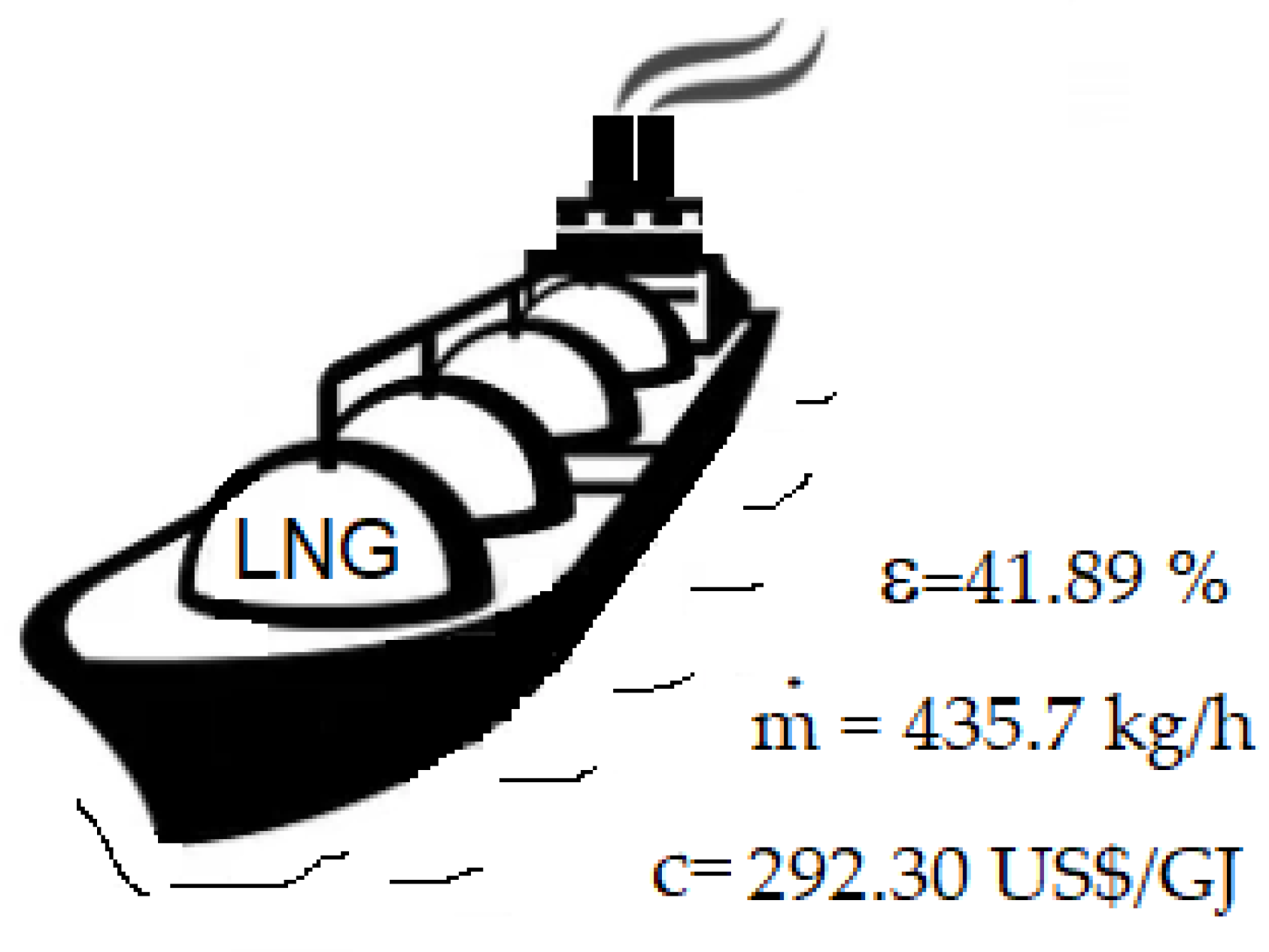
Figure 2 summarizes the results of exergy efficiency, produced mass flow rate, and specific cost of liquid natural gas per exergy unit.

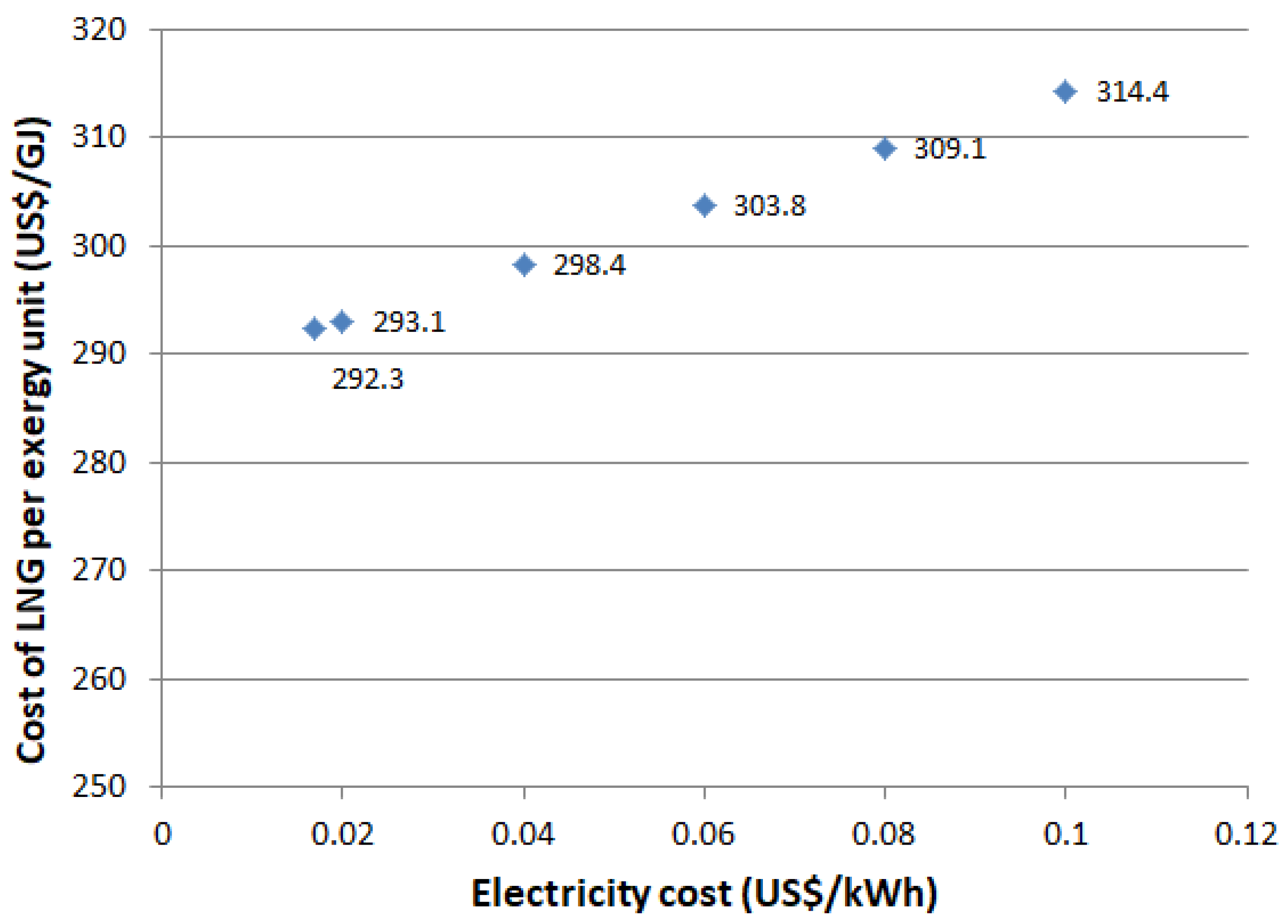
The effect of electricity cost on the specific cost of liquefied natural gas is shown in Figure 3.

The electricity cost changed from 0.017 US$/kWh to 0.10 US$/kWh, leading to an LNG specific cost increase from 292.3 US$/GJ to 314.4 US$/GJ. As the electricity cost increases, the specific cost of LNG also increases. Because electricity is a fuel of the system, it directly affects the specific cost of product (LNG).

Recognizing the importance of natural gas, especially in the aftermath of the COVID-19-related crisis, its exploitation has been in the spotlight when considering cleaner energy targets (i.e., higher carbon intensities associated with oil and coal) [9]. Energy security and exploration of new natural gas reserves have also been relevant since the early 2000s [39]. This highlights the importance of carrying out studies to establish crucial pathways for evaluating activities and processes related to natural gas.

Although mixed-refrigerant cycles dominate at world-class and medium-scale LNG plants, nitrogen expansion cycles started to resurge at small-scale LNG plants [40] and be very utilized in floating LNG production [41]. When comparing single mixed-refrigerant and nitrogen expander cycles, it was observed that there were only minor capital cost differences between the technologies, concluding that a decision is best based on operation costs and operability issues [21] such as the detailed analysis presented herein. The present study determined the most energy-intensive and inefficient components and identified components with the highest cost of exergy destruction.

Finally, the cryogenic industry has continuously progressed in recent years, primarily due to global development and LNG activities. LNG is an economically viable way to transport natural gas over long distances and is responsible for approximately 30% of the international trade [42]. In recent years, the necessity of developing specific studies focused on the oil and gas industry has emerged to deepen knowledge on these energy systems and promote logical operation and better performance. Although there have been studies carried out on the subject, there is a lack of primary data. This study, which should be considered, analyzed, and employed by oil and gas industries, contributes to increase the efficiency of production and identify losses.

4. Conclusions

This is the first study to apply the SPECO exergoeconomic methodology to a dual nitrogen expander process. Detailed explanations are presented herein, along with the correction of thermodynamic parameters found in existing scientific literature.

The exergy analysis results indicate an overall exergy efficiency of 41.89%, and the total exergy destruction rate is 170.1 kW. The essential elements regarding exergy destruction are Expander 1, followed by air cooler 2. Regarding the average cost per exergy unit of fuel, the highest values are associated with the vertical separator and air coolers 1 and 2. Because the vertical separator only separates LNG, there is no potential for improvement. Air coolers 1 and 2 increase the cost rate due to the exergy destruction embedded.

Analysis of the exergoeconomic factor indicates that both expanders should receive investments to reduce exergy destruction and improve the exergoeconomic performance of the system. Although air coolers also present low fk values, they are dissipative components, and it is not cost-effective to focus efforts on improving these (their function is to destroy exergy).

Regarding the relative cost difference, high values were obtained for all compressors, because of the allocation of the cost rates of air coolers. There is potential for improvement, with low efforts, for the compressors. Decreasing the relative cost difference is useful for optimization purposes. The cost rate per exergy unit of the LNG process is 292.30 US$/GJ, and is highly dependent on electricity costs.

The study presented herein contributes to incentivizing and promoting further exergoeconomic and exergoenvironmental studies, extending the existing knowledge base and pointing towards standardization of procedures. These findings can help decision-makers address the importance of natural gas transmission, produced mainly on offshore platforms. The transmission stage is associated with the life cycle assessment of natural gas production. Although transmission procedures differ from one oil company to another, the purpose is to choose the best way for natural gas transmission.

References

- Neofytou, H.; Nikas, A.; Doukas, H. Sustainable energy transition readiness: A multicriteria assessment index. Renew. Sustain. Energy Rev. 2020, 131, 109988. [Google Scholar] [CrossRef]
- Zhang, J.; Meerman, H.; Benders, R.; Faaij, A. Comprehensive review of current natural gas liquefaction processes on technical and economic performance. Appl. Therm. Eng. 2019, 166, 114736. [Google Scholar] [CrossRef]
- Cavalcanti, E.J.; Ribeiro, T.J.; Carvalho, M. Exergoenvironmental analysis of a combined cycle power plant fueled by natural gas from an offshore platform. Sustain. Energy Technol. Assess. 2021, 46, 101245. [Google Scholar] [CrossRef]
- Qyyum, M.A.; Qadeer, K.; Lee, M. Comprehensive Review of the Design Optimization of Natural Gas Liquefaction Processes: Current Status and Perspectives. Ind. Eng. Chem. Res. 2017, 57, 5819–5844. [Google Scholar] [CrossRef]
- Khan, M.S.; Karimi, I.; Wood, D.A. Retrospective and future perspective of natural gas liquefaction and optimization technologies contributing to efficient LNG supply: A review. J. Nat. Gas. Sci. Eng. 2017, 45, 165–188. [Google Scholar] [CrossRef]
- He, T.; Karimi, I.A.; Ju, Y. Review on the design and optimization of natural gas liquefaction processes for onshore and offshore applications. Chem. Eng. Res. Des. 2018, 132, 89–114. [Google Scholar] [CrossRef]
- Lim, W.; Choi, K.; Moon, I. Current Status and Perspectives of Liquefied Natural Gas (LNG) Plant Design. Ind. Eng. Chem. Res. 2013, 52, 3065–3088. [Google Scholar] [CrossRef]
- He, T.; Ju, Y. Performance improvement of nitrogen expansion liquefaction process for small-scale LNG plant. Cryogenics 2013, 61, 111–119. [Google Scholar] [CrossRef]
- Rehman, A.; Qyyum, M.A.; Ahmad, A.; Nawaz, S.; Lee, M.; Wang, L. Performance Enhancement of Nitrogen Dual Expander and Single Mixed Refrigerant LNG Processes Using Jaya Optimization Approach. Energies 2020, 13, 3278. [Google Scholar] [CrossRef]
- Remeljej, C.; Hoadley, A. An exergy analysis of small-scale liquefied natural gas (LNG) liquefaction processes. Energy 2006, 31, 2005–2019. [Google Scholar] [CrossRef]
- Moein, P.; Sarmad, M.; Khakpour, M.; Delaram, H. Methane addition effect on a dual nitrogen expander refrigeration cycle for LNG production. J. Nat. Gas. Sci. Eng. 2016, 33, 1–7. [Google Scholar] [CrossRef]
- Qyyum, M.A.; Qadeer, K.; Ahmad, A.; Ahmed, F.; Lee, M. Two-phase expander refrigeration cycles with ethane–nitrogen: A cost-efficient alternative LNG processes for offshore applications. J. Clean. Prod. 2019, 248, 119189. [Google Scholar] [CrossRef]
- Qyyum, M.A.; Qadeer, K.; Lee, S.; Lee, M. Innovative propane-nitrogen two-phase expander refrigeration cycle for energy-efficient and low-global warming potential LNG production. Appl. Therm. Eng. 2018, 139, 157–165. [Google Scholar] [CrossRef]
- Palizdar, A.; AmirAfshar, S.; Ramezani, T.; Nargessi, Z.; Abbasi, M.; Vatani, A. Energy and Exergy Optimization of a mini-scale Nitrogen Dual Expander Process for Liquefaction of Natural Gas. J. Gas Technol. 2019, 4, 24–67. [Google Scholar]
- Jin, C.; Yuan, Y.; Son, H.; Lim, Y. Novel propane-free mixed refrigerant integrated with nitrogen expansion natural gas liquefaction process for offshore units. Energy 2021, 238, 121765. [Google Scholar] [CrossRef]
- Mehrpooya, M.; Sharifzadeh, M.M.M.; Ansarinasab, H. Investigation of a novel integrated process configuration for natural gas liquefaction and nitrogen removal by advanced exergoeconomic analysis. Appl. Therm. Eng. 2018, 128, 1249–1262. [Google Scholar] [CrossRef]
- Cavalcanti, E.J.; Motta, H.P. Exergoeconomic analysis of a solar-powered/fuel assisted Rankine cycle for power generation. Energy 2015, 88, 555–562. [Google Scholar] [CrossRef]
- de Souza, R.J.; Dos Santos, C.; Ochoa, A.; Marques, A.; Neto, J.L.M.; Michima, P. Proposal and 3E (energy, exergy, and exergoeconomic) assessment of a cogeneration system using an organic Rankine cycle and an Absorption Refrigeration System in the Northeast Brazil: Thermodynamic investigation of a facility case study. Energy Convers. Manag. 2020, 217, 113002. [Google Scholar] [CrossRef]
- Khajehpour, H.; Norouzi, N.; Bashash Jafarabadi, Z.; Valizadeh, G.; Hemmati, M.H. Energy, exergy, and exergoeconomic (3E) analysis of gas liquefaction and gas associated liquids recovery co-process based on the mixed fluid cascade refrigeration systems. Iran. J. Chem. Chem. Eng. 2021. [Google Scholar] [CrossRef]
- Palizdar, A.; Ramezani, T.; Nargessi, Z.; AmirAfshar, S.; Abbasi, M.; Vatani, A. Advanced exergoeconomic evaluation of a mini-scale nitrogen dual expander process for liquefaction of natural gas. Energy 2018, 168, 542–557. [Google Scholar] [CrossRef]
- Key, R.D.; Edvardsson, T. Choose the Best Refrigeration Technology for Small-Scale LNG Production. 2014. Available online: https://www.linde-engineering.com/en/images/41469_ePrint.pdf_tcm19-129829.pdf (accessed on 13 October 2021).
- Guo, B.; Ghalambor, A. Natural Gas Engineering Handbook; Gulf Publishing Company: Houston, TX, USA, 2012. [Google Scholar] [CrossRef]
- Mokhatab, S.; Valappil, J.V.; Mak, J.Y.; Wood, D.A. (Eds.) LNG fundamentals. In Handbook of Liquefied Natural Gas; Gulf Professional Publishing: Houston, TX, USA, 2014; pp. 1–106. [Google Scholar] [CrossRef]
- Engineering Equation Solver (EES). 2021. Available online: https://fchartsoftware.com/ees/index.php/ (accessed on 13 October 2021).
- Baghernejad, A.; Yaghobi, M. Multi-objective exergoeconomic optimization of an Integrated Solar Combined Cycle System using evolutionary algorithms. Int. J. Energy Res. 2010, 35, 601–615. [Google Scholar] [CrossRef]
- Dincer, I.; Rosen, M.A. Exergy and Energy Analyses. Exergy 2012, 21–30. [Google Scholar] [CrossRef]
- Lazzaretto, A.; Tsatsaronis, G. SPECO: A systematic and general methodology for calculating efficiencies and costs in thermal systems. Energy 2006, 31, 1257–1289. [Google Scholar] [CrossRef]
- Tsatsaronis, G.; Lin, L. On exergy costing in exergoeconomics. In Computer-Aided Energy Systems Analysis; American Society of Mechanical Engineers, AES: New York, NY, USA, 1990. [Google Scholar]
- Bejan, A.; Tsatsaronis, G.; Moran, M. Thermal Design and Optimization; John Wiley & Sons, Inc.: Hoboken, NJ, USA, 1996. [Google Scholar]
- Cavalcanti, E.J.; Ferreira, J.V.M.; Carvalho, M. On the consideration of different dead states in the exergy assessment of a solar-assisted combined cooling, heat and power system. Sustain. Energy Technol. Assess. 2021, 47, 101361. [Google Scholar] [CrossRef]
- Zhao, P. A Computer Program for the Exergoeconomic Analysis of Energy Conversion Plants. Ph.D. Dissertation, Technischen Universität Berlin, Berlin, Germany, 2015. Available online: https://depositonce.tu-berlin.de/handle/11303/5193 (accessed on 13 October 2021).
- Cavalcanti, E.J.C. Exergoeconomic and Exergoenvironmental Assessments. Blucher. 2016, p. 110. Available online: https://www.blucher.com.br/livro/detalhes/analise-exergoeconomica-e-exergoambiental-1192 (accessed on 13 October 2021). (In Portuguese).
- Misra, R.; Sahoo, P.; Gupta, A. Application of the exergetic cost theory to the LiBr/H2O vapour absorption system. Energy 2002, 27, 1009–1025. [Google Scholar] [CrossRef]
- Aslambakhsh, A.H.; Moosavian, M.A.; Amidpour, M.; Hosseini, M.; AmirAfshar, S. Global cost optimization of a mini-scale liquefied natural gas plant. Energy 2018, 148, 1191–1200. [Google Scholar] [CrossRef]
- Goldstein, L., Jr. Air cooler thermohydraulic design optimization. In Proceedings of the ICHMT International Symposium on New Development in Heat Exchanger, Lisbon, Portugal, 6–9 September 1993. [Google Scholar]
- Mehrpooya, M.; Ansarinasab, H. Advanced exergoeconomic evaluation of single mixed refrigerant natural gas liquefaction processes. J. Nat. Gas. Sci. Eng. 2015, 26, 782–791. [Google Scholar] [CrossRef]
- He, T.; Ju, Y. Optimal synthesis of expansion liquefaction cycle for distributed-scale LNG (liquefied natural gas) plant. Energy 2015, 88, 268–280. [Google Scholar] [CrossRef]
- Loh, H.P.; Lyons, J. Process Equipment Cost Estimation—Final Report. National Energy Technology Center. Available online: https://www.osti.gov/biblio/797810-process-equipment-cost-estimation-final-report (accessed on 20 July 2021).
- Perego, C.; Bortolo, R.; Zennaro, R. Gas to liquids technologies for natural gas reserves valorization: The Eni experience. Catal. Today 2009, 142, 9–16. [Google Scholar] [CrossRef]
- Pak, J. Nitrogen Expansion Cycle Enhances Flexibility of Small-Scale LNG. 2013. Available online: https://www.cosmodyne.com/wp-content/uploads/2013/07/Gas-Processing-Article-July-2013-Nitrogen-expansion-cycle.pdf (accessed on 13 October 2021).
- Kim, M.; Mihaeye, K.; Min, J.; Lee, D.; Park, H.; Nguyen, X.C.; de Regt, C.; Kim, J.; Jang, J. Optimization of nitrogen liquefaction cycle for small/medium scale FLNG. In Proceedings of the Offshore Technology Conference, Houston, TX, USA, 1–4 May 2017. [Google Scholar] [CrossRef]
- Popov, D.; Fikiin, K.; Stankov, B.; Alvarez, G.; Youbi-Idrissi, M.; Damas, A.; Evans, J.; Brown, T. Cryogenic heat exchangers for process cooling and renewable energy storage: A review. Appl. Therm. Eng. 2019, 153, 275–290. [Google Scholar] [CrossRef]
Figure 1.
Schematic diagram of natural gas liquefaction with nitrogen expander.
Figure 2.
Results of exergoeconomic analysis of natural gas liquefaction process.
Figure 3.
Variation of the cost of LNG with electricity.