Demonstration of Optimal Scheduling for a Building Heat Pump System Using Economic-MPC

Abstract

It is considered necessary to implement advanced controllers such as model predictive control (MPC) to utilize the technical flexibility of a building polygeneration system to support the rapidly expanding renewable electricity grid. These can handle multiple inputs and outputs, uncertainties in forecast data, and plant constraints, amongst other features. One of the main issues identified in the literature regarding deploying these controllers is the lack of experimental demonstrations using standard components and communication protocols. In this original work, the economic-MPC-based optimal scheduling of a real-world heat pump-based building energy plant is demonstrated, and its performance is evaluated against two conventional controllers. The demonstration includes the steps to integrate an optimization-based supervisory controller into a typical building automation and control system with off-the-shelf HVAC components and usage of state-of-art algorithms to solve a mixed integer quadratic problem. Technological benefits in terms of fewer constraint violations and a hardware-friendly operation with MPC were identified. Additionally, a strong dependency of the economic benefits on the type of load profile, system design and controller parameters was also identified. Future work for the quantification of these benefits, the application of machine learning algorithms, and the study of forecast deviations is also proposed.

1. Introduction

In the year 2020, the number of heat pumps sold in the German market was more than 12 times the number in 2000 [1]. These figures are similar in other European markets and emphasize the switch to an electricity-based heating in the building sector. By combining different storage types and renewable sources, leading to multiple useful energies, heat-pump systems can align local power generation and demand and facilitate lower regional power generation costs with limited grid expansion [2]. Thus, heat pumps can play an important role in a Smart Grid context [3]. However, if not operated or controlled intelligently, such an expansion may also adversely affect grid supply and conventional control strategies implemented as rule-based control; e.g., following thermal load (FTL) or on–off schedules regulated by the grid-operator’s contract are limited in their conceptualization to realize a coordinated operation with the grid and other prosumers [4,5]. Optimal control methods such as model predictive control (MPC) that consider the multiple inputs and constraints occurring in the operation of such complex plants have shown promising results over conventional control in the range of 9.5% to 26% [6], 49% to 84% [7], and 8% to 100% [8] in terms of economic benefits or a reduction of 50% in the thermal energy wastage of a residential PV-trigeneration system [9] and up to 24% in primary energy consumption and CO${}_2$ emissions of a large-scale polygeneration plant [10]. Further, predominantly theoretical, studies find 18% energy savings due to MPC in long-term simulations of complex heating systems compared to set-point-based controllers [11] or a 16% cost reduction due to the MPC control of heat pumps with variable prices [12]. Different economic MPC formulations for thermal building control have been compared to proportional control in [13], and the effect of various system variations was extensively studied in [14].

Still, a common consensus in the research community regarding gaps in this field is the lack of demonstrations that implement MPC on heat-pump systems with off-the-shelf components and compare its performance with conventional controllers under almost-identical conditions [5,15,16]. The technical challenges in deploying such optimization-based energy plant management systems are firstly the inclusion of the operational restrictions of these components and secondly the integration of the controller in existing building automation and control (BAC) frameworks. Additionally, for the closest possible comparison of two controllers, the generation of the same thermal load profile during operation with each controller is of paramount importance. This poses another technical challenge due to the varying weather conditions and user profiles. Therefore, to ensure identical boundary conditions and external input parameters as much as possible, many experimental comparison studies have taken place in controlled laboratory environments, such as a 125-day experiment on MPC for heat pumps in a single-family house lab environment showing a 9% cost reduction in comparison to a conventional controller [17]. Further experimental studies in lab environments can be found in [18].

Comparative studies in buildings in real use are rare. Public office buildings are investigated in [19,20,21] and a commercial building in [22]. Experimental studies on MPC for residential buildings in real use can be found in [23]. A limited experimental operation of an MPC for a PV–heat pump system in a real single-family house can be found in a recent work by the authors [24], where original black-box models for a heat-pump system using a tank storage with an internal heat exchanger, model simplification techniques, technologically motivated soft constraints, and ANN optimization have been applied.

The knowledge of state-of-art in building technologies, simulation models, and mathematical optimization gained in our previous work is now applied for a novel demonstration of optimal scheduling (economic and grid-supportive) of a real-world heat pump system within a mixed integer quadratic problem (MIQP) in a lab environment. The main objective of this work is the comparison of this optimal control to two different types of conventional controllers: firstly, a controller based on the forbidden runtime for a heat pump decided by the grid-operator, and secondly, a typical FTL controller.

The methodology section in this paper (Section 2) focuses on the heat-pump system and the BAC, the formulation of the economic-MPC problem, and the implementation of the conventional controllers. The experimental results with the different controllers are presented and discussed in Section 3.

2. Methodology

A polygeneration system is installed at the Institute of Energy Systems Technology (INES) at Offenburg University of Applied Sciences. The plant can switch between different operation modes, facilitating the operational flexibility to consume or feed-in electricity while satisfying all seasonal thermal loads. The details of the experimental set-up and models are explained in a previous work by the authors [25] and, for the sake of brevity, Section 2.1 and Section 2.2 highlight only aspects relevant in the scope of this paper.

2.1. Experimental Set-Up

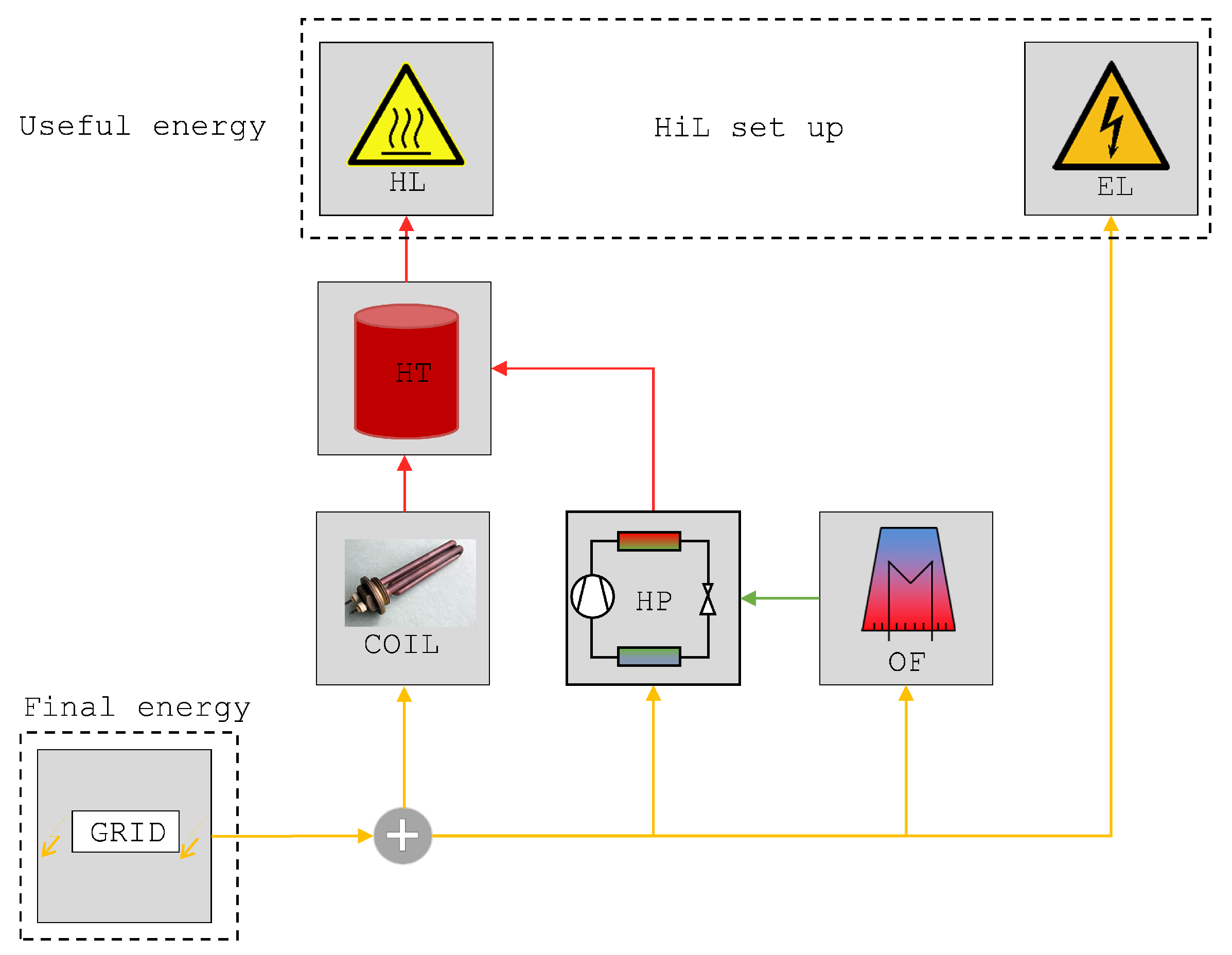
The block flow diagram of the INES system is shown in Figure 1. The low-voltage grid (GRID) supplies electricity to the air–water–electric heat pump (HP) with a heating capacity of 16 ${\mathrm{kW}}_{\mathsf{th}}$ and a nominal COP of 4.5. The outdoor fan (OF) consumes 0.9 ${\mathrm{kW}}_{\mathsf{el}}$ and is the heat source for the HP’s evaporator circuit. A mixed hot water tank (HT) with 1.5 m${}^3$ and an electrical resistance heating coil (COIL) of peak-load 6 ${\mathrm{kW}}_{\mathsf{el}}$ and 98% efficiency is also installed. The reference heating load (HL) and cooling load (CL) are emulated in a hardware-in-the-loop set-up comprising a 34 m² thermally activated test chamber with a power dissipation of 80–90 W/m² and two controllable thermostats with a heating and cooling capacity of 18 ${\mathrm{kW}}_{\mathsf{th}}$ and 10 ${\mathrm{kW}}_{\mathsf{th}}$, respectively. On the other hand, the reference electrical load (EL) profile is only used for the energy balance and cost calculations but does not have any physical effects on the hardware.

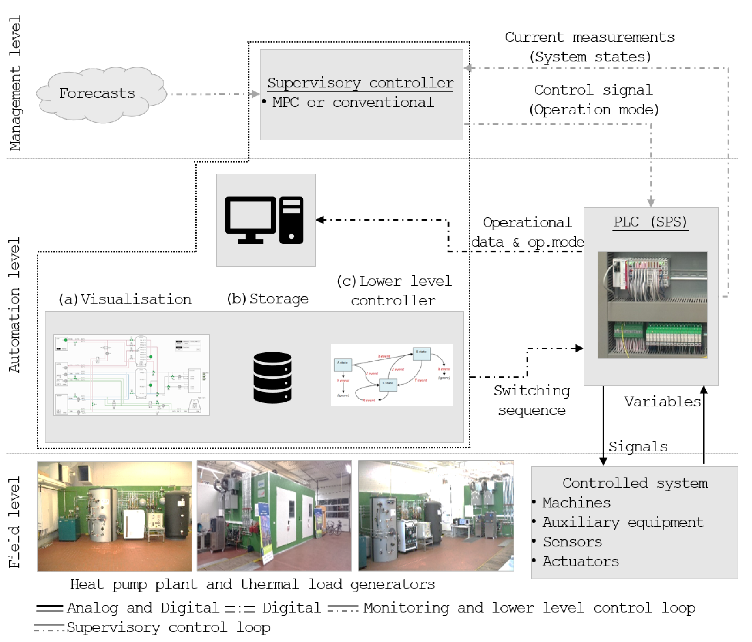
The data acquisition and control was implemented within a standard industrial BAC framework, as shown in Figure 2. Here, the supervisory controller on the management level can use either MPC or a conventional rule-based controller (for comparison purposes) to switch on the HP and/or the COIL either in parallel or alternatively. Forecasts for weather conditions and loads required by the MPC are retrieved automatically from local or remote services and databases. The management-level controller is programmed in Python and sends its control signal to the PLC (OPC server) on the automation level. A local machine (desktop computer) interacts with this server for the storing and visualization of monitoring data. Additionally, the local machine also runs a state-machine-based lower-level controller that uses the control signal (plant state) value in its sequential control logic to perform the state-based actions and transition tasks; e.g., valve sequencing or switching pumps for that particular state. The data flow represented by dash-dotted arrows uses only digital signals and standards necessary for OPC, API, and SQL communication, whereas solid arrows use both digital and analog signals; e.g., resistance and voltage and the M-Bus communication protocol. Additionally, the grey lines are part of the control loop that repeats once every control horizon, and black lines are part of the monitoring loop that repeats continuously every 300 ms.

2.2. Optimal Controller

The optimal control framework was developed based on an energy flow MIQP and implicit-MPC techniques. An economic-MPC problem, where a continuous economic cost function unifies economic optimization with process control by applying economically driven signals such as operating costs or energy costs [26], was formulated using a receding horizon scheme and physically motivated constraints for real-world applications. The following assumptions were made regarding the objective of the MPC:

• The COP of the HP is assumed constant as the focus of this work is the demonstration of the optimal control framework, and part-load efficiencies could be represented as linear curve fits without any substantial adverse effects on future formulations of the MIQP framework;
• The consumption-related costs for final energies are of more significance in an economic optimization than the operation and maintenance costs;
• If the minimum up/down time factors are included as parameters in the MPC problem, then it is redundant to include start-up and shut-down costs in the cost function;
• The tariff for final energies represents an ideal market situation in which the complex interactions between energy markets, economic and regulatory frameworks, and the status of the grid are all captured in the tariff structure.

These assumptions simplify certain highly complex issues with less significance to the end user of such control algorithms; e.g., the logic behind electricity price signals generated by grid operators or the different primary energy factors. Additionally, under the above assumptions, the cost-efficient operation of a plant could be considered supportive of the larger regional grid.

2.2.1. Models

Linear energy balance models were implemented to calculate the relevant consumption and production of components as a function of their binary control signal. For instance, the thermal capacity of the HP $P_{\mathsf{th},\mathsf{HP}}$ was calculated using (1), where $P_{\mathsf{th},\mathsf{HP},\mathsf{nom}}$ is the nominal capacity and a parameter of the heat pump model and $b_{\mathsf{HP}}\in \{0,1\}$ is its binary switch. The electrical consumption of the heat pump $P_{\mathsf{el},\mathsf{HP}}$ was calculated using (2) based on its nominal coefficient of performance $CO{P}_{\mathsf{HP}}$, also defined as a model parameter,

$$P_{\mathsf{th},\mathsf{HP}}=b_{\mathsf{HP}}{P}_{\mathsf{th},\mathsf{HP},\mathsf{nom}},$$

(1)

$$P_{\mathsf{el},\mathsf{HP}}=\frac{b_{\mathsf{HP}}{P}_{\mathsf{th},\mathsf{HP},\mathsf{nom}}}{CO{P}_{\mathsf{HP}}}.$$

(2)

Similar calculations were made for the heating capacity of the COIL $P_{\mathsf{th},\mathsf{COIL}}$ and the electrical consumption of the COIL $P_{\mathsf{el},\mathsf{COIL}}$ and of the OF $P_{\mathsf{el},\mathsf{OF}}$. For the mixed HT model, only one temperature $T_{\mathsf{HT}}$ was calculated using an ordinary differential equation based on the energy balance for the HT with a mass $m_{\mathsf{HT}}$ shown below:

$$m_{\mathsf{HT}}{c}_{\mathsf{p}}{\dot{T}}_{\mathsf{HT}}=P_{\mathsf{th},\mathsf{HP}}+P_{\mathsf{th},\mathsf{COIL}}-P_{\mathsf{th},\mathsf{HL}},$$

(3)

where HP and COIL represent the sources and the heating load $P_{\mathsf{th},\mathsf{HL}}$ generated by the HiL, which is supplied by the HT.

2.2.2. Operational Constraints

The constraints were classified as critical constraints or noncritical constraints for the simplification of the optimization problem. The violation of critical constraints leads to a solution which is not physically implementable on the plant or which leads to a system shut-down, requiring a complete manual restart. The violation of noncritical constraints does not lead to a complete manual restart, and they are included for the numerical stability of the algorithm and hardware-friendly operation. Critical constraints—e.g., the operation of HP outside the minimum permissible evaporation pressure and the maximum permissible condensation pressure of the refrigerant by using the corresponding minimum ambient temperature $T_{\mathsf{amb},\mathsf{min}}$ and maximum HT temperature $T_{\mathsf{HT},\mathsf{HP},\mathsf{max}}$, respectively—were formulated using the Big-M constraint technique [27] as shown in (4) and (5).

$$T_{\mathsf{amb}}+M(1-b_{\mathsf{HP}})\ge T_{\mathsf{amb},\mathsf{min}},$$

(4)

$$T_{\mathsf{HT}}+M(1-b_{\mathsf{HP}})\le T_{\mathsf{HP},\mathsf{max}}.$$

(5)

where $M\in {\mathbb{R}}^{+}$ is a large number chosen according to values typically expected for other variables in the equations (cf. Table 1) making the equations hold true. For instance, the application of (4) ensures that if $T_{\mathsf{amb}}<T_{\mathsf{amb},\mathsf{min}}$, and with a large M, the equation will hold true only if $b_{\mathsf{HP}}=0$. In other cases, $b_{\mathsf{HP}}$ can be 0 or 1.

The minimum runtime constraint for the HP was implemented using the following set of equations:

$$\begin{array}{c}{b}_{\mathsf{HP}}\left(t\right)-b_{\mathsf{HP}}(t+1)-Flan{k}_{\mathsf{HP}}\le 0,\end{array}$$

(6a)

$$\begin{array}{c}-b_{\mathsf{HP}}\left(t\right)+b_{\mathsf{HP}}(t+1)-Flan{k}_{\mathsf{HP}}\le 0,\end{array}$$

(6b)

$$\begin{array}{c}\sum _{\mathsf{0}}^{\mathsf{minruntime}\ast \mathsf{dt}}Flan{k}_{\mathsf{HP}}\le 1.\end{array}$$

(6c)

Here, the combination of Equations (6a) and (6b) results in the counting of $Flan{k}_{\mathsf{HP}}$, which is a binary variable that takes the value 1 every time the HP is turned on or off. Using (6c), only one flank is allowed within a user-defined HP parameter min-runtime since the sum of all $Flan{k}_{\mathsf{HP}}$ over this period, calculated as the product of minruntime and the discretization parameter $\mathrm{dt}$, should be less than 1.

Noncritical constraints—e.g., constraints on system states—as soft constraints [28] using slack variables make the numerical solution of the optimization problem more stable. For instance, the $T_{\mathsf{HT}}$ was limited within the minimum $T_{\mathsf{HT},\mathsf{min}}$ and maximum $T_{\mathsf{HT},\mathsf{max}}$ set-points as shown in (7). The violation of this constraint will not lead to the infeasibility of the optimization problem but will be penalized in the cost function.

$$T_{\mathsf{HT},\mathsf{min}}\le (T_{\mathsf{HT}}+s_{{\mathsf{T}}_{\mathsf{HT}}})\le T_{\mathsf{HT},\mathsf{max}}.$$

(7)

Finally, the electric power balance was calculated using the following equation:

$$P_{\mathsf{el},\mathsf{HP}}+P_{\mathsf{el},\mathsf{COIL}}+P_{\mathsf{el},\mathsf{OF}}=P_{\mathsf{el},\mathsf{grid},\mathsf{buy}}.$$

(8)

The simplified models and constraints form an explicit ODE system with a total number of states $n_{\mathsf{x}}=1$, number of binary controls $n_{\mathsf{b}}=2$, number of constant parameters $n_{\mathsf{p}}=12$, number of time-varying parameters $n_{\mathsf{c}}=4$ , and number of slack variables $n_{\mathsf{s}}=1$. These are given in (9a)–(9d), and the parameter set can be gathered from the model descriptions in the previously published work [29].

$$\begin{array}{c}x=\left[T_{\mathsf{HT}}\right],\end{array}$$

(9a)

$$\begin{array}{c}{b}^T=[b_{\mathsf{HP}},b_{\mathsf{COIL}}],\end{array}$$

(9b)

$$\begin{array}{c}{c}^T=[T_{\mathsf{amb}},P_{\mathsf{th},\mathsf{HL}},P_{\mathsf{el},\mathsf{EL}},r_{\mathsf{el},\mathsf{buy}},r_{\mathsf{el},\mathsf{sell}}],\end{array}$$

(9c)

$$\begin{array}{c}s=\left[s_{{\mathsf{T}}_{\mathsf{HT}}}\right].\end{array}$$

(9d)

2.2.3. Objective Function

The objective function shown in (10) finds an optimal control sequence that minimizes the consumption-related costs for electricity and penalizes violations of the soft constraints with a weight $W_{\mathsf{s}}\in {\mathbb{R}}^{n_{\mathsf{s}}\times n_{\mathsf{s}}}$,

$$\underset{x,b,s}{min}\sum _{{\mathsf{t}}_{\mathsf{o}}}^{{\mathsf{t}}_{\mathsf{f}}}\left(P_{\mathsf{el},\mathsf{grid},\mathsf{buy}}\left(t\right)r_{\mathsf{el},\mathsf{buy}}\left(t\right)+s{\left(t\right)}^T{W}_{\mathsf{s}}s\left(t\right)\right),$$

(10)

subject to, for $t\in [t_{\mathsf{0}},t_{\mathsf{f}}]$,

$$\begin{array}{c}\dot{x}\left(t\right)-f(x\left(t\right),b\left(t\right),c\left(t\right),p)=0,\end{array}$$

(11a)

$$\begin{array}{c}h\left(x\right(t),b(t),c(t),s(t),p)\le 0,\end{array}$$

(11b)

$$\begin{array}{c}x\left(t_{\mathsf{0}}\right)-x_{\mathsf{0}}=0,\end{array}$$

(11c)

$$\begin{array}{c}s\left(t\right)\ge 0,\end{array}$$

(11d)

$$\begin{array}{c}b\left(t\right)\in {\{0,1\}}^{\left\{{\mathsf{n}}_{\mathsf{b}}\right\}}.\end{array}$$

(11e)

The system dynamics and path constraints are considered in (11a) and (11b) with functions $f(·)$ and $h(·)$, respectively, while the initial state constraint is shown in (11c). The magnitude of the slack variables $s\left(t\right)$ is bounded by an upper bound value (subscript “ub”) and lower bound value (subscript “lb”). The switches of the components are the binary controls $b\left(t\right)$ that are constrained to take a value either 0 or 1 in (11e).

2.3. Conventional Controllers

Two types of conventional controllers were implemented for comparison against the MPC. The first was implemented in the experimental set-up and is based on the forbidden runtime for HP, contractually fixed by the local grid-operator. Here, the grid-operator forbids the plant-operator to run the HP at certain time frames during the day. These time frames are implemented in an if–else logic along with a conventional base load matching–following thermal load strategy. A base heating load until 10 ${\mathrm{kW}}_{\mathsf{th}}$ is satisfied by the HP alone and higher (peak) heating loads by the HP and COIL in parallel. A hysteresis dead-band logic was implemented for the individual components using the corresponding tank temperatures. The second controller is based on the FTL logic of the first controller but does not include the forbidden runtime logic, and it was implemented only in a simulation environment. The hysteresis dead-band controller is indeed the standard internal control logic often implemented by the HP manufacturers. However, the tuning of the dead-band parameters is often done during the commissioning of the HP in a non-trivial process and requires a great deal of expertise over the given system. In this study, a commercial HP of the air–water–electricity type is used, and the following thermal load controller is implemented in conjunction with the internal control logic by tuning the dead-band parameters explicitly and specifically for this plant and scenario. Hence, the MPC is indeed compared not to a standard conventional controller but to an enhanced conventional controller tuned specifically to this plant. Grey-box models that were validated against experimental data in a previous work by the authors were used for the simulation [29].

2.4. Scenario Implementation

Table 1 summarizes the parameters used to implement the scenario and set up the MPC. The load forecast is based on a residential house with an area of ca. 250 m² and peak heating load of 5.5 ${\mathrm{kW}}_{\mathsf{th}}$ and peak electrical load of 3.2 ${\mathrm{kW}}_{\mathsf{el}}$ [30]. The load profile is scaled up to match the component sizes at INES with a peak heating load of 16 ${\mathrm{kW}}_{\mathsf{th}}$ on weekends and a peak electrical load of 10.5 ${\mathrm{kW}}_{\mathsf{el}}$. A two-price tariff structure for the rate of electricity $r_{\mathsf{el},\mathsf{buy}}$ is used with a high tariff of 0.23 €/${\mathrm{kWh}}_{\mathsf{el}}$ from 07:00 to 22:00 and a lower tariff of 0.203 €/${\mathrm{kWh}}_{\mathsf{el}}$ from 22:00 to 07:00.

Table 1. Data for the time-varying parameters and constant parameters used to set up the MPC scenario.

Parameter	Data/Value	Parameter	Data/Value
For implementing the scenario:		For MPC set-up:
Ambient temperature forecast	DarkSky API for Offenburg [31]	Forecast horizon	24 h
Load forecast	Deterministic residential	Control horizon	15 min
Electricity price forecast	Two-price tariff	Optimization framework	SCIP [32]
For physical constraints:		Solver maximum CPU time	30 s
Minimum runtime of HP	1 h	Value for M in Big-M formulation	500
Maximum HT temperature for HP operation $T_{\mathsf{r},\mathsf{HP},\mathsf{H},\mathsf{max}}$	42 °C	Value for slack weights W	$1\times {10}^4$
Minimum ambient temperature for HP operation $T_{\mathsf{r},\mathsf{HP},\mathsf{H},\mathsf{min}}$	10 °C
Set feed-line temperature in test chamber heating circuit $T_{\mathsf{f},\mathsf{TC},\mathsf{set}}$	35 °C

Table 1. Data for the time-varying parameters and constant parameters used to set up the MPC scenario.

Parameter	Data/Value	Parameter	Data/Value
For implementing the scenario:		For MPC set-up:
Ambient temperature forecast	DarkSky API for Offenburg [31]	Forecast horizon	24 h
Load forecast	Deterministic residential	Control horizon	15 min
Electricity price forecast	Two-price tariff	Optimization framework	SCIP [32]
For physical constraints:		Solver maximum CPU time	30 s
Minimum runtime of HP	1 h	Value for M in Big-M formulation	500
Maximum HT temperature for HP operation $T_{\mathsf{r},\mathsf{HP},\mathsf{H},\mathsf{max}}$	42 °C	Value for slack weights W	$1\times {10}^4$
Minimum ambient temperature for HP operation $T_{\mathsf{r},\mathsf{HP},\mathsf{H},\mathsf{min}}$	10 °C
Set feed-line temperature in test chamber heating circuit $T_{\mathsf{f},\mathsf{TC},\mathsf{set}}$	35 °C

For comparison between the various controllers, the residential house profile mentioned in Section 3.1 was used to create a transition season scenario. The ambient temperature and load forecast for all controllers was similar over the entire monitoring campaign. The set-point for the feed-line to test chamber $T_{\mathsf{f},\mathsf{TC},\mathsf{set}}$ was fixed at 35 °C. The set-points for the hysteresis of the conventional controllers were selected after multiple tuning experiments and discussions with the component manufacturers specifically for the INES laboratory set-up. The time ranges required to implement the HP forbidden run-times were given in the contractual obligations of the grid-operator. All conventional control parameters are specified in

Table 2. Parameters for implementing the reference controller for summer with switching point.

Parameter	Value
$T_{\mathsf{HT},\mathsf{min}}$	38 °C
$T_{\mathsf{HT},\mathsf{max}}$	42 °C
Switching point	10 kW
HP forbidden runtimes	10:15–12:15, 17:30–18:30, 21:15–22:15

, and MPC related parameters are the same as in Table 1 specified earlier.

3. Experimental Results

A demonstration of the receding horizon MPC is given in this section, and its technical feasibility is evaluated using the results of a single MPC iteration, multiple MPC iterations, and the comparison to reference controllers, under almost-identical conditions. The duration of the test was ca. 3.5 days for each controller, whereby the ambient temperature did not vary significantly between both tests.

3.1. Single MPC Iteration

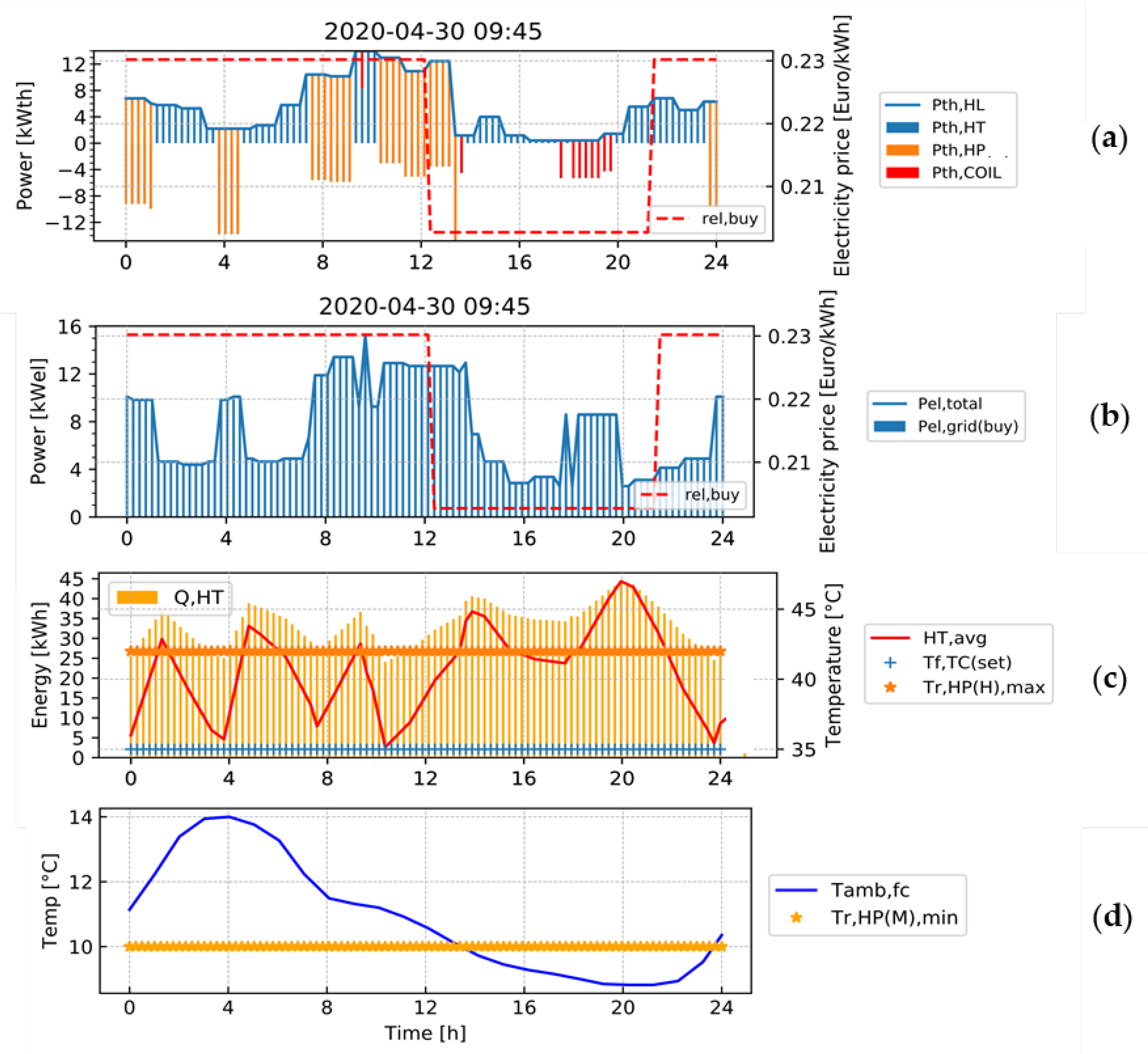
The complexity of an MPC problem arising from the interdependence of multiple inputs and outputs—e.g., ambient temperature, initial state, physical constraints, and electricity prices—is illustrated using the results of one iteration of the MPC scheme for a typical heat pump system application in the transition period.

The control signal vector from one MPC iteration comprises the switching sequence for the heat pump and the coil over the entire horizon. The resulting thermal balance, electrical balance, and tank temperatures corresponding to this binary control signal are shown in Figure 3a–c. The ambient temperature forecast over the horizon is shown in Figure 3d. The following significant observations are made:

Grid-supportive operation of MPC: Considering the assumption that the electricity price structure reflects the grid’s status in terms of consumption and generation profiles and grid congestion, the economic-MPC operates the plant in a grid-supportive manner wherein (i) the switching of the components is reactive to the electricity price, (ii) the storages are charged predictively to support peak thermal loads, and (iii) longer duration of peak loads are avoided. For instance, as seen in the thermal balance in Figure 3a, the HP operation is preferred in times of higher electricity price $r_{\mathsf{el},\mathsf{buy}}$ with its thermal capacity $P_{\mathsf{th},\mathsf{HP}}$ covering the heating load $P_{\mathsf{th},\mathsf{HL}}$ and excess energy (negative values) stored in the tank. As expected, this leads to a rise in the tank’s temperature $H{T}_{\mathsf{avg}}$ and energy $Q_{\mathsf{HT}}$, as seen in Figure 3c. On the other hand, the COIL operation $P_{\mathsf{th},\mathsf{COIL}}$ is reduced in these times. It is instead operated during lower $P_{\mathsf{th},\mathsf{HL}}$ and lower $r_{\mathsf{el},\mathsf{buy}}$ at night to charge the HT predictively to support the forecasted peak loads of the next day. Such an operation leads to shorter peaks in the total electrical requirement $P_{\mathsf{el},\mathsf{total}}$, especially in times of higher $r_{\mathsf{el},\mathsf{buy}}$ as seen in the corresponding electrical balance in Figure 3b. Since the system has no possibility to produce electricity, the $P_{\mathsf{el},\mathsf{total}}$ is completely satisfied by purchasing electricity from the grid $P_{\mathsf{el},\mathsf{grid},\mathsf{buy}}$. It is observed that longer HP operation during the day for the charging of the HT does not occur, and HP operation during the night is also avoided. These patterns are clarified in the next point on the operational constraints.

MPC finds an optimal state vector while respecting operational constraints: The optimal solution for switches of the heat pump maintains a minimum run time of 1 h. However, a longer operation is avoided in certain cases as the $H{T}_{\mathsf{avg}}$ increases beyond the $T_{\mathsf{r},\mathsf{HP},\mathsf{H},\mathsf{max}}$ and the HP is turned off as shown in Figure 3c. Additionally, it is seen that the optimal solution maintains the $H{T}_{\mathsf{avg}}$ (system state) to be always higher than the set-point temperature for the heating feed-line circuit $T_{\mathsf{f},\mathsf{TC},\mathsf{set}}$. Hence, an adequate temperature for the heating circuit is always provided. Similarly, it is observed in Figure 3d that HP is not operated in times in which the ambient temperature is lower than the minimum limit set for HP operation $T_{\mathsf{r},\mathsf{HP},\mathsf{M},\mathsf{min}}$. This is in accordance with the operational constraints formulated in the optimization problem.

The morning and afternoon peaks in the forecasted load are in accordance with a typical residential load profile. It is clear here that with MPC, multiple aspects of the plant’s operation are covered. However, one of the core advantages of this controller is the update of the forecast, and this is observed in the next section with results from multiple MPC iterations.

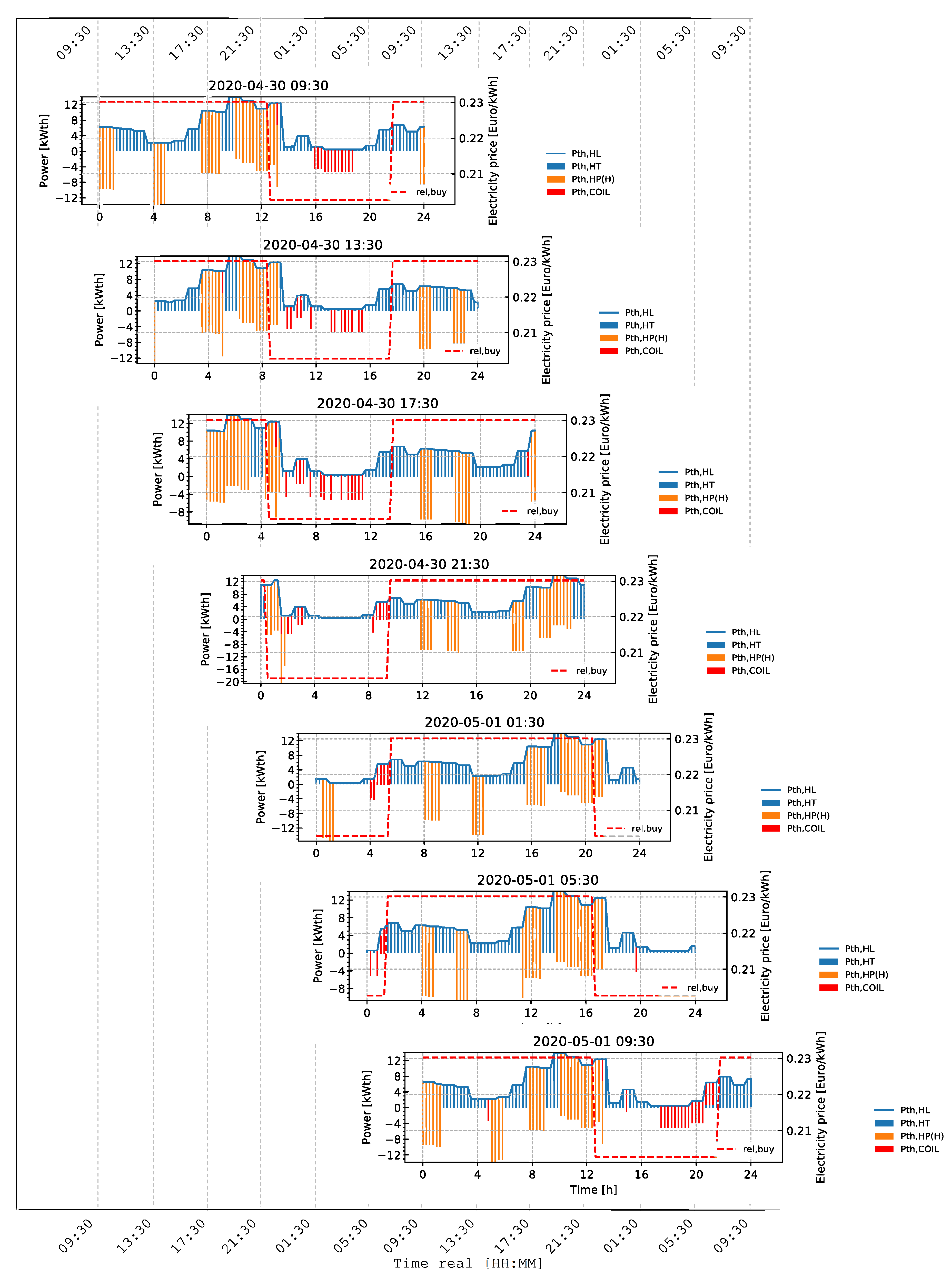
3.2. Multiple MPC Iterations

As an example of the receding horizon scheme, multiple MPC iterations during a 24 h experiment with the same parameters as in Table 1 were collected. The thermal balance for an iteration after every 4 h is illustrated as a subplot in Figure 4. As the forecast horizon recedes or shifts, the heating load forecast $P_{\mathsf{th},\mathsf{HL}}$ and electricity price $r_{\mathsf{el},\mathsf{buy}}$ for the next 24 h are updated and a new optimal schedule is calculated. For instance, in the second subplot (2020-04-30 13:30) the $P_{\mathsf{th},\mathsf{HP},\mathsf{H}}$ between Time = 0 h to 4 h is different compared to the solution in the first subplot (2020-04-30 09:30). Thus, the actual solution applied on the plant was more adjusted to the current situation of the plant and the grid. Additionally, the forecasted operation of the COIL also differed in all the subplots due to the update of the forecast data.

The computation time for an iteration was often between 3 to 5 s. This was considerably shorter than the control horizon and facilitated the usage of most recent plant data at each iteration. Since only the first element from the MPC’s solution vector was applied to the plant, it was not possible to determine without monitoring data how the real operation occurred. Hence, it is of paramount importance to have such data from experiments, especially for a comparison with conventional controllers. Results from such an experiment are presented in the next section.

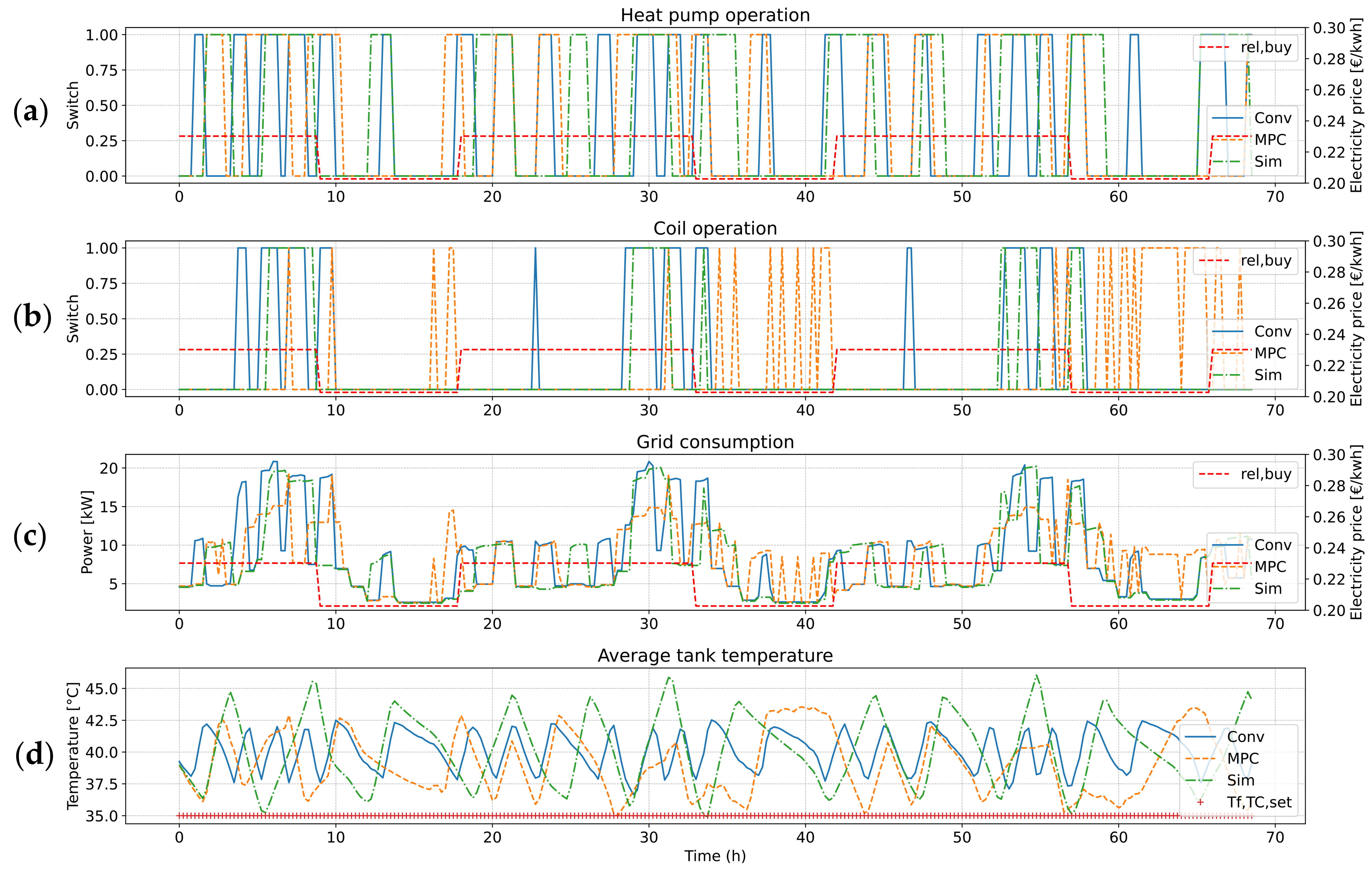
3.3. Comparison of Conventional Controllers and MPC

The forbidden runtime controller and MPC were each tested for ca. 68 h, and the FTL conventional controller was simulated for the same time. All controllers started with similar initial tank temperatures. To understand the fundamental differences in the actions of the controllers, the switching sequences and electrical balance along with the electricity price are plotted in Figure 5a–c. Additionally, as an example of the physical constraints, the average tank temperature for the three controllers is plotted in Figure 5d. The results of the test with a conventional forbidden runtime controller are plotted in blue (Conv), with MPC in orange (MPC), and with the simulated FTL controller in green (Sim). The significant observations are summarized below.

Grid-adverse operation of conventional controllers and grid-supportive operation of MPC: Interpreting the switching patterns in Figure 5a,b with respect to the electricity price $r_{\mathsf{el},\mathsf{buy}}$, it is observed that the conventional controllers operated the HP and the COIL for longer and more often than the MPC during the day. This behavior was more frequent when high thermal and electrical loads occurred simultaneously and was significantly grid-adverse since electrical peaks (see Figure 5c) were generated during times of high $r_{\mathsf{el},\mathsf{buy}}$. On the other hand, the MPC predictively charged the HT (almost until maximum permissible temperatures for HP operation) by operating the COIL at night time with lower tariff.

Simpler tuning of MPC: The tuning of the MPC was done by defining the permissible operation range in the HT using the parameters $T_{\mathsf{HT},\mathsf{max}}$ and $T_{\mathsf{HT},\mathsf{min}}$, which corresponds to $T_{\mathsf{f},\mathsf{TC},\mathsf{set}}$. The operation was further bounded with temperature limits $T_{\mathsf{r},\mathsf{HP},\mathsf{H},\mathsf{max}}$ and $T_{\mathsf{r},\mathsf{HP},\mathsf{M},\mathsf{min}}$, which were promptly defined in datasheets of the components. These constraints specified a wide operational range. As discussed in Section 3.1, the MPC automatically found an optimal solution within this range, whereas the tuning of the reference controllers was a non-trivial process of commissioning routines, simulation studies, or guesswork based on the recommendation of individual component manufacturers (often not directly suitable for multicomponent systems).

Hysteresis control is noticed for conventional controllers: In Figure 5d, the FTL strategy using hysteresis control over the tank temperature is observed for the both conventional controllers. The HP is activated when the tank temperature is cooler than $T_{\mathsf{HT},\mathsf{min}}$ and remains active until the tank temperature is hotter than $T_{\mathsf{HT},\mathsf{max}}$. This operation gives the hysteresis controller its distinct saw-tooth pattern.

MPC did not violate minimum runtime constraint: The heat pump was operated at least for 1 h by the MPC as specified in its minimum runtime constraint. However, since this constraint was not implemented as a hard rule in the conventional controllers, it sometimes operated for less than 1 h. Either this restriction must be programmed in the if–else logic of the conventional controller or implemented over the tuning of the hysteresis temperatures. Executing any of these will be non-trivial compared to the simple tuning of the MPC.

Adequate heating feed-line temperature in HT: All controllers were able to maintain an adequate heating temperature in the HT above $T_{\mathsf{f},\mathsf{TC},\mathsf{set}}=35$ °C. Nevertheless, the MPC uses the tank capacity optimally with the average tank temperature often reaching the minimum limit of 35 °C. Especially at the end of experiment, the predictive nature of MPC control uses the tank energy completely and finishes with a tank temperature of ca. 35 °C.

An economic analysis of the experimental data from the first conventional controller and MPC and simulation data of the second conventional controller showed a small saving of ca. 1.5% in the consumption-related costs with MPC over the conventional controllers. However, it must be taken into account that the forbidden runtime from the grid operator was not part of the MPC framework, and to draw definite conclusions, further testing will be necessary. An operational analysis of the measured data (similar to Figure 3d) revealed that MPC did not violate the minimum ambient temperature and maximum hot tank temperature conditions for HP operation. The conventional controller, however, violated this constraint by operating the heat pump even though $T_{\mathsf{amb}}$ was lower than the restricted value of 10 °C. More experiments and simulations with various load profiles and component sizes will be necessary to quantify the benefits with high certainty. This is planned in the near future.

4. Discussion

The analysis of single and multiple MPC iterations in Section 3.1 and Section 3.2 established the technical feasibility of MPC to provide a predictive switching schedule capable of considering multiple input forecasts, hardware constraints, and storage capacities simultaneously. Additionally, the process of a receding horizon scheme was displayed. However, for the development of the component models and interpretation of the results, significant domain knowledge was necessary.

The linear models provided fast solutions and were directly implementable in a MIQP framework but could not capture the complex part-load behaviors of the heat pump. Similarly, the implementation of a simple two-tariff electricity price structure did not help to demonstrate the complete advantage of the MPC scheme, which would be achieved with complex real-time dynamic pricing. These factors should be included in the further development of the MPC framework.

The grid-friendly operation of the suggested MPC was only valid under the circumstance that the electricity price signal captured all features of the grid and incentivized the production or consumption of electricity at relevant time frames. Thus, in its current form, with a 15 min control horizon and working with slower thermal systems, the optimization may not be able to participate in faster markets such as primary reserve control or secondary reserve control. A significant question still to be answered would be the ability of the hardware to react to this volatility and choice of control horizon. However, if a signal from the energy market in the future provides for these challenges and allows slower thermal systems to intelligently interact with the market without rebound effects, then the optimal control framework proposed in this study could be a practical approach.

Finally, the MPC was also compared under almost-identical circumstances with two different conventional controllers: firstly, a conventional controller implementing both the following thermal load-base load matching strategy and the forbidden runtime for HP as per the grid-operator’s contract, and secondly, an exclusive FTL conventional controller. No significant economic benefits were seen in the MPC due to a strong dependence on the type of profile and controller tuning parameters. For instance, the conventional controllers were specifically tuned for the INES heat pump plant and may be considered as enhanced conventional controllers that are difficult to beat in this scenario. Nonetheless, an operational constraint on minimum ambient temperature for the heat pump was violated by the reference controller since it was not part of its hard-coded logic. Either the code must be adjusted or, with further commissioning tests and calculations or simulations, the control logic of the system would need to be adapted. Moreover, such a tuning may be effective only for the target scenario, and the performance of the reference controller may deteriorate outside the tuning range, making it difficult to adapt for other systems.

5. Conclusions and Outlook

The potential of MPC for operating complex energy systems in a coordinated network and supporting the energy grid of the future is expressed in previous theoretical studies, and this work demonstrated its viability and usefulness in a practical environment. Theoretical concepts of mixed integer quadratic programming and the practical framework of a building automation and control system were integrated together to demonstrate the application of an economic-MPC approach for the optimal scheduling of a model heat pump plant with standard industrial components at the INES polygeneration lab. Technical advantages of MPC that were also reported in the literature—e.g., easier tuning and extension of existing framework, grid-supportive scheduling of the components, and lower constraint violations—were experimentally verified.

The majority of the workload for setting up the MPC was in the modeling efforts. No significant economic benefits could be found, and they were lower than the range reported in literature. However, since the magnitude of benefits is strongly dependent on various factors such as the load profile and initialization parameters of the MPC, it will be necessary to perform further extensive tests both as lab experiments and simulations to quantify the benefits. One immediate way to proceed would be to implement the high-accuracy plant model as a digital-twin for the MPC solver and simulate longer test periods. Additionally, in the near future, it is planned to implement real-time pricing signals in the optimization framework to demonstrate further the advantages of MPC. Another exciting possibility for research could be to implement machine learning algorithms to develop the control-oriented component models in order to reduce the modeling efforts in deploying the MPC.

References

- Bundesverband Wärmepumpe (BWP) e.V. Marktanalyse—Szenarien—Handlungsempfehlungen. 2021. Available online: www.waermepumpe.de (accessed on 29 September 2021).
- Al Moussawi, H.; Fardoun, F.; Louahlia-Gualous, H. Review of tri-generation technologies: Design evaluation, optimization, decision-making, and selection approach. Energy Convers. Manag. 2016, 120, 157–196. [Google Scholar] [CrossRef]
- Fischer, D.; Madani, H. On heat pumps in smart grids: A review. Renew. Sustain. Energy Rev. 2017, 70, 342–357. [Google Scholar] [CrossRef] [Green Version]
- Drgoňa, J.; Arroyo, J.; Figueroa, I.C.; Blum, D.; Arendt, K.; Kim, D.; Ollé, E.P.; Oravec, J.; Wetter, M.; Vrabie, D.L.; et al. All you need to know about model predictive control for buildings. Annu. Rev. Control 2020, 50, 190–232. [Google Scholar] [CrossRef]
- Serale, G.; Fiorentini, M.; Capozzoli, A.; Bernardini, D.; Bemporad, A. Model predictive control (MPC) for enhancing building and HVAC system energy efficiency: Problem formulation, applications and opportunities. Energies 2018, 11, 631. [Google Scholar] [CrossRef] [Green Version]
- Kim, J.S.; Edgar, T.F. Optimal scheduling of combined heat and power plants using mixed-integer nonlinear programming. Energy 2014, 77, 675–690. [Google Scholar] [CrossRef]
- Liu, P.; Georgiadis, M.C.; Pistikopoulos, E.N. An energy systems engineering approach for the design and operation of microgrids in residential applications. Chem. Eng. Res. Des. 2013, 91, 2054–2069. [Google Scholar] [CrossRef]
- Facci, A.L.; Andreassi, L.; Ubertini, S. Optimization of CHCP (combined heat power and cooling) systems operation strategy using dynamic programming. Energy 2014, 66, 387–400. [Google Scholar] [CrossRef]
- Liu, M.; Shi, Y.; Fang, F. Combined cooling, heating and power systems: A survey. Renew. Sustain. Energy Rev. 2014, 35, 1–22. [Google Scholar] [CrossRef]
- Ortiga, J.; Bruno, J.C.; Coronas, A. Operational optimisation of a complex trigeneration system connected to a district heating and cooling network. Appl. Therm. Eng. 2013, 50, 1536–1542. [Google Scholar] [CrossRef]
- Bürger, A.; Bohlayer, M.; Hoffmann, S.; Altmann-Dieses, A.; Braun, M.; Diehl, M. A whole-year simulation study on nonlinear mixed-integer model predictive control for a thermal energy supply system with multi-use components. Appl. Energy 2020, 258, 114064. [Google Scholar] [CrossRef] [Green Version]
- Fischer, D.; Bernhardt, J.; Madani, H.; Wittwer, C. Comparison of control approaches for variable speed air source heat pumps considering time variable electricity prices and PV. Appl. Energy 2017, 204, 93–105. [Google Scholar] [CrossRef]
- Zwickel, P.; Engelmann, A.; Gröll, L.; Hagenmeyer, V.; Sauer, D.; Faulwasser, T. A Comparison of Economic MPC Formulations for Thermal Building Control. In Proceedings of the 2019 IEEE PES Innovative Smart Grid Technologies Europe (ISGT-Europe), Bucharest, Romania, 29 September–2 October 2019; pp. 1–5. [Google Scholar] [CrossRef]
- Oldewurtel, F.; Parisio, A.; Jones, C.N.; Gyalistras, D.; Gwerder, M.; Stauch, V.; Lehmann, B.; Morari, M. Use of model predictive control and weather forecasts for energy efficient building climate control. Energy Build. 2012, 45, 15–27. [Google Scholar] [CrossRef] [Green Version]
- Thieblemont, H.; Haghighat, F.; Ooka, R.; Moreau, A. Predictive control strategies based on weather forecast in buildings with energy storage system: A review of the state-of-the art. Energy Build. 2017, 153, 485–500. [Google Scholar] [CrossRef] [Green Version]
- Franco, A.; Miserocchi, L.; Testi, D. Energy Intensity Reduction in Large-Scale Non-Residential Buildings by Dynamic Control of HVAC with Heat Pumps. Energies 2021, 14, 3878. [Google Scholar] [CrossRef]
- Kuboth, S.; Weith, T.; Heberle, F.; Welzl, M.; Brüggemann, D. Experimental Long-Term Investigation of Model Predictive Heat Pump Control in Residential Buildings with Photovoltaic Power Generation. Energies 2020, 13, 6016. [Google Scholar] [CrossRef]
- Rastegarpour, S.; Caseri, L.; Ferrarini, L.; Gehrke, O. Experimental validation of the control-oriented model of heat pumps for MPC applications. In Proceedings of the 2019 IEEE 15th International Conference on Automation Science and Engineering (CASE), Vancouver, BC, Canada, 22–26 August 2019; pp. 1249–1255. [Google Scholar]
- Péan, T.Q.; Salom, J.; Costa-Castelló, R. Review of control strategies for improving the energy flexibility provided by heat pump systems in buildings. J. Process. Control 2019, 74, 35–49. [Google Scholar] [CrossRef]
- Váňa, Z.; Cigler, J.; Široký, J.; Žáčeková, E.; Ferkl, L. Model-based energy efficient control applied to an office building. J. Process. Control 2014, 24, 790–797. [Google Scholar] [CrossRef]
- Sturzenegger, D.; Gyalistras, D.; Gwerder, M.; Sagerschnig, C.; Morari, M.; Smith, R.S. Model Predictive Control of a Swiss office building. In Proceedings of the Clima-Rheva World Congress, Prague, Czech Republic, 16–19 June 2013; pp. 3227–3236. [Google Scholar]
- Ma, J.; Qin, S.J.; Salsbury, T. Application of economic MPC to the energy and demand minimization of a commercial building. J. Process. Control 2014, 24, 1282–1291. [Google Scholar] [CrossRef]
- Afram, A.; Janabi-Sharifi, F. Supervisory model predictive controller (MPC) for residential HVAC systems: Implementation and experimentation on archetype sustainable house in Toronto. Energy Build. 2017, 154, 268–282. [Google Scholar] [CrossRef]
- Dittmann, A.; Kober, P.; Lorenz, E.; Villegas Mier, O.; Ruf, H.; Schmidt, M. Optimierung der PV-Speisung von Wärmepumpen Durch Kurzfristprognosen mit Wolkenkameras. In Proceedings of the PV Symposium, Bad Staffelstein, Germany, 19–21 March 2019. [Google Scholar]
- Sawant, P. A Contribution to Optimal Scheduling of Real-World Trigeneration Systems Using Economic Model Predictive Control; Technische Universität Dresden: Dresden, Germany, 2021; Available online: https://www.shaker.de/de/content/catalogue/index.asp?lang=de&ID=8&ISBN=978-3-8440-8055-1&search=yes (accessed on 29 September 2021).
- Ellis, M.; Durand, H.; Christofides, P.D. A tutorial review of economic model predictive control methods. J. Process. Control 2014, 24, 1156–1178. [Google Scholar] [CrossRef]
- Griva, I.; Nash, S.G.; Sofer, A. Linear and Nonlinear Optimization; SIAM: Philadelphia, PA, USA, 2009; Volume 108. [Google Scholar]
- Lefort, A.; Bourdais, R.; Ansanay-Alex, G.; Guéguen, H. Hierarchical control method applied to energy management of a residential house. Energy Build. 2013, 64, 53–61. [Google Scholar] [CrossRef]
- Sawant, P.; Bürger, A.; Doan, M.D.; Felsmann, C.; Pfafferott, J. Development and experimental evaluation of grey-box models of a microscale polygeneration system for application in optimal control. Energy Build. 2020, 215, 109725. [Google Scholar] [CrossRef]
- Ren, H.; Gao, W.; Ruan, Y. Optimal sizing for residential CHP system. Appl. Therm. Eng. 2008, 28, 514–523. [Google Scholar] [CrossRef]
- Kubis, L. Darksky API for Python: Darkskylib. 2018. Available online: https://github.com/lukaskubis/darkskylib (accessed on 20 August 2019).
- Gamrath, G.; Anderson, D.; Bestuzheva, K.; Chen, W.K.; Eifler, L.; Gasse, M.; Gemander, P.; Gleixner, A.; Gottwald, L.; Halbig, K.; et al. The Scip Optimization Suite 7.0. 2020. Available online: http://nbn-resolving.de/urn:nbn:de:0297-zib-78023 (accessed on 29 September 2021).
Figure 1.
Block flow diagram of the heat pump-based building energy system. HP (heat pump), COIL (heating coil), HiL (hardware in the loop), HT (hot tank), HL (heating load), EL (electrical load), OF (outdoor fan).
Figure 2.
Building automation and control framework of the INES plant. Dash-dotted arrows represent only digital signals, whereas solid arrows represent analog and digital signals. Grey lines are part of the control loop, and black lines are part of the monitoring loop. The supervisory controller on the management level and the storage of data, its visualization, and a state-machine lower-level controller on the automation level are operated on the same local machine, represented as the box with dotted line.
Figure 3.
Graphical representation and feasibility check of the MPC’s solution at 09:45 (Time = 0 h) for a 24 h forecast horizon for a test in transition season. (a) Thermal balance, (b) electrical balance, (c) tank energy and temperature, and (d) ambient temperature forecast. Negative represents charging of HT.
Figure 4.
Multiple MPC iterations in 4 h intervals representing a 24 h test. The shifting of the horizon and updates of the forecast, electricity rate, and optimal schedule are noticed in each sub-plot; for instance, the inclusion of more HP operations during the cheaper electricity rate as a higher heating load is forecasted on the horizon.
Figure 5.
Experimental and simulation data for the three controllers with respect to (Top to bottom) (a) heat pump operation, (b) coil operation, (c) grid consumption, (d) average tank temperature.