Article

Numerical Study on the Effect of the Pipe Groove Height and Pitch on the Flow Characteristics of Corrugated Pipe

1
School of Mechanical, Automotive and Aeronautical Engineering, Korea National University of Transportaion, Chungju-si 27469, Korea
2
School of Mechanical System Engineering, Chung-Ang University, Seoul 06974, Korea
3
Fire Insurers Laboratories of Korea, Yeoju-si 12661, Korea
4
Big Anvil Co. Ltd., Yongin-si 17128, Korea
*
Author to whom correspondence should be addressed.
Submission received: 10 February 2021 / Revised: 25 April 2021 / Accepted: 28 April 2021 / Published: 2 May 2021
(This article belongs to the Special Issue Computational Fluid Dynamics (CFD) 2021)

Abstract

:
For corrugated pipes with a square groove, it is known that there is no interaction between the main flow and groove flow when the aspect ratio is less than four. When the groove length and height are different, the interaction occurs in the pipe. In previous studies, it was investigated whether this interaction is dependent on groove length. However, when changing the groove height, the shape of the vortex generated inside the groove changes, which may cause the interaction to occur. Therefore, in this paper the interaction between the main and groove flow of corrugated pipes is investigated when changing both groove height as well as groove pitch, corresponding to an aspect ratio of less than four. For the groove height, the flow out of the groove after impingement changes with the shape of the secondary vortex in the groove. This flow deforms the velocity distribution in the main flow, and thus the friction factor is different. For the groove pitch, there is no difference in v-velocity distribution at the interface at the 5th and 20th groove. This means there is no interaction between the grooves, and, the friction factor differs as the number of grooves differs.

1. Introduction

Pipes play an essential role in transferring energy and fluid in a wide range of settings including fire industries, power plants, plumbing, and buildings. Generally, smooth pipes are used in large-scale facilities where there are no space constraints. However, where space is restricted, fire or disaster site, the smooth pipe is unsuitable, and flexible corrugated pipe is used a lot. The advantage of being able to transfer heat more effectively than an ordinary smooth pipe by virtue of its corrugated shape.
Typically, particles that make-up a fluid will follow a smooth path without interrupting each other. However, where smooth flow is interrupted, such as in the vicinity of the groove in corrugated pipes, a small swirl area occurs, resulting in changing laminar flow to turbulence flow. This turbulence prevents viscous substances adhering to the pipe wall and effectively delivers energy from various industrial fields. Then, in terms of geometric characteristics, corrugated pipe with a wide cross-sectional area exhibits higher performance than the smooth pipe. Furthermore, corrugated pipe plays important role in withstanding hazardous settings because of the endurability, flexibility, and elasticity of the pipe itself, and in transferring a great deal of energy by virtue of its geometric make-up. Owing to the many advantages of corrugated pipes, they are widely used in heat exchangers and many industrial fields. However, the geometric make-up of the corrugated pipe causes vortexes inside the groove, resulting in other problems that can trigger complex flow phenomena inside the pipe. García et al. [1] confirmed that the transition from laminar flow to turbulent flow occurred rapidly due to the groove shape of the wall. Unal et al. [2] conducted a study on a corrugated channel with continuous grooves for turbulent flow; the unstable vortex inside the groove affects the bulk flow and subsequent grooves, which significantly increases the Reynolds stress. Popiel et al. [3] investigated friction factor for a corrugated pipe with a U-shaped groove, and an experiment was conducted up to a Reynolds number of 30,000. As the height and pitch of the groove decreased, the friction factor decreased, and as the Reynolds number increased, the friction factor increased. Similarly, Bernhard et al. [4] conducted an experiment with a Reynolds number of up to 100,000 using a U-shaped groove. The friction factor did not change significantly until the Reynolds number is 40,000, but increased when the Reynolds number exceeded 40,000. This is because the main flow goes into the groove at the Reynolds number 40,000 and above. Smith et al. [5], analyzed the flow of a channel with a square groove using numerical analysis; due to the recirculation flow inside the groove, skin friction increases at the groove top, which increases friction loss. The purpose of the many grooves in such corrugated pipes is to allow for the possibility of increasing the friction factor pertaining to decreasing energy transport, which is related to the shape of the pipe, length, and grooves. On account of geometric conditions, it is difficult to predict the pressure loss generated by the fluid’s viscosity near the pipe or duct surface within the corrugated pipe itself. Corrugated pipes are mainly composed of grooves of various shapes, but as mentioned above, many studies have been conducted in the case of U-shaped grooves. However, the corrugated pipe usually has square shapes. For corrugated pipes with square grooves, and a variety of geometric parameters including groove height, the pitch between grooves, and the length of the groove, have a significant effect on the flow characteristics of the pipes.
Perry et al. [6] classified the square shape grooves into two types based on the groove’s length and height; type-k and type-d. In the case of type-k, this refers to the pipe where the groove length is greater than the groove height. In this case, the main flow enters the groove and interacts with it, since the vortex inside the groove only occurs in the groove’s corner. Conversely, type-d refers to pipes in which the length of the groove is less than its height, meaning that the main stream cannot penetrate the groove, since the vortex fills the groove so that no interaction can occur. Tani [7] proposed a classification based on the groove’s aspect ratio and suggested that if the aspect ratio is lower than four, it can be treated separately without interaction between the main flow and the groove flow. Vijiapurapu et al. [8] analyzed the square groove for the corrugated pipes, and proposed to classify the criterion of flow interaction as the ratio of groove pitch to height. It was suggested that there is no interaction when the ratio of the groove pitch to height is less than five. However, Djenidi et al. [9] analyzed turbulent flow in a plate with a groove aspect ratio of less than four using a laser, and, even in this case, a strong ejection from the groove to the main flow was observed. Stel et al. [10] analyzed the flow in a corrugated pipe which had a groove shape that covered all of the above ranges. Since part of the main flow crosses the boundary and enters the groove, this flow squeezes the vortex inside the groove and affects the downstream part of the corner. In addition, the flow of the downstream portion of the groove impacts the corner of the groove, and some of it flows out of the groove. These flows increase turbulent kinetic energy and Reynolds stress in the downstream portion of the groove, and thus friction factor also increases. This effect depends on groove length. It was shown that interaction existed even when the aspect ratio was less than four, and Stel et al. [11] concluded that the radius of the internal vortex’s rotation increases, and the shape of the vortex in the groove changes according to the change in the height of the groove. This change of vortex caused a change in v-velocity at the groove and main flow boundary. Furthermore, the change of v-velocity generated shear at the interface, affecting turbulent kinetic energy and pressure. Therefore, it affects the main flow, and this changes the friction factor. However, most research to date has been conducted on groove length, but research conducted on groove height is insufficient.
Previous studies have been conducted where only the groove geometry is changed, however as the groove pitch decreases, the flow from the groove can enter the next groove, and there may be interactions between the grooves. To analyze these effects, we investigated the flow characteristics while decreasing the groove pitch.
Vijiapurapu et al. [12] compared four different turbulence models for the corrugated pipe with the rectangular groove, which are the Large Eddy Simulation (LES), the Reynolds Stress Model (RSM), the k-ω SST model, and the standard k-ε model, for square groove corrugated pipes with a Reynolds number range of 50,000 to 100,000. It was suggested that all four models could produce satisfactory results.
Many prior studies consider the flow of corrugated pipes, but studies on the effects of groove height and pitch on flow characteristics are insufficient. Thus, the effect of the groove height and pitch on flow characteristics has been investigated by using a numerical method when the aspect ratio was less than four. In this study, the standard k-ε model and the wall function were applied, and an experiment using a smooth pipe was also conducted to validate the numerical friction factor. In addition, to justify using a k-ε model we compared our velocity distribution in the corrugated pipe with the velocity distribution of Vijiapurapu et al. [12]

2. Numerical Study

2.1. The Govering Equations

Numerical analysis has been conducted using commercial package ANSYS Fluent to analyze the effect of the groove height and pitch on the flow characteristics of the corrugated pipe. The governing equations for steady incompressible flow was used as follows [13]:
  • Mass conservation equation
    ρ x i ( u i ) = 0
  • Momentum equation
    ρ x j ( u i u j ) = p x i + x j [ μ ( u i x j + u j x i 2 3 δ i j u l x l ) ] + ρ x j ( u i u j ¯ )
  • Turbulence energy equation
    ρ u i k x i = σ i j u j x i ρ ε + x i [ ( μ + μ t σ k ) k x i ]
  • Turbulence dissipation equation
    ρ u i ε x i = C ε 1 ε k σ i j u j x i C ε 2 ρ ε 2 k + x i [ ( μ + μ t σ k ) ε x i ]
  • Turbulence viscosity
    μ t = ρ C μ k 2 ε
    where ρ is the fluid density, μ is the dynamic viscosity, ui is components of the velocity vector, k is turbulence kinetic energy, ε is turbulence dissipation rate, and σij is the Reynolds stress tensor.

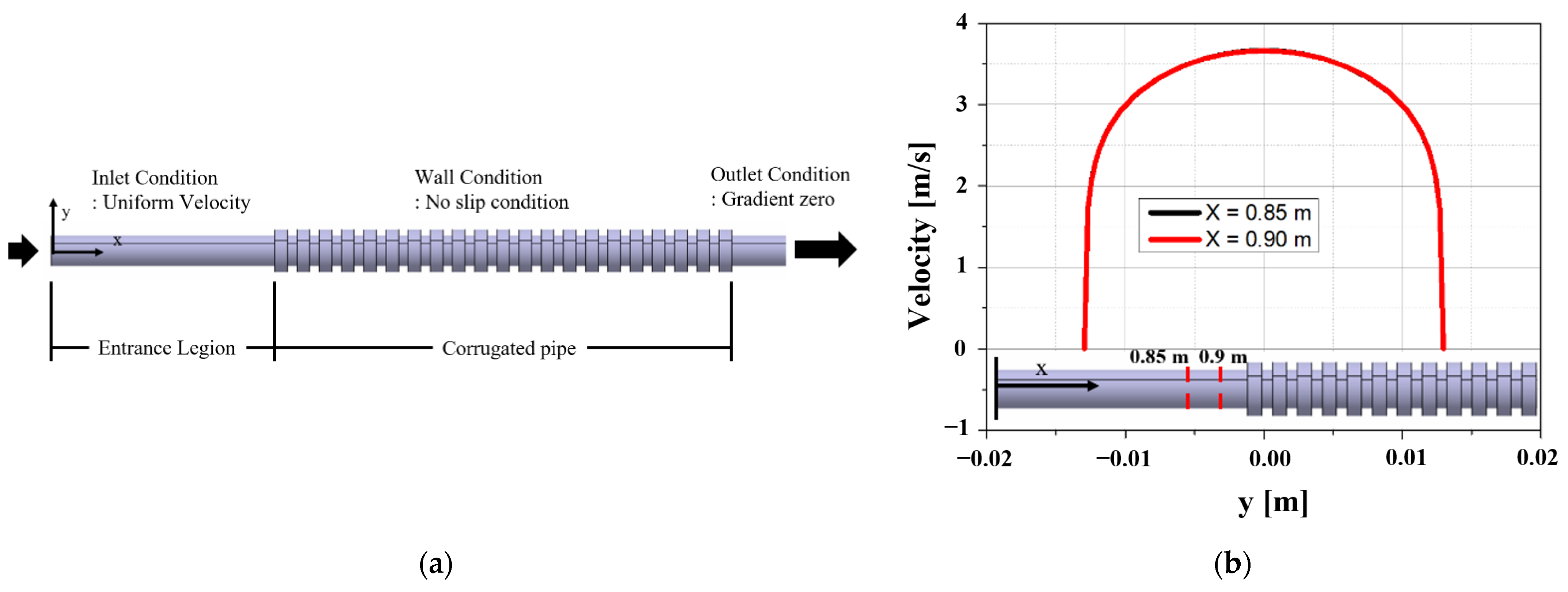
2.2. Computaional Domain and Boundary Conditions

When it comes to analyzing the effect of the corrugated pipe, the flow in the pipe should be a fully developed flow. In order to implement a fully developed flow, a computational domain of pipe was extended to the inlet length Le from the corrugated pipe. The inlet length Le was chosen by the following equation:
L e D = 4.4 ( R e ) 1 6 ,   for   Turbulent
where Le is the length of the entrance region, D is the inner pipe diameter, and Re is the Reynolds number.
Figure 1 and Table 1 represent geometrics and parameters of the corrugated pipe for this study, where w is the groove length, K is the groove height, P is the groove pitch, and s is the distance between the grooves. Cases 1 to 3 are for the effects of groove height, and Cases 3 to 5 are for the effects of groove pitch.
Since the inlet condition is given as uniform velocity, it is necessary to check whether the flows are fully developed before entering the corrugated pipe. The velocity distribution was compared at 0.85 m and 0.9 m in the x-direction from the pipe inlet. Figure 2 shows that the velocity distributions are no different. Thus, the fully developed flow is confirmed. Figure 2 contains the information on the boundary conditions of the corrugated pipe. The wall no-slip condition on the wall is applied. Since corrugated pipes are mainly used for pipe connection, zero gradients conditions are set at the outlet. The SIMPLE algorithm was used to solve the pressure and velocity coupling problem, and convergence judgment was set to 10−4 as the residual.

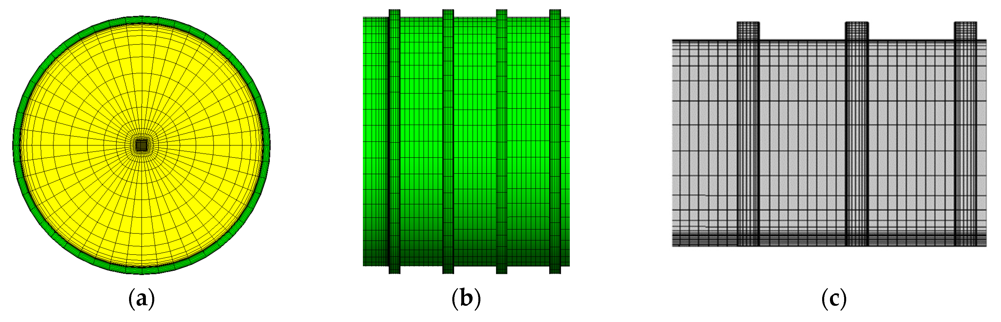
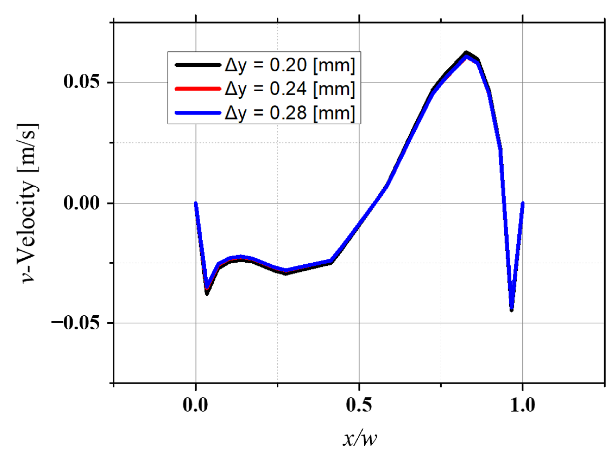
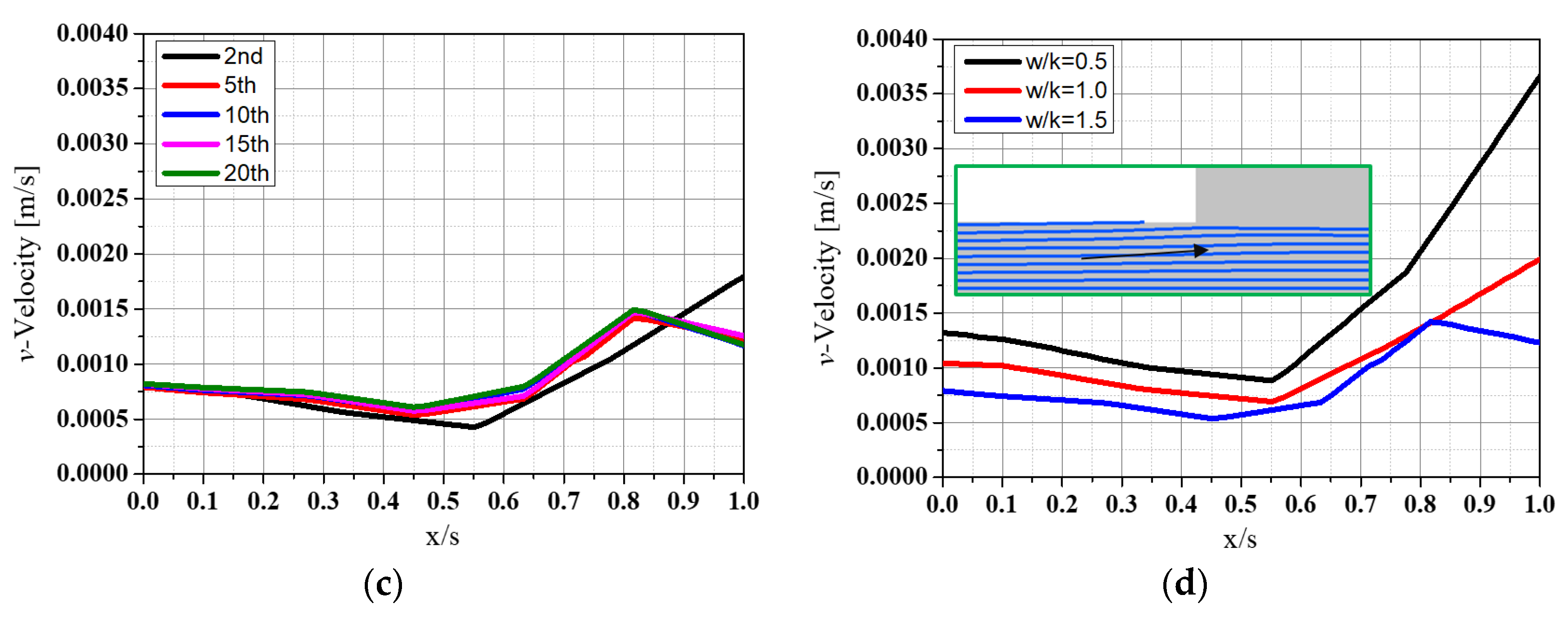
2.3. Grid Independent Test

A grid independence test was carried out to obtain accurate analysis results and to find an appropriate grid size. Figure 3 shows the grid for numerical analysis. A hexahedral mesh is used. In order to satisfy the log-law of the turbulent velocity distribution adjacent to the wall, y+ was set less than 12. For the corrugated pipe, the flow in the groove is more important than the main flow inside the pipe. Therefore, the grid independent test was performed by changing the Δy size of the grid only inside the groove and decreasing Δy from 0.28 mm to 0.20 mm. where Δy is the y-direction length of grid.
The y+ value at the first node point is fixed. However, if the mesh size suddenly increases from the node point at the wall and the next node point Δy, a numerical error may occur. Therefore, the mesh size increases gradually from the first node point and the mesh size becomes 0.20 mm, and 0.28 mm. We compare the v-velocity at interface and the friction factor, where v-velocity represents the y-direction velocity component. Figure 4 shows v-velocity distribution at interface different Δy. There is no difference in the v-velocity distribution of Δy = 0.28 mm and 0.24 mm. Table 2 is the result of the friction factor and the number of grids. The friction factor is calculated using the Darcy-Weisbach equation:
Δ p = f   l d ρ V a v g 2 2
where Δp is the pressure drop of the corrugated pipe, l is pipe length, d is the corrugated pipe inner diameter, ρ is the fluid density, and Vavg is the average velocity.
The result of the friction factor and the result of v-velocity distribution at the interface is similar. The number of grids was selected as 1,754,918 grids.

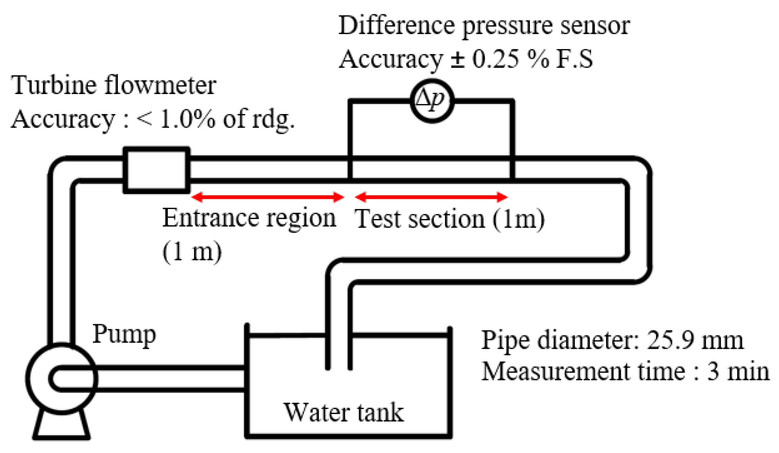
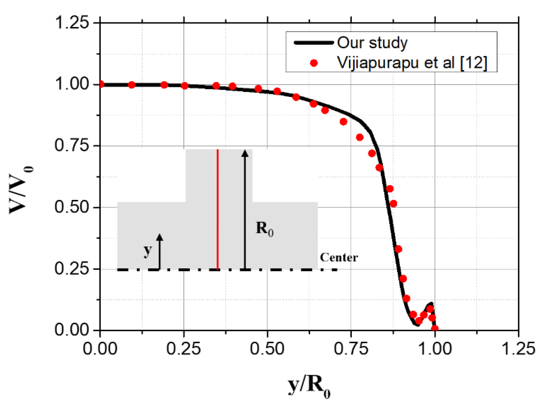
2.4. Numercial Analysis Validaiotn

The numerical analysis was validated by comparison with the experimental results. The experimental apparatus is shown in Figure 5. A turbine flowmeter was used, and a pipe length of 1 m was installed on the front of the test section, to ensure a fully developed flow before entering the test section.
The experiment was conducted using water in a Reynolds number range of 43,000 to 70,000. The pressure difference was measured at the inlet and outlet of the pipe. Since it was turbulent flow, the pressure difference was measured for 3 min due to the fluctuation of the measurement, and it was represented as the average value. Table 3 represents the results of the experiment with those of the numerical analysis. The value of friction factor by experiments and numerical analysis are represented as fexp and fnum and correlates with 95.5% to 98.9%. The results of the experimental and numerical studies demonstrated a similar tendency within an error range up to about four percent. In addition, to validate the turbulence model we used, the velocity distribution inside the corrugated pipe was compared. Figure 6 shows the comparison of the velocity profile at the center of the groove between our study and Vijiapurapu et al. [12] where, V is the velocity distribution, V0 is the velocity at the center line, and R0 is outer the corrugated pipe radius. The velocity profile differs by up to 8.5%. The numerical method has been validated.

3. Results and Discussion

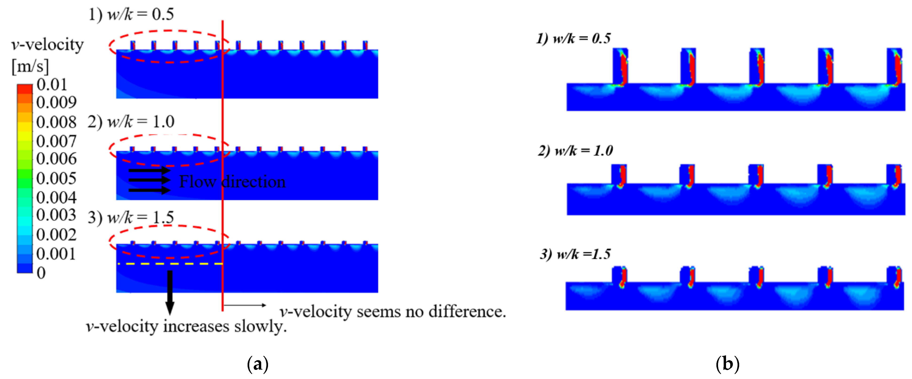
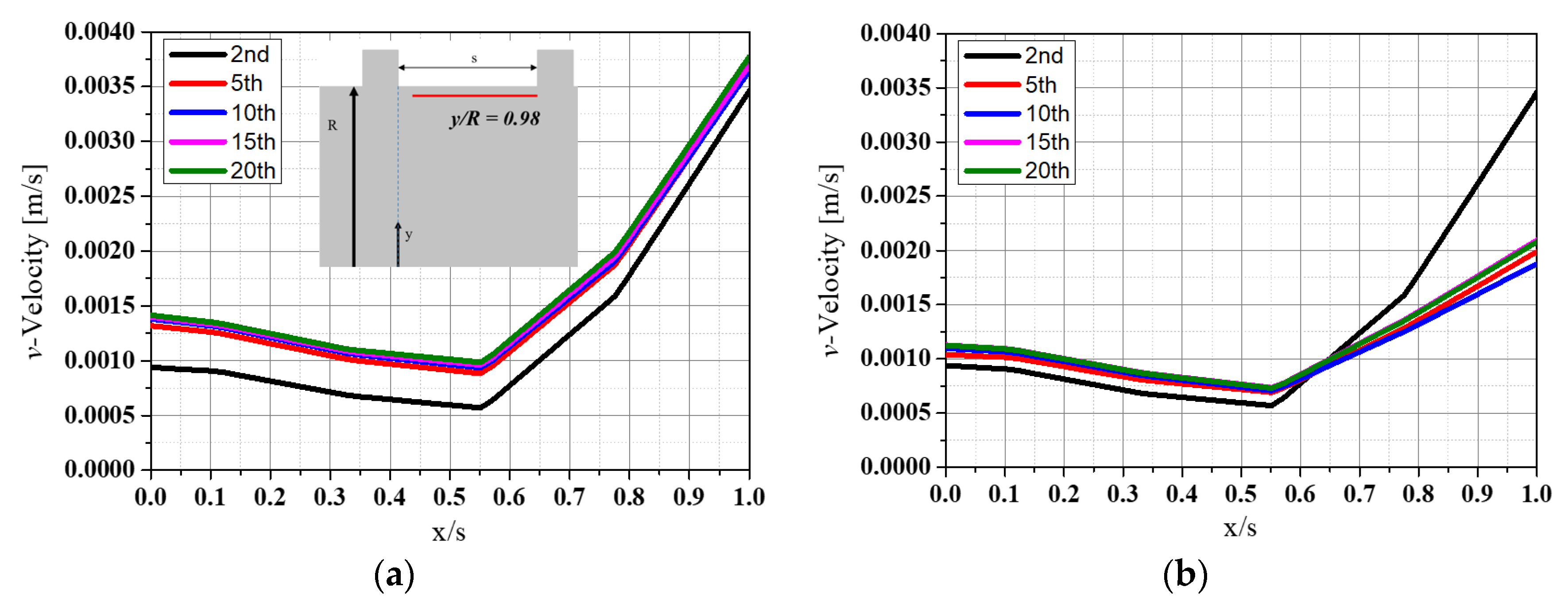
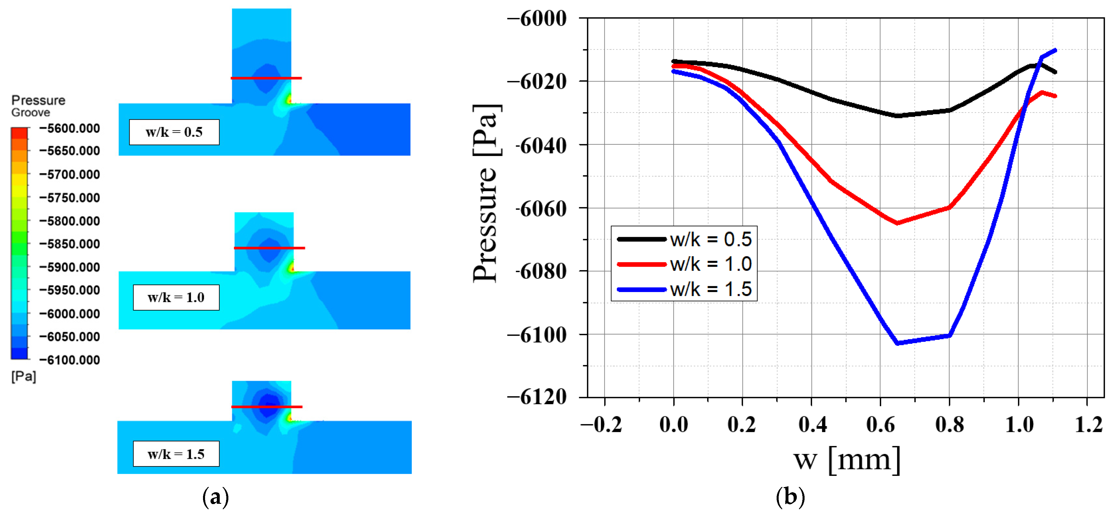
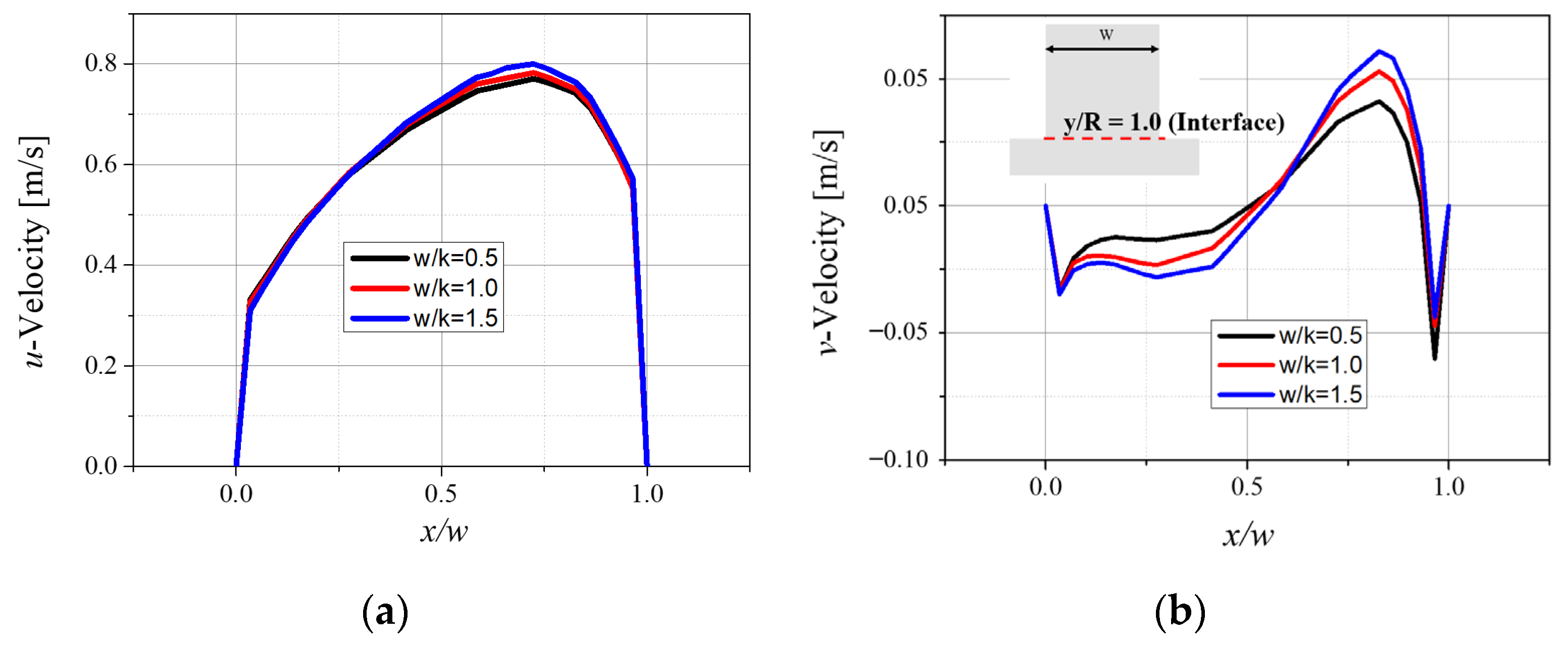
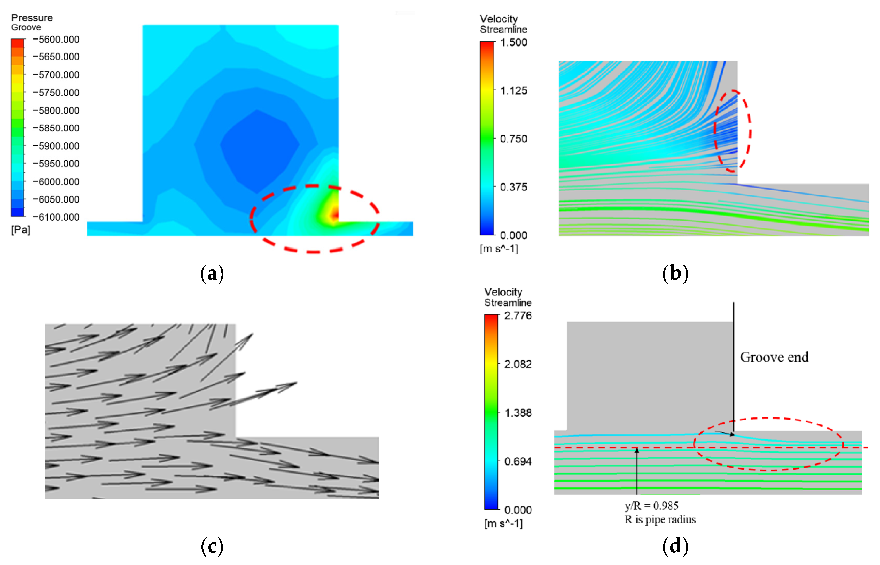
3.1. The Effect of the Groove Height

Figure 7 shows the internal flow of the corrugated pipes for three different heights, w/k = 0.5, 1.0, and 1.5, respectively. The magnitude of v-velocity near the wall between grooves is larger. This means that flow near the wall can go to the next grooves. Furthermore, the v-velocity increased gradually until the 5th groove, but remained constant after that.
Figure 8 represents the v-velocity distribution for each case at y/R = 0.98 near the pipe wall, represented as the red line. The v-velocity profiles on (a)~(c) containing the 2nd to 20th grooves were analyzed for the various ratios of w/k = 0.5, 1.0, and 1.5, respectively. The enlarged v-velocity profiles on three ratios at the 5th groove are shown in (d). The v-velocity profiles between the 2nd groove and 5th groove are different, but subsequent to the 5th grooves, are not significant. The interactions between grooves at the following 5th groove appear the almost same. Thus, the flow analysis was conducted after the 5th groove. Since the value of w is fixed, and the ratio is relative to k, the large number of w/k ratio means a small groove height. A lower height of the groove represents less flow in the v-direction, causing less transfer of velocity. As w/k increases, so does the v-velocity. Within the range of 0.5 < x/s, the v-velocity has been increasing in all cases. Furthermore, in the case of w/k = 1.5, v-velocity has been decreasing when x/s is greater than 0.8. This is reflecting that the main flow affects the groove before entering the groove, as represented in streamline in Figure 8d with a green-colored border.
Figure 9 shows the pressure contours and distribution at the red line. Due to the primary vortex center, the pressure at the center of the groove appears to be the lowest. The lower the height, the lower the pressure in the center of the groove. Because the lower the groove height, the faster the vortex rotational velocity. Also, we can see the high-pressure region at the lower right corner of the groove. This is the result of part of the main flow collisions at the lower right corner of the groove.
Figure 10 a,b illustrate the velocity vectors in grooves and v-velocity profiles at the red line, respectively. The lower the height, the larger the peak values of v-velocity. The velocity vector plot shows that the secondary vortex occurs in the upper right corner. These secondary vortexes are all different in shape according to the change in groove height. The change in the positive peak value shows more differences than the change in the negative peak value. The region of the secondary vortex is more significant as the groove height increases. Moreover, the secondary vortex rotates opposite to the primary vortex. Due to the secondary vortex, the difference between the positive peak values occurs according to the height.
Figure 11 represents the velocity profiles at the interface between the groove and the main flow. Profiles of (a) and (b) represent u-, and v-velocity profiles, respectively. For the u-velocity, it increases as the height decreases. Where u-velocity is the x-direction of the velocity component. For the v-velocity, the lower the height, the magnitude of v-velocity is larger at the groove interface because the flow rotates faster inside the groove. The maximum negative v-velocity values are shown at x/w = 0.9. For w/k = 1.0 and 1.5, the maximum negative v-velocity is almost same, but w/k = 0.5 it is different.
Figure 12 shows (a) is the pressure contour at the groove, (b) is the streamline at the lower right corner of the groove, (c) is the velocity vector at the lower right corner of the groove, and (d) is the streamline of the main flow. In the pressure contour, the high pressure at the lower right corner occurs because the part of the main flow impacts the lower right corner of the groove. After a collision, some of the flow enters the grooves again and rotates, with any remaining flow beyond the groove affecting the main flow. The same result can be confirmed in Stel. [10]. In the main flow’s streamline, it is affected by the flow coming out of the groove following collision.
Therefore, the velocity distribution of the main flow will be different due to the maximum negative v-velocity. Figure 13a–c are the main flow velocity distributions at the end of the groove for w/k = 0.5, 1.0, and 1.5, respectively, and (d) is an enlarged figure of w/k = 1.5. When comparing the velocity distribution at the end of the 5th and 6th groove, there is no difference in the velocity distribution. However, when comparing the 5th and 25th velocity distributions, the main flow velocity profile increases when y/R < 0.811 and decreases the range of 0.811 < y/R. This means that when passing through a single groove, the deformation of the main flow is small because the maximum negative v-velocity is lower after the collision. However, the flow after the collision still affects the main flow. Thus, this effect cannot be ignored if the number of grooves increases.
Table 4 represents comparing the results of calculating the friction factor using the Darcy-Weisbach equation and the numerical results of the smooth pipe. When comparing smooth pipes, the friction factor of the corrugated pipe was 2.73 times to 2.916 times. This result is due to the deformation of the velocity distribution of the main flow because of the out flow after the collision. In the cases of w/k = 1.0 and 1.5, the region of the secondary vortex is small, and the shape of the secondary vortex is similar. However, for the w/k = 0.5, the secondary vortex is different. To maintain this secondary vortex, the primary vortex rotation speed must be slow. Therefore, the flow out of the groove after collision is different. Since the primary vortex rotates faster, the flow after the collision enters the groove faster. Conversely, the flow out of the groove after the collision is slower. The friction factor is highest in the w/k = 0.5. The magnitude of maximum negative v-velocity is largest due to the flow out of the groove after the collision. The shape of the secondary vortex depends on the groove height, and as the height decreases, there is a critical height that can ignore this effect.

3.2. The Effect of the Groove Pitch

It has been determined that there is an interaction between the main flow and flow in grooves as a function of height. However, as the groove pitch decreases, the flow from the groove may enter the next groove, and interaction may occur between them. According to a study by Stel et al. [11], friction factor increases as the pitch decreases. Therefore, the groove pitch was reduced based on the height of w/k = 1.5, which has the most flow in and out of the groove interface, as summarized in cases 3, 4, and 5 in Table 1.
Figure 14 is a result of a comparison of the v-velocity profiles by the groove pitch at the 5th groove and 20th groove interfaces. The difference for each pitch is insignificant, and the v-velocity distribution at the 5th and 20th have similar trends.
The v-velocity distribution in the 5th and 20th grooves for each case was compared in order to analyze them in more detail. Figure 15 shows v-velocity distribution at the 5th groove and 20th groove at the interface. Figure 15a–c represent the v-velocity at the interface, and d–f represent the v-velocity at the end of the groove. There is no difference between the 5th and 20th v-velocity distributions. This indicates that the flow out of the groove after the collision has little effect on the flow of the next groove.
Figure 16 shows the main flow velocity distribution at the ends of the 5th and 20th grooves according to the pitch change. Similarly to the previously discussed height change, a difference in velocity between the 5th and 20th main flow occurs due to the flow out of grooves.
Table 5 shows the pressure drop and the friction factor for the different pitch. As the groove pitch decreases, the friction factor increases. The decrease in the pitch means that the number of grooves increases. As the number of grooves increases, the main flow is more affected by the flow out of groove after the collision.
For groove pitch, the v-velocity distributions at the groove end and interface are almost same between the 5th groove and the 20th groove when the groove pitch decreases. This means that the flow out of the groove does not enter the next groove. Thus, the friction factor depends on the number of grooves.

4. Conclusions

In this study, flow characteristics and their implications were numerically analyzed against changes in corrugated pipe groove height and pitch when the aspect ratio is less than four. The following conclusions were obtained:
When changing the groove height, the friction factor in the corrugated pipe is larger than a smooth pipe. It causes a deformation of the main flow due to the vortex inside the groove and the flow flowing out of the groove. We have observed that the shape of the secondary vortex depends on the groove height. As the height increases, so does the shape of the secondary vortex at the upper right corner. In cases where w/k = 1.0 and 1.5, the shape of the secondary vortex is similar, and thus the flow out of the groove is insignificant. For w/k = 0.5, the region of the secondary vortex is large, which increases the v-velocity of the out flow. Therefore, there is a critical height where there is no change in the v-velocity of the flow coming out after the collision. Moreover, for w/k = 0.5, the rotational velocity of the primary vortex is slow, and the v-velocity of the flow out of the groove after collision increases, and changes the main flow velocity profile. Therefore, the pressure drop is highest.
For groove pitch, the v-velocity distributions at the groove end and interface are almost same between the 5th groove and the 20th groove when the groove pitch decreases. This means that the flow out of the groove does not enter the next groove. Thus, friction factor depends on the number of grooves.

Author Contributions

Conceptualization, K.-B.H., D.-W.K.; investigation, K.-B.H., D.-W.K.; writing—original draft preparation, K.-B.H., D.-W.K.; writing—review and editing, J.K.; visualization, J.-S.N.; supervision, H.-S.R.; project administration, H.-S.R.; funding acquisition, H.-S.R., J.-S.N. All authors have read and agreed to the published version of the manuscript.

Funding

This research was funded by the Technology Innovation Program (‘20007978’, ‘Development of performance evaluation system of high-pressure fire pump for the fire truck using under special environment’) funded by the National Fire Agency(NFA) and This research was supported by Korea National University of Transportation in 2020.

Institutional Review Board Statement

Not applicable.

Informed Consent Statement

Not applicable.

Data Availability Statement

Not applicable.

Conflicts of Interest

The authors declare no conflict of interest.

References

  1. García, A.; Solano, J.P.; Vicente, P.G.; Viedma, A. The influence of artificial roughness shape on heat transfer enhance-ment: Corrugated tubes, dimpled tubes and wire coils. Appl. Therm. Eng. 2012, 35, 196–201. [Google Scholar] [CrossRef]
  2. Ünal, E.; Ahn, H.; Sorgüven, E. Experimental Investigation on Flows in a Corrugated Channel. J. Fluids Eng. 2016, 138, 070908. [Google Scholar] [CrossRef]
  3. Popiel, C.O.; Kozak, M.; Małecka, J.; Michalak, A. Friction Factor for Transient Flow in Transverse Corrugated Pipes. J. Fluids Eng. 2013, 135, 074501. [Google Scholar] [CrossRef]
  4. Bernhard, D.M.; Hsieh, C.K. Pressure Drop in Corrugated Pipes. J. Fluids Eng. 1996, 118, 409–410. [Google Scholar] [CrossRef]
  5. Eiamsa-Ard, S.; Promvonge, P. Numerical study on heat transfer of turbulent channel flow over periodic grooves. Int. Commun. Heat Mass Transf. 2008, 35, 844–852. [Google Scholar] [CrossRef]
  6. Perry, A.E.; Schofield, W.H.; Joubert, P.N. Rough wall turbulent boundary layers. J. Fluid Mech. 1969, 37, 383–413. [Google Scholar] [CrossRef]
  7. Tani, I. Turbulent Boundary Layer Development over Rough Surfaces. In Perspectives in Turbulence Studies; Meier, H.U., Bradshaw, P., Eds.; Springer: Berlin, Germany, 1987; pp. 223–249. [Google Scholar]
  8. Vijiapurapu, S.; Cui, J. Simulation of Turbulent Flow in a Ribbed Pipe Using Large Eddy Simulation. Numer. Heat Transfer Part A Appl. 2007, 51, 1137–1165. [Google Scholar] [CrossRef]
  9. Djenidi, L.; Antonia, R.A.; Anselmet, F. LDA measurements in a turbulent boundary layer over a d-type rough wall. Exp. Fluids 1994, 16, 323–329. [Google Scholar] [CrossRef]
  10. Stel, H.; Morales, R.E.M.; Franco, A.T.; Junqueira, S.L.M.; Erthal, R.H.; Gonçalves, M.A.L. Numerical and Experimental Analysis of Turbulent Flow in Corrugated Pipes. J. Fluids Eng. 2010, 132, 071203. [Google Scholar] [CrossRef]
  11. Stel, H.; Franco, A.T.; Junqueira, S.L.M.; Erthal, R.H.; Mendes, R.; Gonçalves, M.A.L.; Morales, R.E.M. Turbulent Flow in D-Type Corrugated Pipes: Flow Pattern and Friction Factor. J. Fluids Eng. 2012, 134, 121202. [Google Scholar] [CrossRef]
  12. Vijiapurapu, S.; Cui, J. Performance of turbulence models for flows through rough pipes. Appl. Math. Model. 2010, 34, 1458–1466. [Google Scholar] [CrossRef]
  13. Launder, B.E.; Spalding, D.B. Lectures in Mathematical Models of Turbulence; Academic Press: London, UK, 1972; p. 741. [Google Scholar]
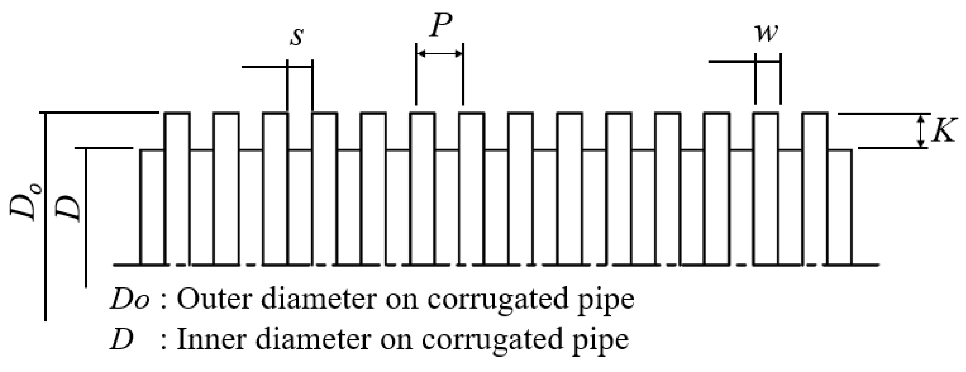
Figure 1. Explanations of the geometrics on the corrugated pipe.
Energies 14 02614 g001
Figure 2. The boundary condition for numerical analysis, and Velocity distributions for fully developed flow. (a) Computational domain and Boundary conditions, (b) Validation of fully developed flow.
Energies 14 02614 g002
Figure 3. The grids for numerical analysis (a) Pipe inlet, (b) the pipe wall, (c) in the corrugated pipe.
Energies 14 02614 g003
Figure 4. v-velocity distribution at the interface difference Δy.
Energies 14 02614 g004
Figure 5. The experimental appartus.
Energies 14 02614 g005
Figure 6. Comparing the velocity profile at the center of the groove.
Energies 14 02614 g006
Figure 7. The v-velocity contours for various ratios as a function of w/k at the corrugated pipe; (a) The v-velocity contours for the corrugated pipe different w/k, (b) The enlarged areas represented as red circle of the groove from 2nd to 5th in pipes.
Energies 14 02614 g007
Figure 8. v-velocity distribution at y/R = 0.98 for different w/k; (a) v-velocity distribution at the different groove, for w/k = 0.5, (b) v-velocity distribution at the different groove, for w/k = 1.0, (c) v-velocity distribution at the different groove, for w/k = 1.5 (d) Comparison v-velocity distribution at y/R = 0.98 for different w/k.
Energies 14 02614 g008aEnergies 14 02614 g008b
Figure 9. Pressure distribution for different w/k; (a) Pressure contour near the groove, (b) Pressure distribution at the groove center.
Energies 14 02614 g009
Figure 10. The velocity vector and distribution for corrugated pipe inside the groove: (a) The velocity vectors in the groove for the various ratios of w/k and (b) its v-velocity distribution.
Energies 14 02614 g010
Figure 11. Velocity distribution at interface for different w/k. (a) U-velocity distribution at interface line for different w/k, (b) v-velocity distribution at interface line for different w/k.
Energies 14 02614 g011
Figure 12. High-pressure region on groove corner. (a) the pressure contour at the groove, (b) the streamline at the lower right corner of the groove, (c) the velocity vector near the groove, and (d) the streamline of the main flow.
Energies 14 02614 g012
Figure 13. Main flow velocity distribution at groove end for different w/k: (a) Main flow velocity distribution at groove end for w/k = 0.5, (b) Main flow velocity distribution at groove end for w/k = 1.0, (c) Main flow velocity distribution at groove end for w/k =1.5, and (d) Velocity distribution of main flow in case of enlarged w/k = 1.5.
Energies 14 02614 g013aEnergies 14 02614 g013b
Figure 14. Comparison of v-velocity distribution at groove interface for different p/k: (a) Comparison of v-velocity distribution at 5th groove interface for different p/k, (b) Comparison of v-velocity distribution at 20th groove interface for different p/k.
Energies 14 02614 g014
Figure 15. The v-velocity distribution at the interface of the groove and main flow at the 5th and 20th case and the v-velocity at the end of the groove. (a) v-velocity distribution at interface for p/k = 7.167, (b) v-velocity distribution at interface for p/k = 4.00, (c) v-velocity distribution at interface for p/k = 3.167, (d) v-velocity distribution at groove end for p/k = 7.167, (e) v-velocity distribution at groove end for p/k = 4.00, and (f) v-velocity distribution at groove end for p/k = 3.167.
Energies 14 02614 g015
Figure 16. Main flow velocity profile at groove end for different p/k. (a) Main flow velocity profile at the groove end for p/k = 7.167, (b) Main flow velocity profile at the groove end for p/k = 4.00, (c) Main flow velocity profile at the groove end for p/k = 3.167.
Energies 14 02614 g016
Table 1. Parameters of corrugated pipe for numerical analysis.
CaseD
(mm)
s
(mm)
P
(mm)
w
(mm)
K
(mm)
w/KP/K
Case 125.94.4035.56851.16552.3310.52.389
Case 225.94.4035.56851.16551.16551.04.78
Case 325.94.4035.56851.16550.7771.57.167
Case 425.92.3313.49651.16550.7771.54.00
Case 525.91.2952.46051.16550.7771.53.167
Table 2. Grid independent test using friction factor.
Numberw/kNumber of Mesh (Δy)Friction FactorComparison
11.51,939,427 (0.20 mm)0.053426f1/f2 = 1.26%
21.51,754,918 (0.24 mm)0.052761f2/f3 = 3.48%
31.51,637,979 (0.28 mm)0.050987-
Table 3. Comparison of Experimental results and Numerical results based on friction factor.
Refexpfnumfexp/fnum
(Error Rate [%])
43,0000.02150.02240.960 (4.02)
58,0000.02010.02040.989 (1.47)
70,0000.01870.01960.955 (4.59)
Table 4. Pressure difference and friction factor as a function of w/k with comparison of the value on smooth pipe.
Casew/kFriction FactorPressure Difference [Pa]f/fsmooth
Case 10.50.05532397.2232.916
Case 21.00.05192249.8352.736
Case 31.50.05282288.8492.781
Smooth-0.0196849.6491.000
Table 5. Pressure difference and friction factor for different p/k in a single groove.
p/kFriction FactorPressure Difference [Pa]f/fp/k=7.167
7.1670.05282288.8491.000
4.000.05692466.5821.078
3.1670.06152665.9891.165
Publisher’s Note: MDPI stays neutral with regard to jurisdictional claims in published maps and institutional affiliations.

