Design of a Non-Linear Observer for SOC of Lithium-Ion Battery Based on Neural Network

Abstract

This paper presents a method for use in estimating the state of charge (SOC) of lithium-ion batteries which is based on an electrochemical impedance equivalent circuit model with a controlled source. Considering that the open-circuit voltage of a battery varies with the SOC, an equivalent circuit model with a controlled source is proposed which the voltage source and current source interact with each other. On this basis, the radial basis function (RBF) neural network is adopted to estimate the uncertainty in the battery model online, and a non-linear observer based on the radial basis function of the RBF neural network is designed to estimate the SOC of batteries. It is proved that the SOC estimation error is ultimately bounded by Lyapunov stability analysis, and the error bound can be arbitrarily small. The high accuracy and validity of the non-linear observer based on the RBF neural network in SOC estimation are verified with experimental simulation results. The SOC estimation results of the extended Kalman filter (EKF) are compared with the proposed method. It improves convergence speed and accuracy.

1. Introduction

With the shortage of resources and environmental pollution gradually becoming more serious, people are paying more attention to Battery Electric Vehicles (BEVs) due to their advantages of environmental protection, clean energy, low cost, high technology [1]. In order to ensure the safe and reliable operation of BEVs, the following items are essential components of BEVs: increasing the driving range, extending the battery life, reducing the battery cost [2,3,4], and a Battery Management System (BMS). SOC estimation is one of the main functions of a BMS [5]. Its value is directly related to battery life and safety. However, SOC cannot be measured directly, it can only be estimated by measuring variables such as current and voltage [6].

A battery model with small error and high accuracy is required, which can not only improve the accuracy of battery state estimation but also provide accurate monitoring of the important status of batteries [7]. Many methods have been proposed to estimate battery SOC, which can be divided into four main methods: open-circuit voltage methods, current time integration methods [8], data-driven methods [9,10], and model-driven methods. However, the first three methods have disadvantages such as large estimation errors, low reliability, and being time-consuming [11]. Therefore, the model-based methods have been studied by researchers because of their high interpretability and accuracy. The integer-order model is the most widely used in SOC estimation. For example, Chen et al. [12] proposed an improved Thevenin model to obtain a more accurate battery model. Considering environmental influence, Chen et al. [13] improved the battery model with the Butler–Volmer (BV) equation, which can solve the problem of large current and temperature variation.

However, compared to integer-order components, unique fractional-order components, such as CPE, can better describe the amplitude–frequency characteristics of the double layer inside the battery. For example, Liu et al. [14] proposed a fractional-order model based on the PNGV model, which considers the effects of many battery characteristics. Liu et al. [15] proposed a simplified fractional-order equivalent circuit model (FO-ECM) with high precision, which can better characterize the non-linear dynamic behaviors. However, the electrochemical process of a battery is not completely considered in this model. Electrochemical impedance spectroscopy (EIS) is widely used to establish fractional-order models, which combines both electrochemical reactions inside batteries and SOC estimation. Li et al. [16] proposed a SOC estimation method based on an equivalent circuit model in which the parameters are determined using simulated electrochemical impedance spectroscopy. Then, Hu et al. [17] established a fractional-order equivalent circuit model of lithium-ion batteries based on electrochemical impedance spectroscopy using constant-order and fractional-order characteristics such as Warburg. To improve the accuracy, Xiong et al. [18] proposed an online parameter identification method based on a fractional impedance model, which obtains the solid electrolyte interphase resistance to predict the remaining capacity. On this basis, Mawonou et al. [19] proposed a time-domain and frequency-domain fractional-order model parameter identification method based on a recursive least squares algorithm. It was proved that the fractional-order model had better performance and robustness than the classical integer-order model.

Many non-linear state estimation algorithms and adaptive filters have been studied. Typical algorithms are the Kalman filter [20,21], Luenberger observer [22], PI (proportional-integral) observer [23], H-infinity observer [24,25], sliding mode observer [26,27], particle filter [28,29,30], etc. In the SOC estimation methods based on the power battery model, the most common method is the Kalman filter, which is often used to estimate SOC based on linear battery models, but most battery models are non-linear. Therefore, many non-linear state estimation algorithms and adaptive filters are proposed to estimate or infer the internal state of batteries. To determine the non-linear characteristics of the battery mode, the improved Kalman filter has been further studied. Charkhgard et al. [31] proposed a method of SOC estimation combining a neural network (NN) and an extended Kalman filter (EKF) for SOC estimation. However, this method is based on a data-driven battery model, which has the disadvantage of poor interpretability. Focusing on this problem, Chen et al. [32] designed a SOC estimation method based on an EKF and a non-linear battery model which divides the model into a non-linear, open-circuit voltage and a second-order resistance-capacitance model. To improve the accuracy of the EKF, Zhang et al. [33] proposed a method that combines an unscented Kalman filter (UKF) and a comprehensive battery model. The system state variables are calculated recursively through a non-linear mapping process, which effectively reduces the error. However, the basic principle of the EKF algorithm is to linearize the non-linear function via first-order Taylor series expansion. This local linearization will result in large errors in the battery model when it is highly non-linear, which has limitations.

Therefore, to further improve the accuracy of SOC estimation, a non-linear SOC estimation observer was widely researched. Ouyang et al. [34] proposed an SOC non-linear observer based on the equivalent circuit model. The capacitance and resistance in the battery model were considered as a non-linear function of SOC and battery temperature, and the non-linear relationship between open-circuit voltage (OCV) and SOC was considered. However, parameter uncertainty and unknown disturbance are also key issues that affect the accuracy of SOC estimation most. In this case, a non-linear observer-based on a neural network was proposed. Chen et al. [35] designed an output feedback adaptive neural network controller combining adaptive backstepping technology with the approximation ability of the radial basis function neural network, which solves the problem of non-linear and non-strict systems. Zhao et al. [36] proposed an adaptive neural-network-based control scheme, in which a radial basis function neural network was adopted to compensate for the actuator gain fault. To further improve the accuracy of the SOC estimation, Chen et al. [37] estimated the uncertainty in the battery model online through the neural network and designed a non-linear observer based on the radial basis function neural network to estimate the SOC of the battery, which was proved to have faster convergence speed and higher precision.

The above methods only focus on integer-order models and take no consideration of the characteristics of fractional-order models. In this paper, a non-linear observer for SOC estimation with an RBF neural network, considering characteristics of lithium-ion batteries, and a fractional-order model are developed. The main contributions in this paper are (1) a fractional-order electrochemical impedance equivalent circuit model of a controlled source with the interaction of voltage source and current source is established based on electrochemical impedance spectroscopy; (2) a non-linear observer for SOC estimation with an RBF neural network is improved to estimate the uncertainty in a battery based on the fractional-order model. The remaining parts of this paper are organized as follows. Section 2 provides the fractional-order electrochemical impedance equivalent circuit model for lithium-ion batteries. Section 3 introduces the non-linear observer for SOC estimation based on a neural network. Section 4 presents the results of the simulation to verify the feasibility and superiority of the model. Finally, the conclusion is delivered in Section 5.

2. Design of Battery Model

When building a battery model, the uncertainty of the model is often large due to various reasons, and the error of the SOC estimation is large. In this paper, using the uncertainty of an RBF neural network estimated in a battery model online, the SOC of a battery could be estimated more accurately. In order to accurately estimate the SOC of a battery, an intuitive and comprehensive battery equivalent circuit model was adopted.

In the modeling process of lithium-ion batteries, the characterization parameters used are the voltage, the current and the temperature of the battery. These parameters are acquired by the method of time domain data acquisition. Compared with time domain signals such as voltage, current and temperature, the impedance-frequency relationship of lithium-ion battery in a specific frequency range constitutes EIS (Electrochemical impedance spectroscopy). EIS impedance spectroscopy is a non-invasive electrochemical analysis method. Its measurement results can not only analyze the performance degradation and aging state of batteries, but also provide data support for battery modeling and low-temperature heating strategies. It is related to multiple parameters, such as SOC estimation, internal temperature monitoring, SOH life estimation and internal failure prediction. In the EIS measurement process, the general frequency band covers 0.1Hz-10kHz, the excitation and response signals are weak and usually less than 5mV, the measurement period is long and generally within tens of seconds and minutes, the signal-to-noise ratio is below -85dB, and the time window of measurement is short be less than or equal 1 second. So EIS measurement method is too complicated, and the online measurement is difficult.

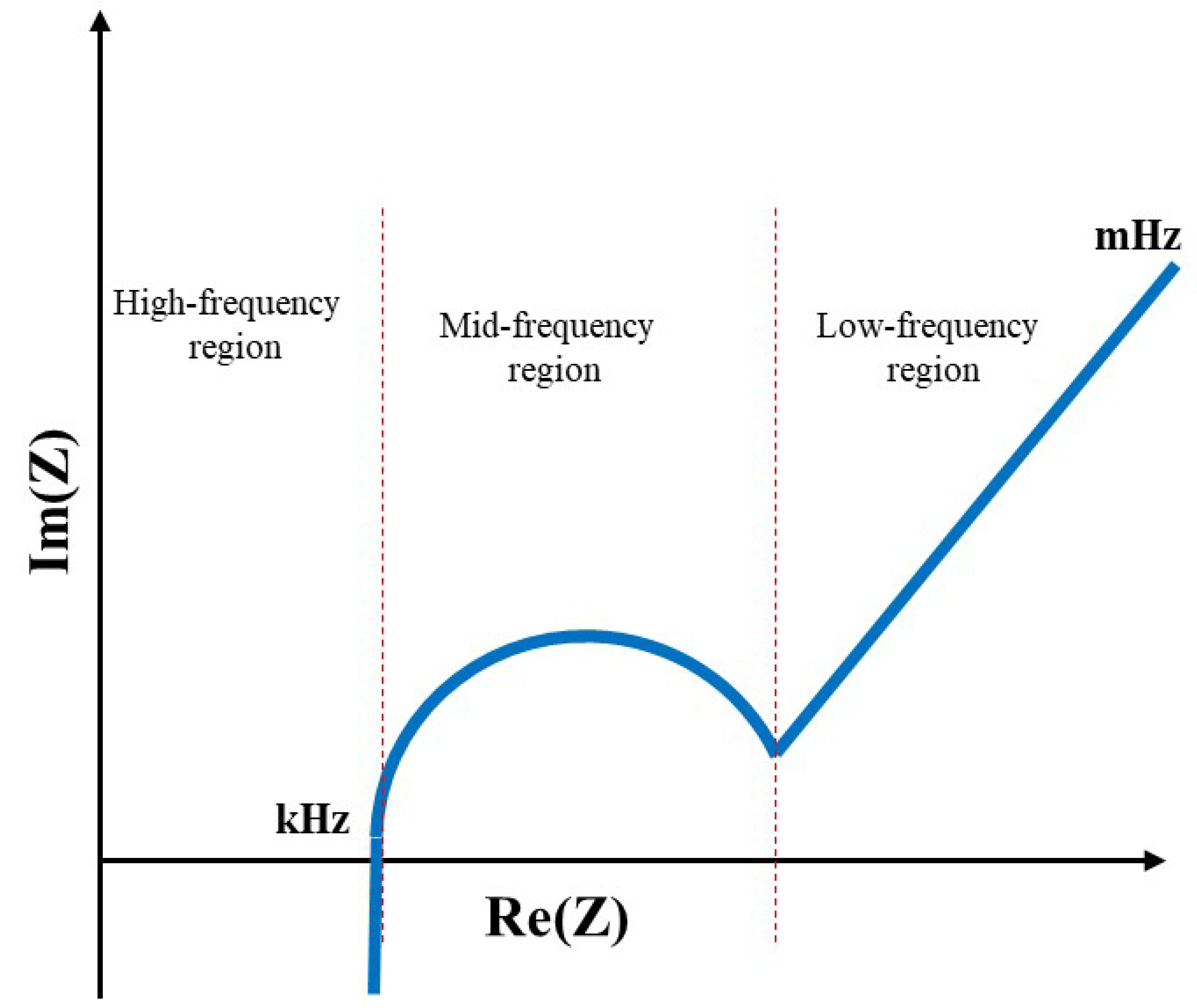
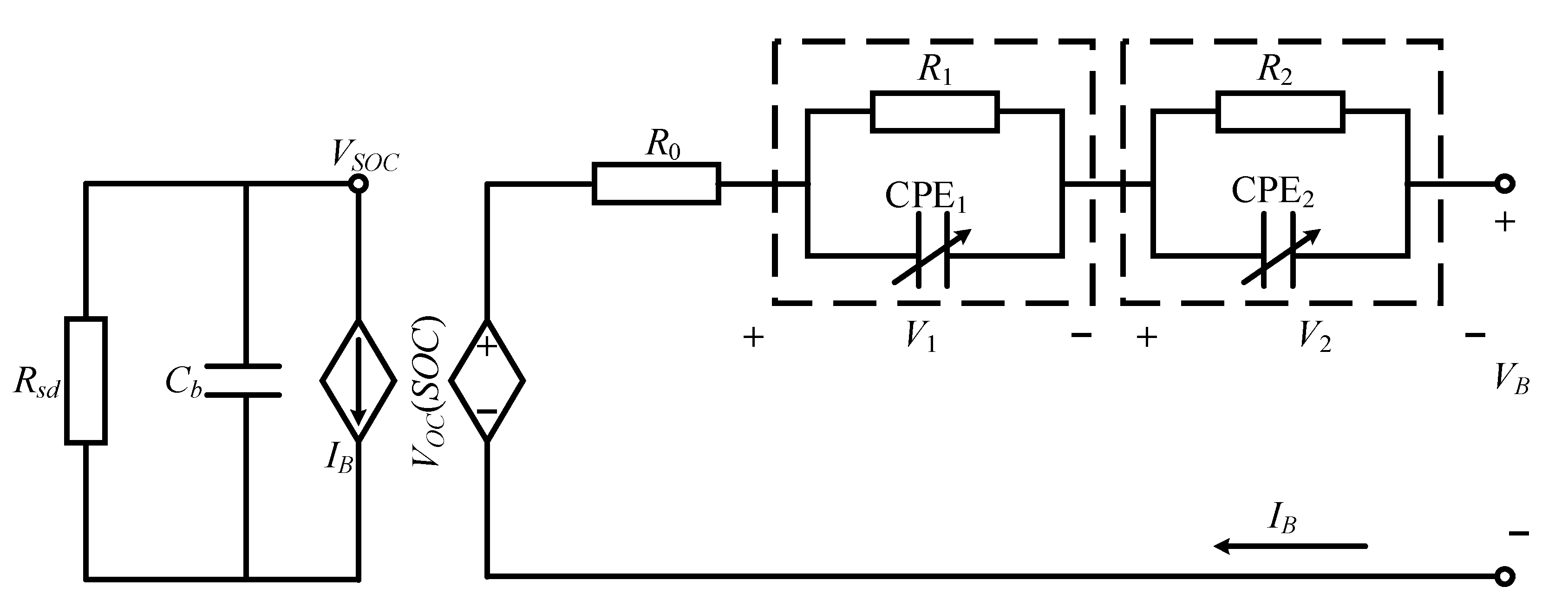
As shown in Figure 1, a typical EIS impedance spectrum is usually displayed on a negative Nyquist Diagram, with the real part of the impedance on the X-axis and the negative imaginary part of the impedance on the Y-axis. With X-axis as reference, the left side is the high frequency band. The intersection of this curve and the abscissa is the ohmic resistance of the lithium battery; the middle is the medium frequency band. The shape and parameters of this curve are formed at the interface between the lithium battery motor and the electrolyte. The electric double layer is related and is dominated by the RC parallel connected circuit, which includes the constant phase angle element (CPE); the right side is the low frequency band, and the EIS curve is a straight line with a constant slope, which is closely related to the interior of the lithium-ion active material particles. related to the solid diffusion process. It can be seen from the curve shape of EIS that lithium-ion batteries have typical fractional-order characteristics, while in the analysis process of EIS, a more accurate expression can be obtained by replacing the RC parallel component by fractional-order components. Therefore, in the ordinary second-order RC circuit model, the two capacitors are replaced by fractional-order components, and the battery model will be more accurate. The electrochemical impedance equivalent model is shown in Figure 2.

Figure 2 shows a battery electrochemical impedance equivalent circuit model with two subcircuits that interact with each other with a voltage-controlled voltage source and current-controlled current source. The left circuit in Figure 1 is used to simulate the SOC of a battery and the remaining operating time. The capacitance C_b is used to represent the total charge stored in a battery, and the R_sd is the self-discharge resistance. The capacitance C_b value is the rated capacity of the battery Q_N: C_b = Q_N. When the battery is charged, the charge amount on the capacitance C_b is set as Q and the charging current as I. In addition, $SOC={\displaystyle {\int }_0^{t}i\left(t\right)}dt/Q_N=Q/Q_N$ $=C_b\cdot V_{SOC}/Q_N=V_{SOC}$ is obtained by Q = C_b·V_SOC.

In Figure 2, V_SOC quantitatively represents the SOC of batteries, and V_SOC ∈ [0 V, 1 V] corresponds to 0–100% of the battery SOC. Voc(SOC) is the OCV of batteries. The non-linear mapping of SOC to OCV of batteries V_OC = f(V_SOC) = f(SOC) can also be fitted with polynomial function. V_B is a directly measurable battery end voltage. R₀, R₁ and R₂ are ohm resistors, and V₁ and V₂ are the terminal voltages of CPE₁ and CPE₂.

The mathematical model of the battery model shown in Figure 2 is established as follows:

$$\left\{\begin{array}{c}{D}^{r_1}{V}_1=-\frac{1}{R_1\left(SOC\right)C_1\left(SOC\right)}{V}_1+\frac{1}{C_1\left(SOC\right)}{I}_B\hfill \\ D^{r_2}{V}_2=-\frac{1}{R_2\left(SOC\right)C_2\left(SOC\right)}{V}_2+\frac{1}{C_2\left(SOC\right)}{I}_B\hfill \\ \hspace{1em}\hspace{1em}\hspace{1em}{\dot{V}}_{SOC}=-\frac{1}{R_{sd}{C}_b}{V}_{SOC}-\frac{1}{C_b}{I}_B\hfill \\ \hspace{1em}\hspace{1em}\hspace{1em}{V}_B=V_{OC}-V_1-V_2-R_0\left(SOC\right)I_B\hfill \end{array}\right.$$

(1)

where ${{\displaystyle D}}_t^r$ is used to represent the derivative or integral of arbitrary-order r with respect to t. The Grunwald–Letnikov definition is used in this paper [38].

Considering modeling errors, sensor measurement errors and unknown interference in real processes, the above Equation (1) battery model can be rewritten as follows:

$$\left\{\begin{array}{c}{D}^{r}x\left(t\right) =A\left(x\right)x\left(t\right) +B\left(x\right)u \left(t\right)\hfill \\ y\left(t\right)=Cx\left(t\right) +D\left(x\right)u\left(t\right) +f\left(x\left(t\right) \right)+\phi \left(x,I_B\right)\hfill \end{array}\right.$$

(2)

where x(t) = [V₁(t) V₂(t) SOC(t)]^T is the state vector; y(t) is the battery end voltage V_B which is the output of the system; u(t) is the battery current I_B, which is the system input; r = [r₁ r₂ 1]^T is the order vector of the system; $\phi \left(x,I_B\right)$ is the uncertain item. Matrices A, B, C and D are as follows:

$$\begin{array}{c}A\left(x_3\right)=\left[\begin{array}{ccc}-h_1(x_3)& 0& 0\\ 0& -h_2(x_3)& 0\\ 0& 0& -a\end{array}\right],B\left(x_3\right)=\left[\begin{array}{c}\begin{array}{c}{g}_1\left(x_3\right)\\ g_2\left(x_3\right)\end{array}\\ -b\end{array}\right],C=\left[\begin{array}{ccc}-1& -1& 0\end{array}\right],D\left(x_3\right)=-g_3\left(x_3\right)\hfill \\ h_1\left(x_3\right)=\frac{1}{R_1\left(x_3\right)C_1\left(x_3\right)},h_2\left(x_3\right)=\frac{1}{R_2\left(x_3\right)C_2\left(x_3\right)}\hfill \\ g_1\left(x_3\right)=\frac{1}{C_1\left(x_3\right)},g_2\left(x_3\right)=\frac{1}{C_2\left(x_3\right)},\hfill \\ a=\frac{1}{R_{sd}{C}_b}b=\frac{1}{C_b},g_3\left(x_3\right)=R_0\left(x_3\right)\hfill \\ \phi \left(x,I_B\right)={\left[\begin{array}{ccc}0& 0& \psi \left(x,I_B\right)\end{array}\right]}^T\hfill \end{array}$$

(3)

The function f (x(t)) is widely used to represent OCV-SOC relationships for many batteries, which are expressed as:

$$f\left(x\left(t\right) \right)={\displaystyle \sum _{k=0}^M{d}_{k}x\left(t\right){ }^k}$$

(4)

where $d_k\left(k=0,1,\dots M\right)$ is the factor of $f\left(x\left(t\right)\right)$. According to the relationship between OCV-SOC in batteries, f (SOC) is a monotonic increasing function, and the easy Equation (4) is Lipschitz-continuous in the range of $0\le SOC\le 1$, then $\Vert f\left(SO{C}_1\right)-f\left(SO{C}_2\right)\Vert \le \gamma \Vert SO{C}_1-SO{C}_2\Vert$, where γ is the Lipschitz constant.

The coefficient of matrix A(x) in Equation (3) is related to the charging and discharging time constant, whose magnitudes are generally determined in the battery system. Therefore, the time constants can be the average value of the charge and discharge time constants under different SOCs, which are denoted as R_1cC_1c, R_2cC_2c. In this way, Equation (2) can be rewritten as

$$\left\{\begin{array}{c}{D}^{r}x\left(t\right) =Ax\left(t\right) +B\left(x\right)u \left(t\right)\hfill \\ y\left(t\right)=Cx\left(t\right) +D\left(x\right)u\left(t\right) +f\left(x\left(t\right) \right)+\phi \left(x,I_B\right)\hfill \end{array}\right.$$

(5)

where $A=\left[\begin{array}{ccc}-\frac{1}{R_{1c}{C}_{1c}}& 0& 0\\ 0& -\frac{1}{R_{2c}{C}_{2c}}& 0\\ 0& 0& -a\end{array}\right]=\left[\begin{array}{ccc}-m& 0& 0\\ 0& -n& 0\\ 0& 0& -a\end{array}\right]$, m, n > 0.

Remark 1.

Resistance and capacitance in an equivalent circuit can be assumed to be positive and bounded. Due to the protection of BMS, the charging and discharging current of the batteries is limited, and all states of the battery system are bounded by the non-limit current of the batteries. Therefore, it can be obtained that h₁(x₃) and h₂(x₃) in Equation (3) are positive and bounded, and I_B(t), x(t) and g₁(x₃), g₂(x₃), g₃(x₃) are bounded.

3. Design of Non-Linear State Observer Based on RBF Neural Network

Based on improved fractional-order electrochemical impedance equivalent circuit model with a controlled source and electrochemical impedance spectroscopy in Section 2, a non-linear observer based on a neural network, where an RBF neural network is designed to approximate the uncertainty in the battery model online, is shown in this section.

The model is shown in Equation (6):

$$\left\{\begin{array}{c} D^r\widehat{x}\left(t\right) =A\widehat{x}\left(t\right) +B\left(\widehat{x}\right)u \left(t\right)+L\left(y-\widehat{y}\right)\hfill \\ \widehat{y}\left(t\right)=C\widehat{x}\left(t\right) +D\left(\widehat{x}\right)u\left(t\right) +f\left(\widehat{x}\left(t\right) \right)+\widehat{\phi }\left(\widehat{x},I_B\right)\hfill \end{array}\right.$$

(6)

In the above equation, $\widehat{x}\left(t\right)$ is state estimation and $\widehat{y}\left(t\right)$ is the output estimation of the actual terminal voltage. L = [l₁, l₂, l₃]^T is the observer gain vector to be designed. $\widehat{\phi }\left(\widehat{x},I_B\right)=\widehat{\psi }\left(\widehat{x},I_B\right)$ is the estimate value of $\phi \left(x,I_B\right)$ in Equation (2). An RBF neural network used to estimate modeling errors and unmeasurable disturbances, as shown in Equation (7):

$$\widehat{\psi }\left(\widehat{x},I_B\right)=W^{T}S\left(\widehat{z}\right)$$

(7)

where the input vector is $\widehat{z}={\left[{\widehat{x}}^T,I_B\right]}^T$. The weight vector is $W={[{\omega }_1,{\omega }_2,\cdots ,{\omega }_n]}^T$. The number of nodes in the neural network is N. The activation function vector is $S\left(\widehat{z}\right)={\left[s_1\left(\widehat{z}\right),\cdots ,s_n\left(\widehat{z}\right)\right]}^T$, where $s_i\left(\widehat{z}\right)\left(1\le i\le n\right)$ satisfies:

$$s_i\left(\widehat{z}\right)=\exp \left[\frac{-{\left(\widehat{z}-{\mu }_i\right)}^T\left(\widehat{z}-{\mu }_i\right)}{{\eta }_i{}^2}\right]$$

(8)

The central point vector is μ_i, and the width of the Gaussian function is η_i. The adaptive law of the weight vector is:

$$\dot{W}=\Gamma \left[S\left(\widehat{z}\right)\left(y-\widehat{y}\right)-K_{\omega }W\right]$$

(9)

The positive definite constant matrices to be designed are $\Gamma ={\Gamma }^T$ and K_ω.

Remark 2.

RBF neural networks with sufficient numbers of ganglion points can approximate any continuous function. Depending on the approximation properties of RBF neural networks, the uncertainty$\psi \left(x,I_B\right)$can be replaced by the following:

$$\psi \left(x,I_B\right)=W^{\ast }{}^{T}S\left(z\right)+\xi$$

(10)

where W* is the true constant. The input vector is$z={[x^T,I_B]}^T$. An approximate error is ξ, which is assumed to be $\left|\xi \right|\le {\xi }_N$. As $\psi \left(·\right)$is bounded, and the ideal constant weight$W^{\ast }$is also bounded$\Vert W^{*}\Vert \le W_M$, in which W_M is a normal number.

The system error dynamic equation can then be obtained and is shown in Equation (11):

$$D^r\tilde{x}\left(t\right) ={\tilde{A}}_{cl}\tilde{x}\left(t\right) -\left(\tilde{B}-L\tilde{D}\right)I_B \left(t\right)+LF\left(t\right) +L\left(\phi \left(x,I_B\right)-\widehat{\phi }\left(\widehat{x},I_B\right)\right)$$

(11)

where the error between state estimation and state actual value is

$$\begin{array}{l}\tilde{x}\left(t\right)=x\left(t\right)-\widehat{x}\left(t\right)={[{\tilde{V}}_1\left(t\right)\hspace{0.33em}\hspace{0.33em}{\tilde{V}}_2\left(t\right)S\tilde{O}C\left(t\right)]}^T; F\left(t\right)= f\left(\widehat{x}(t)\right)-f\left(x(t)\right)\\ {\tilde{A}}_{cl}=A-LC; \tilde{B}=B\left(x\right)-B\left(\widehat{x}\right); \tilde{D}=D\left(x\right)-D\left(\widehat{x}\right)\\ \psi \left(x,I_B\right)-\widehat{\psi }\left(\widehat{x},I_B\right)=W^{\ast }{}^{T}S\left(x,I_B\right)+\xi -W^{T}S\left(\widehat{x},I_B\right)=-{\tilde{W}}^{T}S\left(\widehat{x},I_B\right)+\epsilon \end{array}$$

(12)

where

$$\tilde{W}=W-W^{\ast },\epsilon =W^{\ast }{}^T\left(S\left(x,I_B\right)-S\left(\widehat{x},I_B\right)\right)+\xi$$

(13)

In Equation (13), ε is the bonded term which satisfies $\left|\epsilon \right|\le {\epsilon }_M\left({\epsilon }_M>0\right)$. Since $W^{\ast }$ is a constant weight vector, $\dot{\tilde{W}}=\dot{W}$ holds.

Before giving the main theorems, the following important lemmas are given first.

Lemma 1.

A fractional differential equation,$D^{r_i}{x}_i(t)=g_i(t),0<r_i<1$, is equivalent to the following continuous frequency distributed model.

$$\begin{array}{l}\frac{\partial z_i(\omega ,t)}{\partial t}=-\omega z_i(\omega ,t)+g_i(t)\\ x_i(t)={\displaystyle {\int }_0^{\infty }{\mu }_i(\omega )z_i(\omega ,t)d\omega }\\ {\mu }_i(\omega )=\frac{\sin (r_i\pi )}{\pi }{\omega }^{-r_i}\end{array}$$

(14)

and for$r_i=1$,$D^{r_i}{x}_i(t)=g_i(t)$ can be represented as

$$\begin{array}{l}\frac{\partial z_i(\omega ,t)}{\partial t}=-\omega z_i(\omega ,t)+g_i(t)\\ x_i(t)={\displaystyle {\int }_0^{\infty }{\mu }_i(\omega )z_i(\omega ,t)d\omega }\\ {\mu }_i(\omega )=\delta (\omega )\end{array}$$

(15)

where$g_i(t)$represents the input;$x_i(t)$denotes the output;$z_i(\omega ,t)$is the frequency distributed state variable; and${\mu }_i(\omega )$is the frequency weighting function and$\delta (\omega )$is a unit impulse function.

Theorem 1.

If the observer gains l₁, l₂, l₃ in L given in Equation (6) to satisfy inequalities (16), the estimation error of the non-linear observer shown as Equation (6) together with the adaptive law shown in Equation (9) is uniformly bounded.

$$\left\{\begin{array}{l}{l}_1<m-\frac{12p_3{l}_3^2}{p_1(a-\gamma l_3)}\\ l_2<\frac{n}{5}-\frac{4p_1{l}_1}{5p_1}\\ l_3<\frac{a}{\gamma }\end{array}\right.$$

(16)

where p₁, p₂, p₃ and γ are positive constants.

Proof. 

According to Lemma 1, Equation (11) can be exactly converted into

$$\begin{array}{c}\frac{\partial z(\omega ,t)}{\partial t}=-\omega z(\omega ,t)+A_{cl}{e}_x(t)+Lh\left(e_x(t)\right)+(E-LF)\omega (t)\hfill \\ e_x\left(t\right)={\displaystyle {\int }_0^{\infty }\mu (\omega )z(\omega ,t)d\omega }\hfill \end{array}$$

(17)

where

$$\begin{array}{cc}\hfill z(\omega ,t)=& {\left[z_1(\omega ,t) z_2(\omega ,t) z_3(\omega ,t)\right]}^T\hfill \\ \hfill e_x\left(t\right)=& {\left[\tilde{V}b(t) \tilde{V}c(t) \widetilde{SOC}(t)\right]}^T\hfill \\ \hfill \mu (\omega )=& diag\left[\begin{array}{ccc}{\mu }_1\left(\omega \right)& {\mu }_2\left(\omega \right)& {\mu }_3\left(\omega \right)\end{array}\right]\hfill \\ \hfill =& \left[\begin{array}{ccc}\frac{\sin (r_1\pi )}{\pi }{\omega }^{-r_1}& 0& 0\\ 0& \frac{\sin (r_2\pi )}{\pi }{\omega }^{-r_2}& 0\\ 0& 0& \delta \left(\omega \right)\end{array}\right]\hfill \end{array}$$

(18)

After the equivalent transformation, the fractional-order model is transformed into a continuous frequency distributed state model. In order to obtain the convergence of the designed non-linear observer based on an RBF neural network, the Lyapunov function V(t) is chosen as follows:

$$V\left(t\right)={\displaystyle {\int }_0^{\infty }{z}^T(\omega ,t)\mu (\omega )Pz(\omega ,t)d\omega }+\frac{1}{2}\tilde{W}{\Gamma }^{-1}\tilde{W}$$

(19)

Then, Inequation (20) can be obtained.

$$\begin{array}{cc}\dot{V}(t)\hfill & ={\displaystyle {\int }_0^{\infty }\left[\frac{\partial z^T(\omega ,t)}{\partial t}\mu (\omega )Pz(\omega ,t)+z^T(\omega ,t)\mu (\omega )P\frac{\partial z(\omega ,t)}{\partial t}\right]}d\omega +\tilde{W}{\Gamma }^{-1}\dot{\tilde{W}}\\ & ={\displaystyle {\int }_0^{\infty }[-\omega z(\omega ,t)+{\tilde{A}}_{cl}\tilde{x}(t)+(\tilde{B}-L\tilde{D})I_B(t)+LF(t)}\hfill \\ & +L(\phi (x,I_B)-\widehat{\phi }(\widehat{x},I_B)){]}^T\mu (\omega )Pz(\omega ,t)d\omega \hfill \\ & +{\displaystyle {\int }_0^{\infty }{z}^T(\omega ,t)\mu (\omega )P[-\omega z(\omega ,t)+{\tilde{A}}_{cl}\tilde{x}(t)+(\tilde{B}-L\tilde{D})I_B(t)}\hfill \\ & +LF(t)+L(\phi (x,I_B)-\widehat{\phi }(\widehat{x},I_B))]d\omega -\tilde{W}{K}_{\omega }W\hfill \\ & \le {\displaystyle {\int }_0^{\infty }[{\tilde{x}}^T(t){\tilde{A}}_{cl}^T\mu (\omega )Pz(\omega ,t)+(\tilde{B}-L\tilde{D})I_B(t)\mu (\omega )Pz(\omega ,t)}\hfill \\ & +F^T(t)L^T\mu (\omega )Pz(\omega ,t)+{(\phi (x,I_B)-\widehat{\phi }(\widehat{x},I_B))}^T{L}^T\mu (\omega )Pz(\omega ,t)]d\omega \hfill \\ & +{\displaystyle {\int }_0^{\infty }[z^T(\omega ,t)\mu (\omega )P{\tilde{A}}_{cl}\tilde{x}(t)+z^T(\omega ,t)\mu (\omega )P}L(\phi (x,I_B)-\widehat{\phi }(\widehat{x},I_B))\hfill \\ & +z^T(\omega ,t)\mu (\omega )P(\tilde{B}-L\tilde{D})I_B(t)+z^T(\omega ,t)\mu (\omega )PLF(t)]d\omega -\tilde{W}{K}_{\omega }W\hfill \\ & ={\tilde{x}}^T(t)({\tilde{A}}_{cl}^{T}P+P{\tilde{A}}_{cl})\tilde{x}(t)+2{\tilde{x}}^T(t)P(\tilde{B}-L\tilde{D})I_B(t)+2{\tilde{x}}^T(t)PLF(t)\hfill \\ & +2{\tilde{x}}^T(t)PL(\phi (x,I_B)-\widehat{\phi }(\widehat{x},I_B))-\tilde{W}{K}_{\omega }W\hfill \end{array}$$

(20)

Assume $P=\mathrm{diag}\left\{\begin{array}{ccc}1/2p_1& 1/2p_2& 1/2p_3\end{array}\right\}$ and $p_1,p_2,p_3>0$ then:

$$\begin{array}{c}\dot{V}(t)\le -p_1(m-l_1){\tilde{x}}_1^2+|(p_1{l}_1+p_2{l}_2){\tilde{x}}_1{\tilde{x}}_2|+\left|p_3{l}_3{\tilde{x}}_1{\tilde{x}}_3\right|-p_2(n-l_2){\tilde{x}}_2^2\hfill \\ +\left|p_3{l}_3{\tilde{x}}_2{\tilde{x}}_3\right|-p_3(a-\gamma l_3){\tilde{x}}_3^2+|p_1[(g_1(x_3)-g_1({\widehat{x}}_3))+l_1(g_3({\widehat{x}}_3)-g_3(x_3))]I_B{\tilde{x}}_1|\hfill \\ +|p_2[(g_2(x_3)-g_2({\widehat{x}}_3))+l_2(g_3({\widehat{x}}_3)-g_3(x_3))]I_B{\tilde{x}}_2|\hfill \\ +|p_3[l_3(g_3({\widehat{x}}_3)-g_3(x_3))]I_B{\tilde{x}}_3|+\left|p_3{l}_3{\epsilon }_M{\tilde{x}}_3\right|-\tilde{W}{K}_{\omega }W\hfill \end{array}$$

(21)

Because $g_i\left(·\right)\left(1\le i\le 3\right),x_i\left(·\right)\left(1\le i\le 3\right),I_B\left(t\right)$ are bounded, Inequation (22) can be obtained.

$$\begin{array}{r}|p_1[(g_1(x_3)-g_1({\widehat{x}}_3))+l_1(g_3({\widehat{x}}_3)-g_3(x_3))]I_B|\le M_1\\ |p_2[(g_2(x_3)-g_2({\widehat{x}}_3))+l_2(g_3({\widehat{x}}_3)-g_3(x_3))]I_B|\le M_2\\ |p_3[l_3(g_3({\widehat{x}}_3)-g_3(x_3))]I_B|\le M_3\end{array}$$

(22)

Assume $\left(l_1{p}_1+l_2{p}_2\right)=N$; Inequation (23) can be obtained.

$$\begin{array}{l}\dot{V}(t)\le -p_1(m-l_1){\tilde{x}}_1^2+\left|N{\tilde{x}}_1{\tilde{x}}_2\right|+\left|p_3{l}_3{\tilde{x}}_1{\tilde{x}}_3\right|-p_2(n-l_2){\tilde{x}}_2^2+\left|p_3{l}_3{\tilde{x}}_2{\tilde{x}}_3\right|\\ -p_3(a-\gamma l_3){\tilde{x}}_3^2+p_1{M}_1\left|{\tilde{x}}_1\right|+p_2{M}_2\left|{\tilde{x}}_2\right|+p_3{M}_3\left|{\tilde{x}}_3\right|+\left|p_3{l}_3{\epsilon }_M{\tilde{x}}_3\right|-\tilde{W}{K}_{\omega }W\end{array}$$

(23)

Then, the inequation can be obtained as shown in Inequations (24) and (25).

$$\begin{array}{c}(1)-p_1(m-l_1){\tilde{x}}_1^2+p_1{M}_1\left|{\tilde{x}}_1\right|+\left|N{\tilde{x}}_1{\tilde{x}}_2\right|\le -\frac{p_1(m-l_1)}{3}{\tilde{x}}_1^2+\frac{3p_1{M}_1^2}{(m-l_1)}+\frac{3N^2}{p_1(M_1-l_1)}{\tilde{x}}_2^2\hfill \\ (2)-p_2(n-l_1){\tilde{x}}_2^2+\left|p_2{M}_2{\tilde{x}}_2\right|\le -\frac{p_2(n-l_2)}{2}{\tilde{x}}_2^2+\frac{2p_2{M}_2^2}{(n-l_2)}\hfill \\ (3)-p_3(a-\gamma l_3){\tilde{x}}_3^2+\left|p_3{l}_3{\tilde{x}}_2{\tilde{x}}_3\right|+\left|p_3{l}_3{\tilde{x}}_1{\tilde{x}}_3\right|+\left|p_3{M}_3{\tilde{x}}_2\right|+p_3{l}_3{\epsilon }_M\left|{\tilde{x}}_3\right|\le -\frac{p_3(a-\gamma l_3)}{4}{\tilde{x}}_3^2\hfill \\ +\frac{4p_3{l}_3^2{\tilde{x}}_1^2}{(a-\gamma l_3)}+\frac{4p_3{l}_3^2{\tilde{x}}_2^2}{(a-\gamma l_3)}+\frac{4p_3{(M_3+l_3{\epsilon }_M)}^2}{(a-\gamma l_3)}\hfill \end{array}$$

(24)

$$-\tilde{W}{K}_{\omega }W=-\tilde{W}{K}_{\omega }\left(\tilde{W}+W^{\ast }\right)\le -\frac{‖K_{\omega }‖{‖\tilde{W}‖}^2}{2}+\frac{‖K_{\omega }‖{‖W_M‖}^2}{2}$$

(25)

According to Inequations (24) and (25), Inequation (23) can be rewritten as Inequation (26).

$$\dot{V}\left(t\right)\le {\alpha }_1{\tilde{x}}_1{}^2+{\alpha }_2{\tilde{x}}_2{}^2+{\alpha }_3{\tilde{x}}_3{}^2-\frac{‖K_{\omega }‖{‖\tilde{W}‖}^2}{2}+M$$

(26)

where

$$\begin{array}{l}{a}_1=\frac{-p_1(m-l_1)}{3}+\frac{4p_3{l}_3^2}{(a-\gamma l_3)}\\ a_2=-\frac{p_2(n-l_2)}{2}+\frac{4p_3{l}_3^2}{(a-\gamma l_3)}+\frac{3N^2}{p_1(m-l_1)}\\ a_3=\frac{-p_3(a-\gamma l_3)}{4}\\ M=\frac{3p_1^2{M}_1^2}{(m-l_1)}+\frac{2p_2{M}_2^2}{(n-l_2)}+\frac{4p_3{(M_3+l_3{\epsilon }_M)}^2}{(a-\gamma l_3)}+\frac{‖K_{\omega }‖{‖W_M‖}^2}{2}\end{array}$$

(27)

According to the previous analysis, if Equation (14) is satisfied by l₁, l₂, l₃, and α₁, α₂, α₃ can be guaranteed to be negative. Since the initial value of Lyapunov function V(0) is bounded, the solution of the estimation error system is also uniformly bounded according to the boundedness analysis. The bounds of SOC estimation error are satisfied with $\left\{x_3\left(t\right)\le \sqrt{M/\lambda }\right\}$, in which $\lambda$ is a constant satisfied with $0<\lambda <p_3\left(a-\gamma l_3\right)/4$. If p₃ is selected as large, $\lambda$ can be selected large enough, and then the bounds of SOC estimation error can be arbitrarily small. Therefore, a non-linear observer based on an RBF neural network can accurately estimate the SOC of batteries. □

4. Experiment and Simulation Analysis

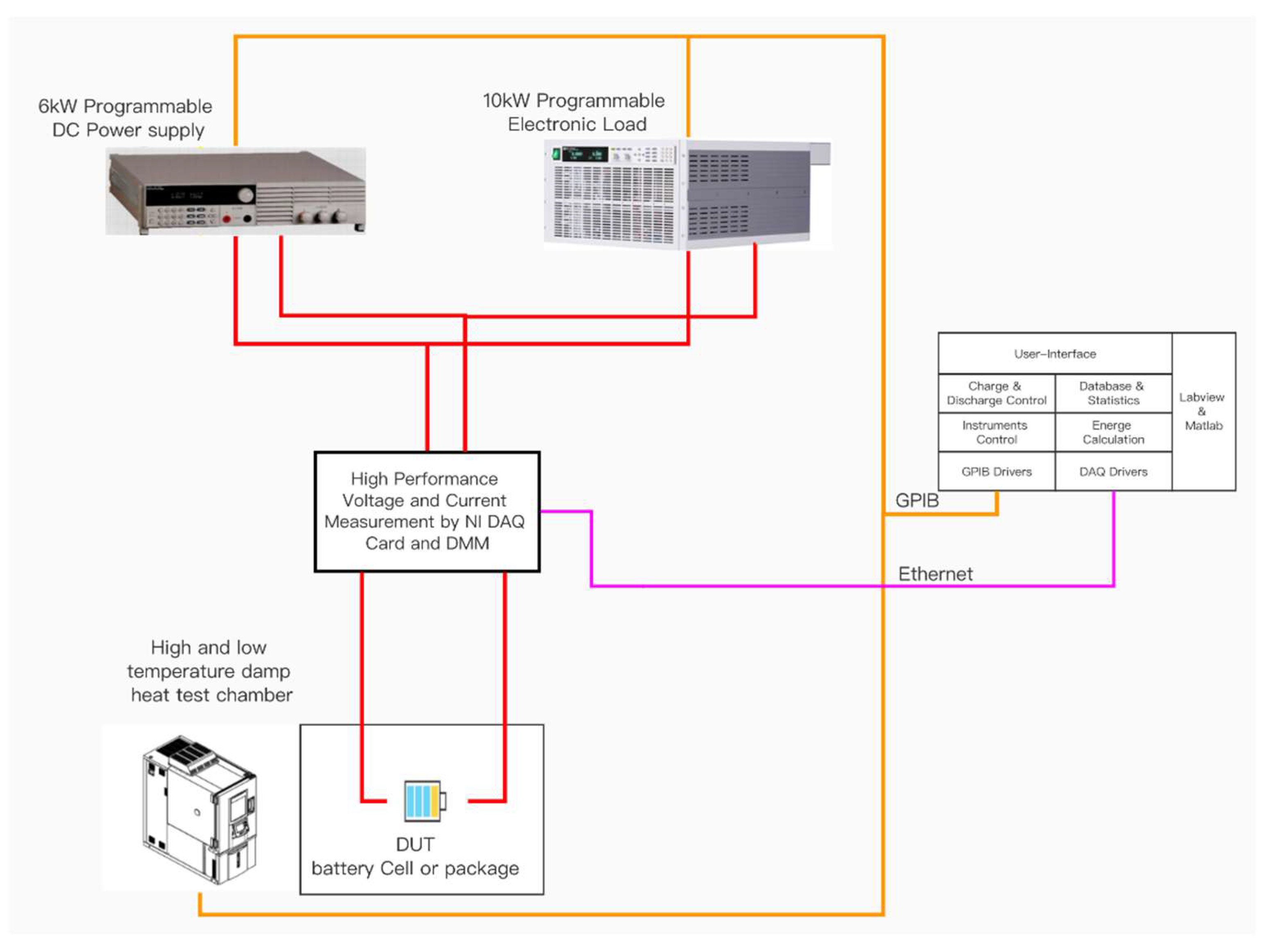
The test system was built with a PXI system developed by the National Instruments (NI). The electrical schematic diagram of the test system is shown in Figure 3, and the battery test bench was built as shown in Figure 4. The hardware platform of the battery test system was composed of four parts: an industrial computer, charging and discharging instruments, a parameter measurement device and a thermostatic humidity test box, and the software of the battery test system was designed through the LabVIEW development environment. The environmental temperature was simulated by adjusting the internal temperature of the given thermostatic humidity box. The charging and discharging instruments were controlled by a program, the charging and discharging currents of the battery were set during the experiment, and the performance test of the power battery in different environments was completed. In the process of the experiment, the current voltage and temperature of the battery were collected in real time using a high-precision voltage current and temperature sensor, and the real-time data collected were saved and exported to the table using the SQL database linked to the experimental platform.

The equipment and software list in Figure 3 is shown in

Table 1. The equipment and software list.

No.	Name of Equipment or Software	Model or Version	Functions and Performance
1	DC Power supply	IT6533A	160 V, 120 A, 6 kW
2	Electronic Load	IT8830	120 V, 500 A, 10 kW
3	USB-DAQ card	NI USB-6216	16 bit, 400 kS/s, Isolated Multifunciton DAQ
4	USB-DMM	NI USB-4065	61/2-Digit, ±300 V, 0.025%
5	Heat Test Chamber	WTH-150-40-880	−45 °C~105 °C, 99 Rh%
6	Labview	2019 SP1
7	Matlab	2019b
8	GPIB Card	NI USB-GPIB
9	USB-CAN Card	Peak CAN-USB
10	High Performance Voltage Isolated Interface	HVIS-400	Isolated Voltage: 500 V, 0.01%
11	High Performance Current Isolated Interface	HIIS-100	Isolated Voltage: 500 V, 0.01%
12	PXI Controller	NI PXIe-8840	Intel Core i7, 8 GB/s
13	PXI Chassis	NI PXIe-1062	8 slots, PXI Express Chassis

.

The test system, composed of a heat test chamber, DC power supply, electronic load and PXI system, is shown in Figure 4.

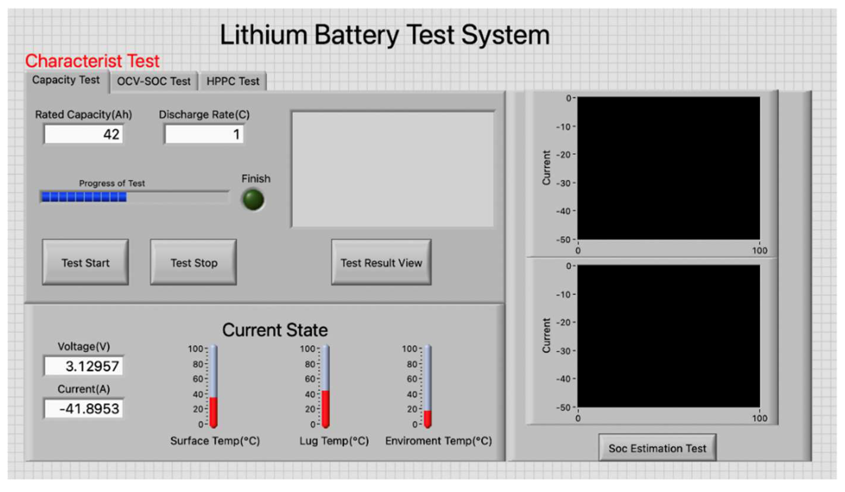
The UI of the lithium battery test system based on Labview is shown in Figure 5. The characteristic test for lithium-ion power battery could be selected on the main interface in real time, and the current size of the charger and discharger could be set. The temperature, charging and discharging current, voltage and other parameters of the battery could be displayed on the interface in real time.

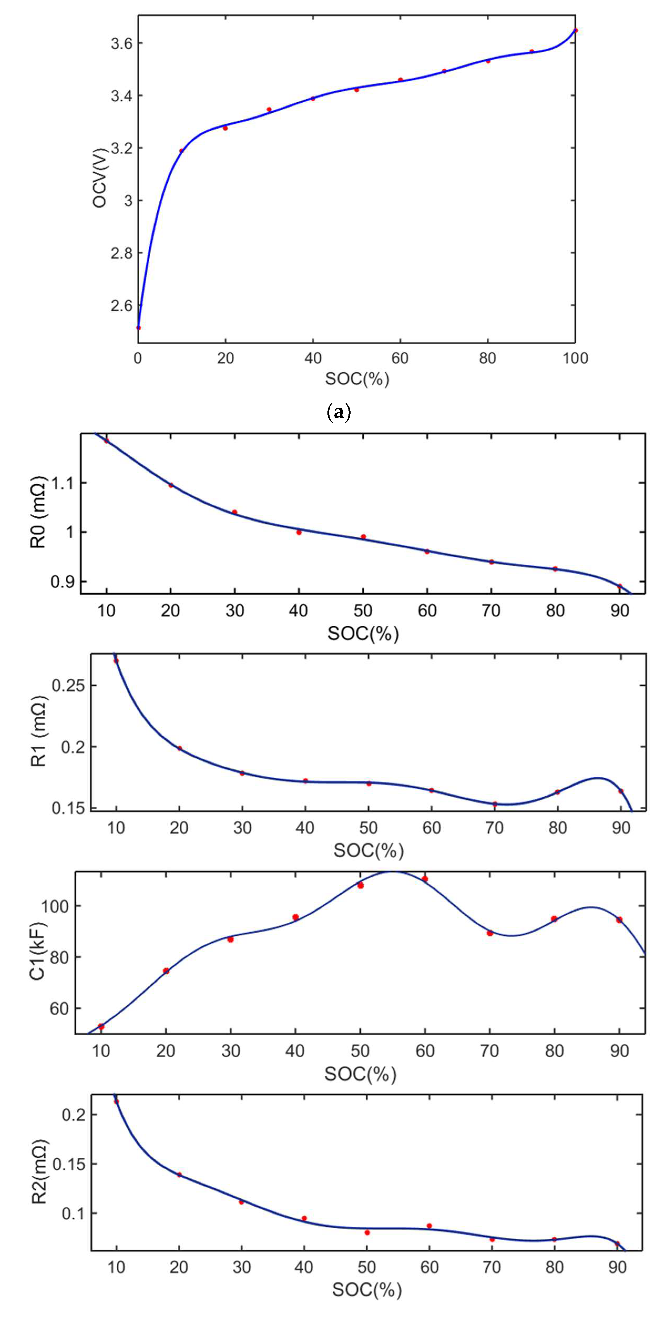
The open-circuit voltage test and HPPC test of batteries were carried out using the test and verify system. The parameters of the above model could be obtained by the least squares method. Then, these curves were fitted to balance the accuracy and complexity using an empirical equation composed of exponential and polynomial function. Figure 6a,b show the non-linear relationship between OCV and SOC of batteries and the curves between parameters (R₀, R₁, C₁, R₂ and C₂) and SOC in the equivalent circuit of batteries. The red dot is the data recorded in the test, and the blue line is the corresponding fitting curve for the actual data obtained from the experiment. The weight vector rule of the neural network is $K_{\omega }=diag(0.01,0.01,0.01,0.01,0.01,0.01,0.01,0.01)$ and $\Gamma =diag(1,1,1,1,11,1,1,1,1)$.

Figure 6a shows the curves of OCV and SOC obtained using the standard OCV test method. Figure 6b shows the measured values and fitting curves of the equivalent circuit parameters of the battery.

The battery test platform mentioned above was used to carry out three different dynamic operating conditions experiments to verify the accuracy and effectiveness of the proposed RBF neural network, non-linear, fractional-order observer. Since high-precision measuring instruments were used when building the battery test platform, the current data collected by the device had high precision. The accurate SOC could be obtained as the real reference value of SOC using the current-time integral method.

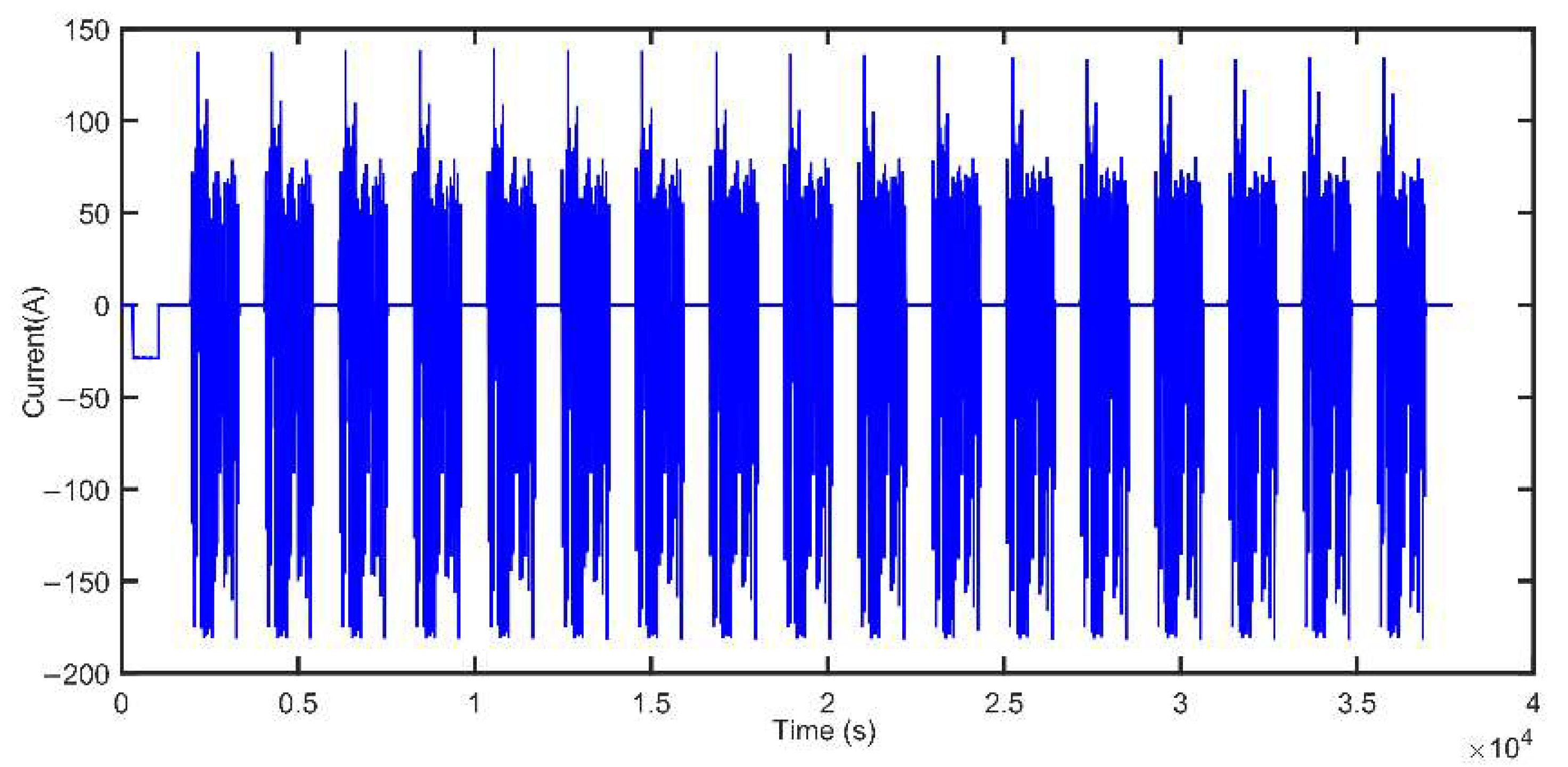
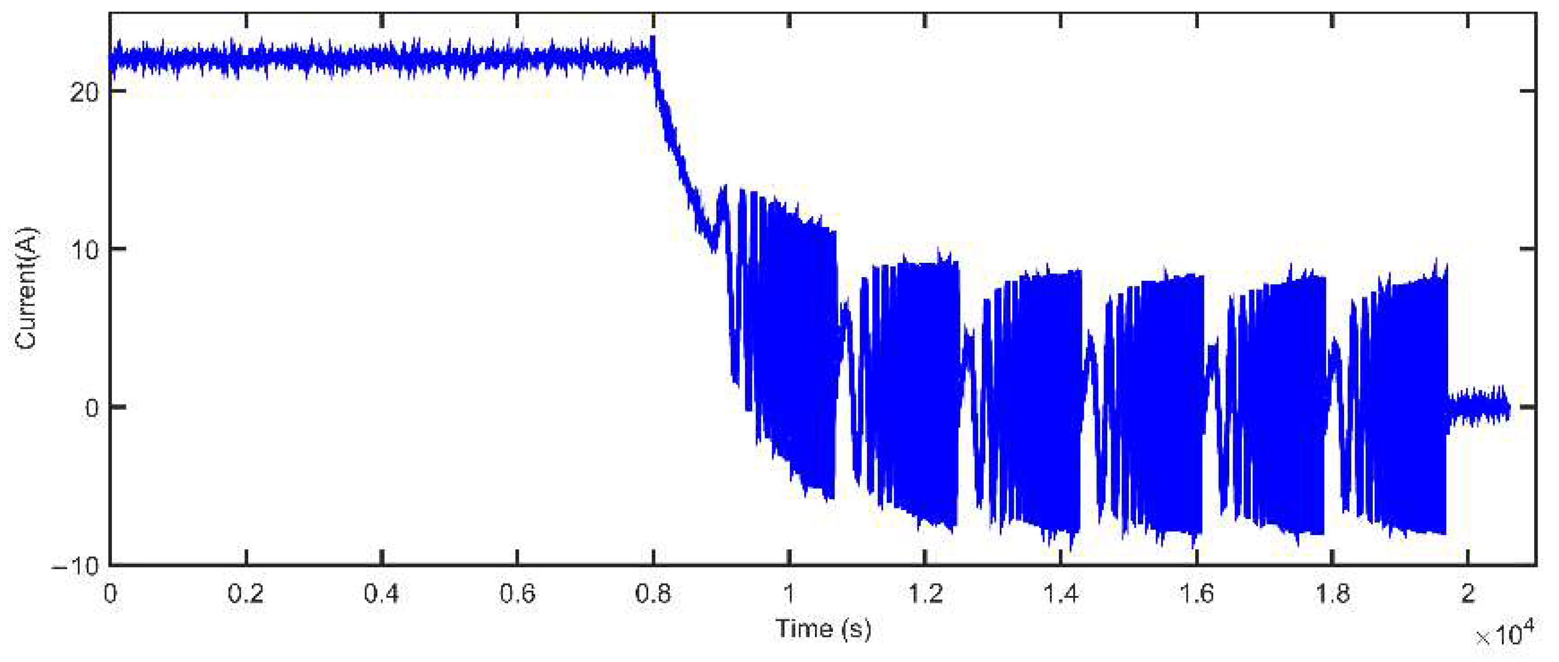
Dynamic operation test 1: Leave the fully charged battery in the incubator for 24 h at the laboratory temperature to ensure that the temperature of the entire battery is even. Use a constant current of 1C to discharge the battery at a capacity of 10% (to avoid overvoltage conditions during the subsequent dynamic operating experiment). Dynamic operation test 1 is performed within the range of SOC of interest (90% to 10% SOC). The experimental current image of Dynamic operation test 1 is shown in Figure 7.

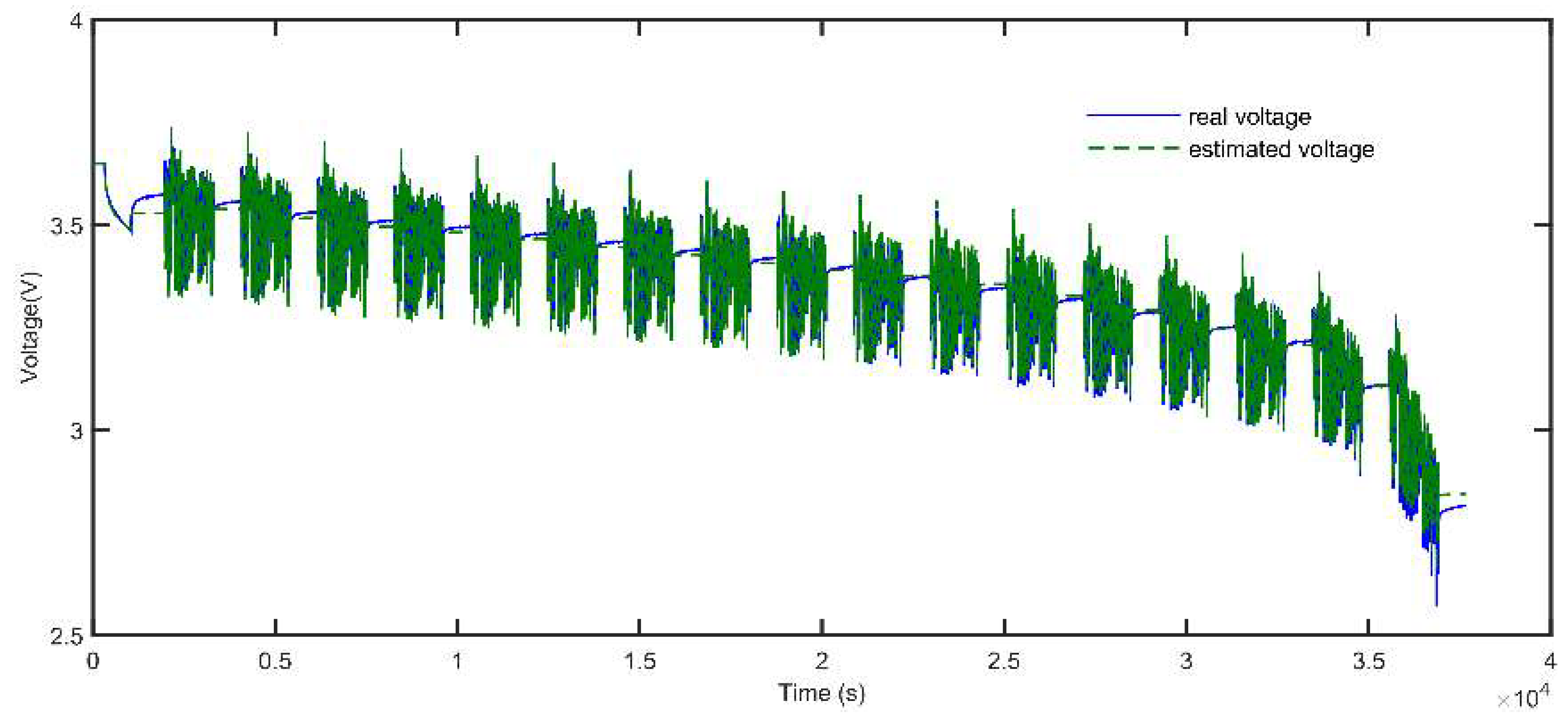
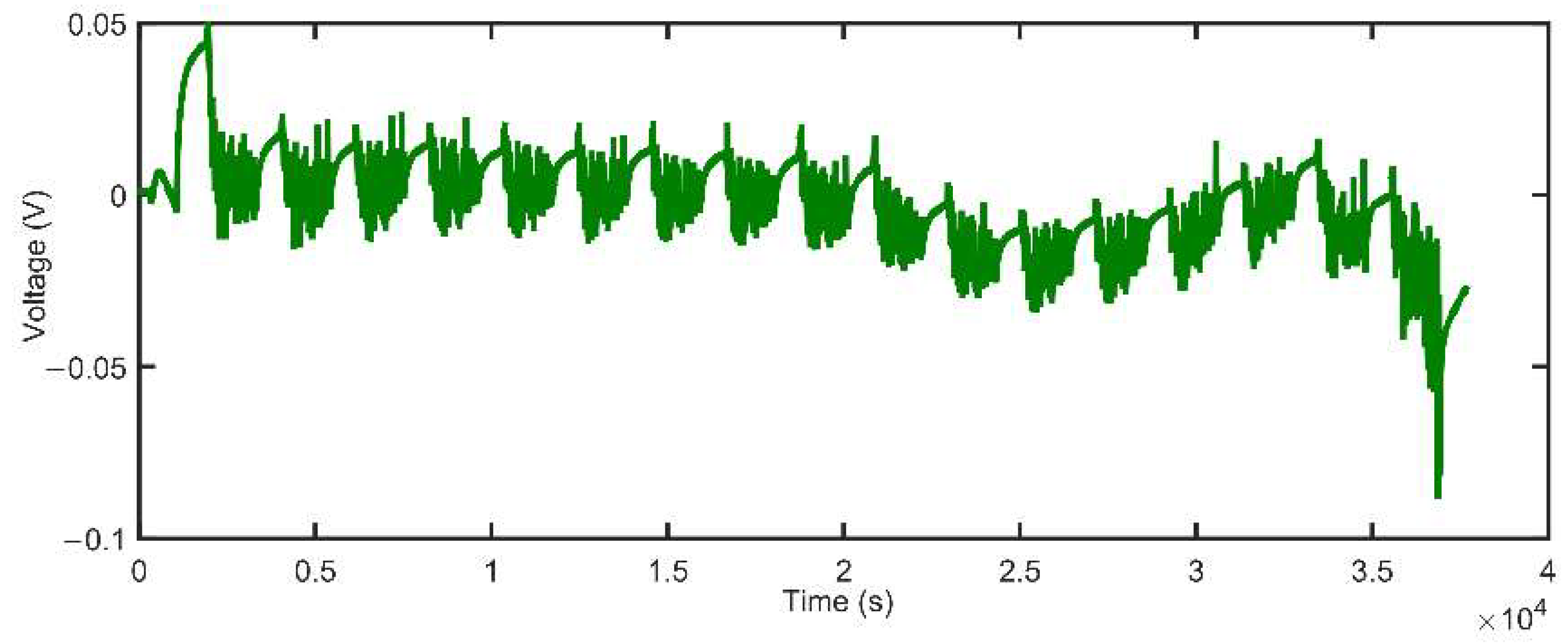
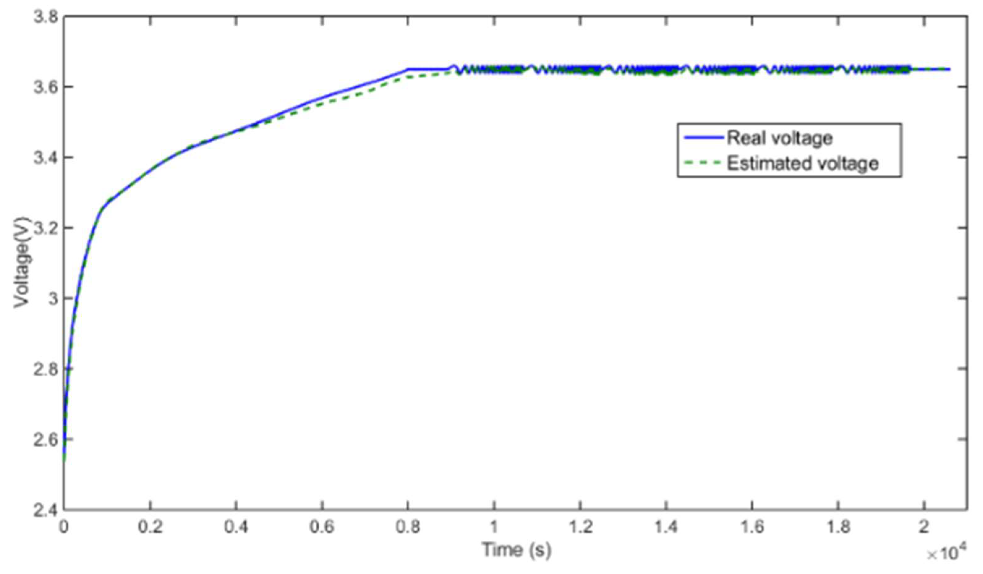
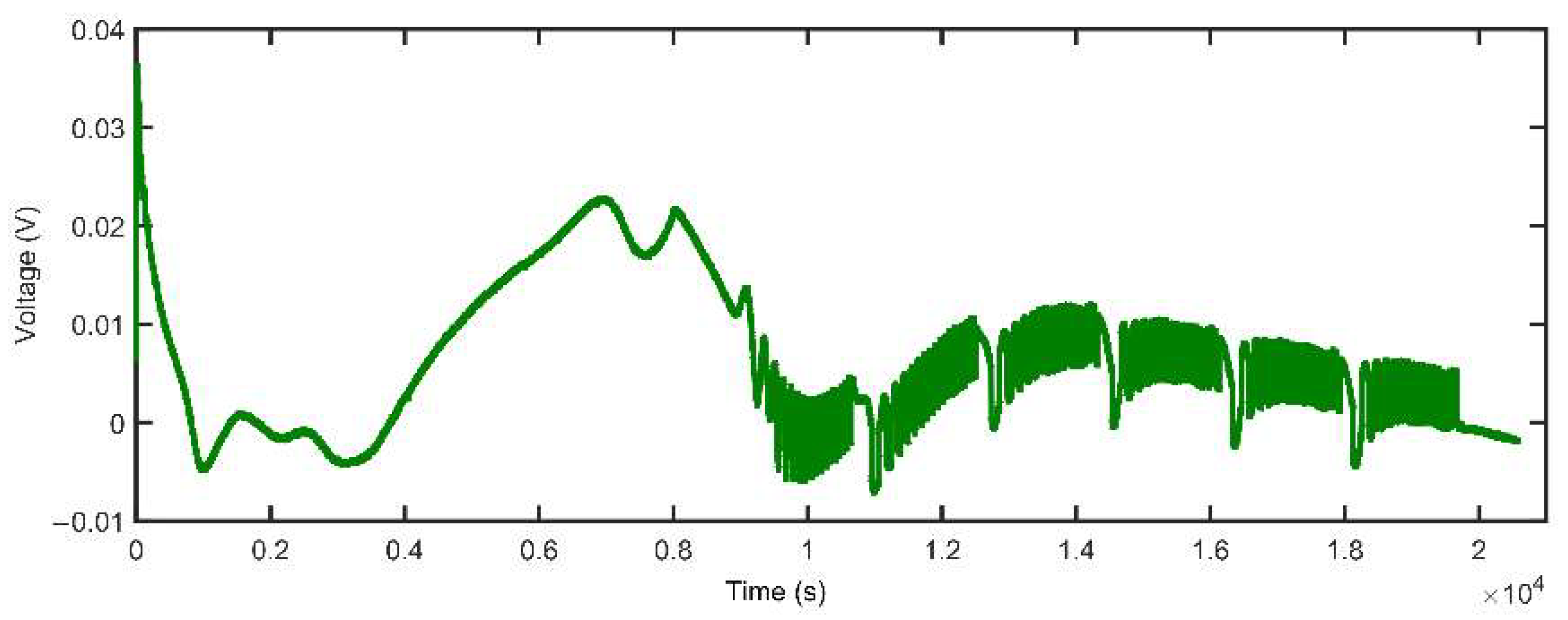
The measured actual end voltage for reference and the model estimated end voltage curves and their local amplification diagrams are shown in Figure 8 and Figure 9, respectively. The local amplification diagrams shown in Figure 9 show that the measured actual end voltage curves for reference and the curves estimated by the model basically coincide. The RMSE of the real and model results was 5.97 mV under dynamic condition test 1. The local amplification curve shown in Figure 9 shows more clearly that the identified model reflects the dynamic characteristics of the battery with high accuracy, and the proposed circuit model captures the battery performance well. The accuracy of battery SOC estimation depends on whether the battery voltage estimated by the model is accurate, which proves that the proposed model can more effectively and accurately estimate the battery status, and the corresponding voltage error curve is shown in Figure 10.

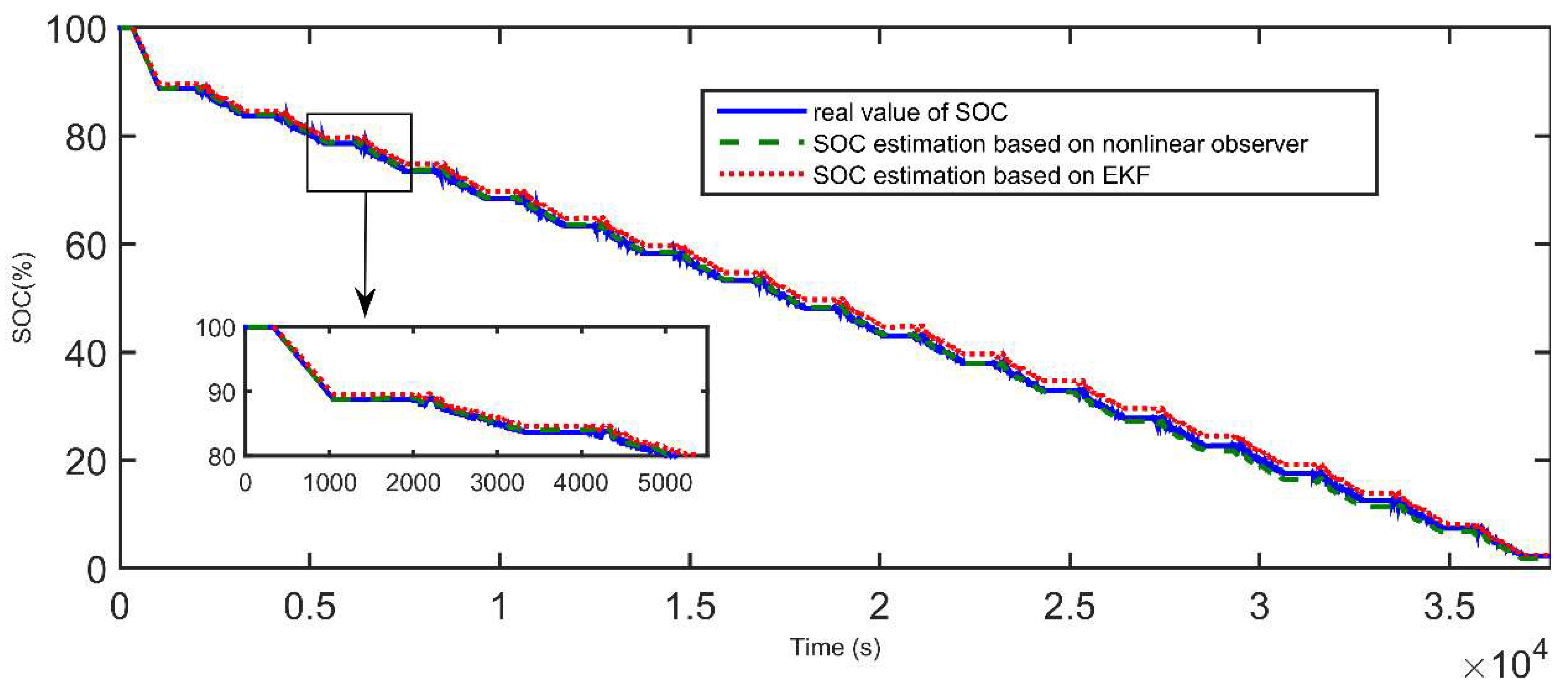
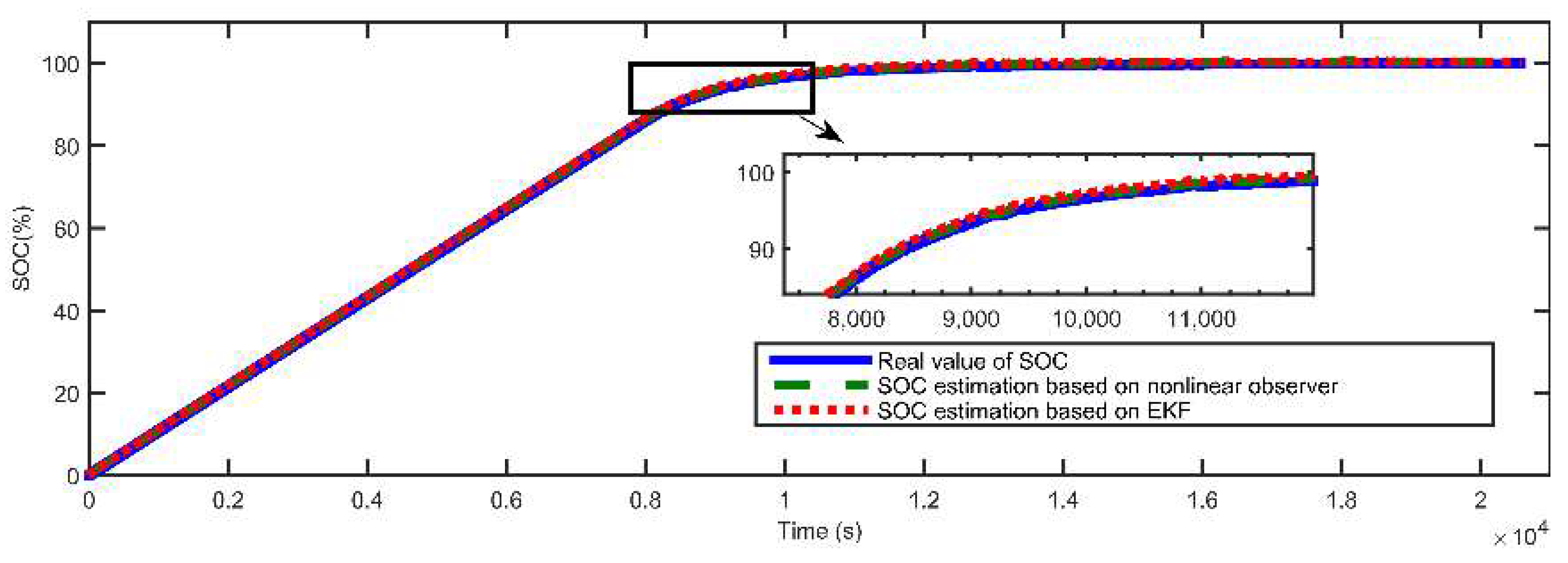
The results of estimating SOC using the proposed RBF neural network non-linear observer and EKF method are shown in Figure 11. It can be seen that the proposed RBF neural network non-linear observer accurately estimated the SOC. The error between the true value and the estimated value decreased gradually. The final estimated curve converged gradually near the true value curve, and the SOC error was limited to a very narrow error range. It was related to accurately modeling and accurately estimating the battery end voltage, which was used to correct the estimated SOC. Furthermore, this proved that the identified fractional-order electrochemical impedance model could accurately capture the battery dynamics and accurately estimate the battery end voltage, thus enabling the designed RBF neural network, non-linear, fractional-order observer to accurately and effectively estimate the SOC and power in batteries.

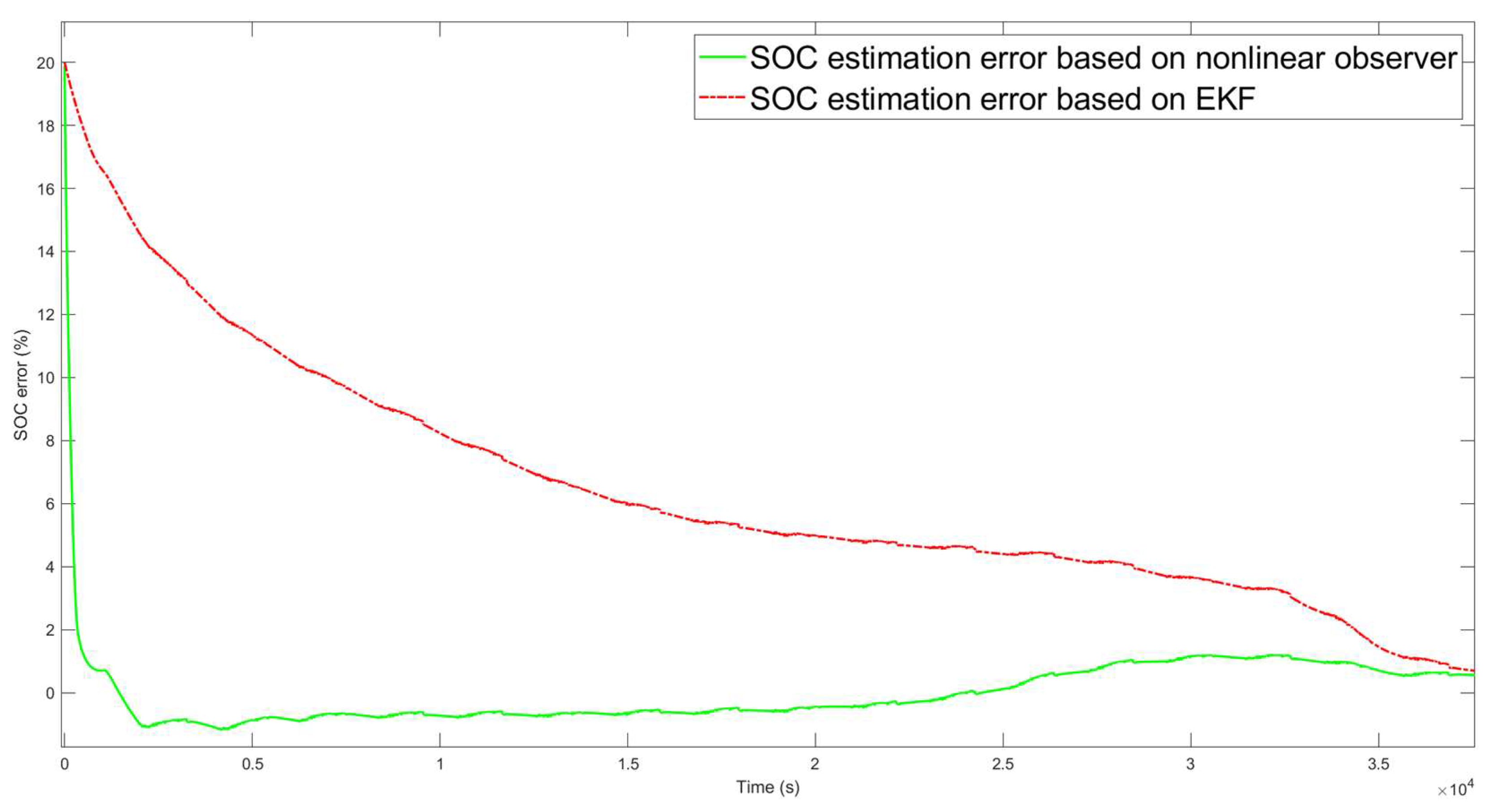
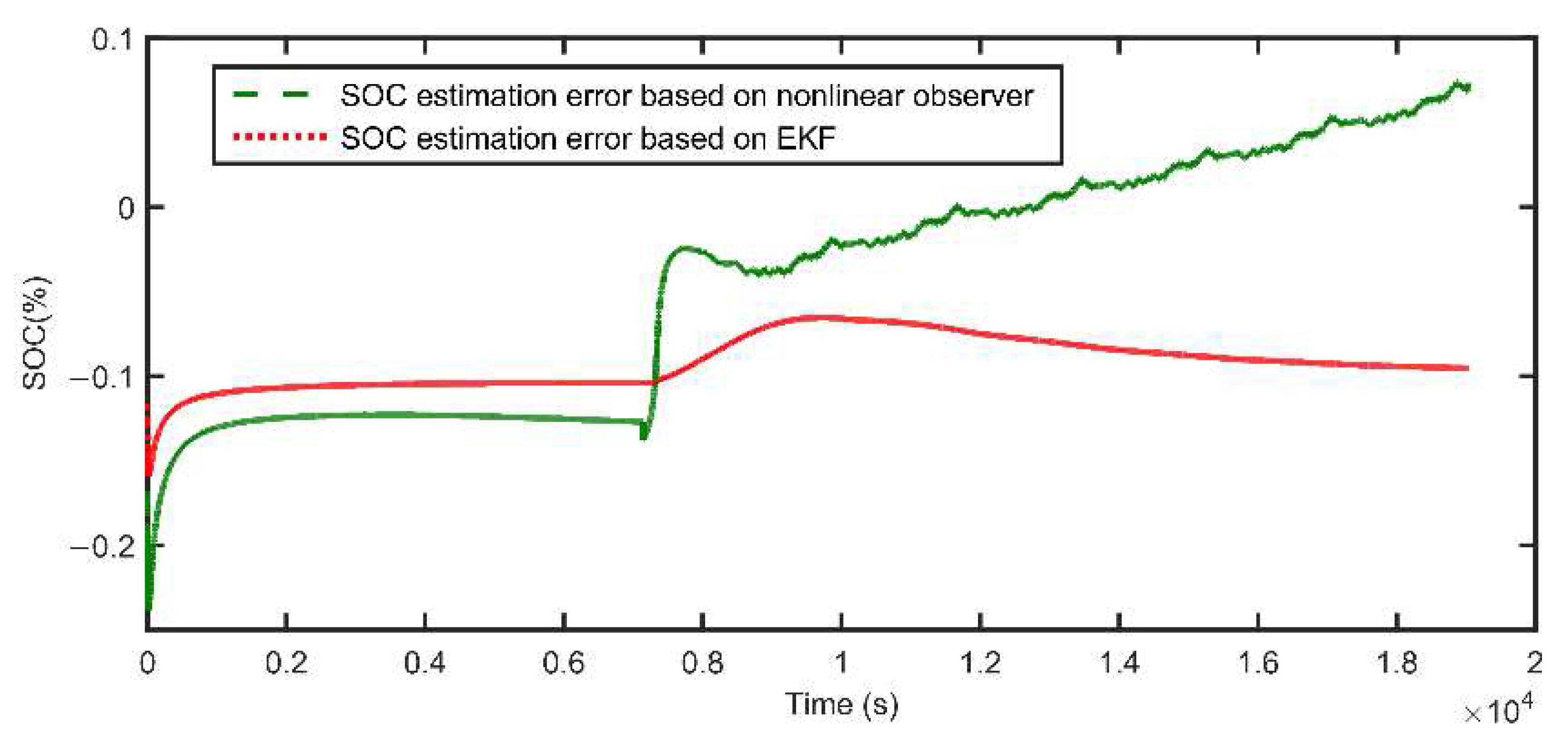
In order to compare the error of SOC estimation between the two methods, the error of SOC state estimation is also shown in Figure 12. The curve of the proposed RBF neural network non-linear observer SOC estimation error was nearly zero, and SOC error mainly fluctuated within the range of +0.5%. Conversely, SOC estimation error based on EKF method varied greatly, and the error range was large. The validity of the proposed RBF neural network non-linear observer is further proved.

In practical engineering applications, the ability to correct SOC is necessary for a good SOC estimation algorithm. Therefore, in the case of dynamic condition 1, the strategy of random SOC initial value was adopted to verify the SOC correction ability of the proposed algorithm. As shown in Figure 13 and Figure 14, when the initial SOC value deviated from the real value, the RBF neural network non-linear observer could quickly converge to the true value in a short time and keep the error below 2%, while the EKF method converged to the true value almost at the end of the test. The convergence speed of the proposed RBF neural network non-linear observer is further proved.

Remark 3.

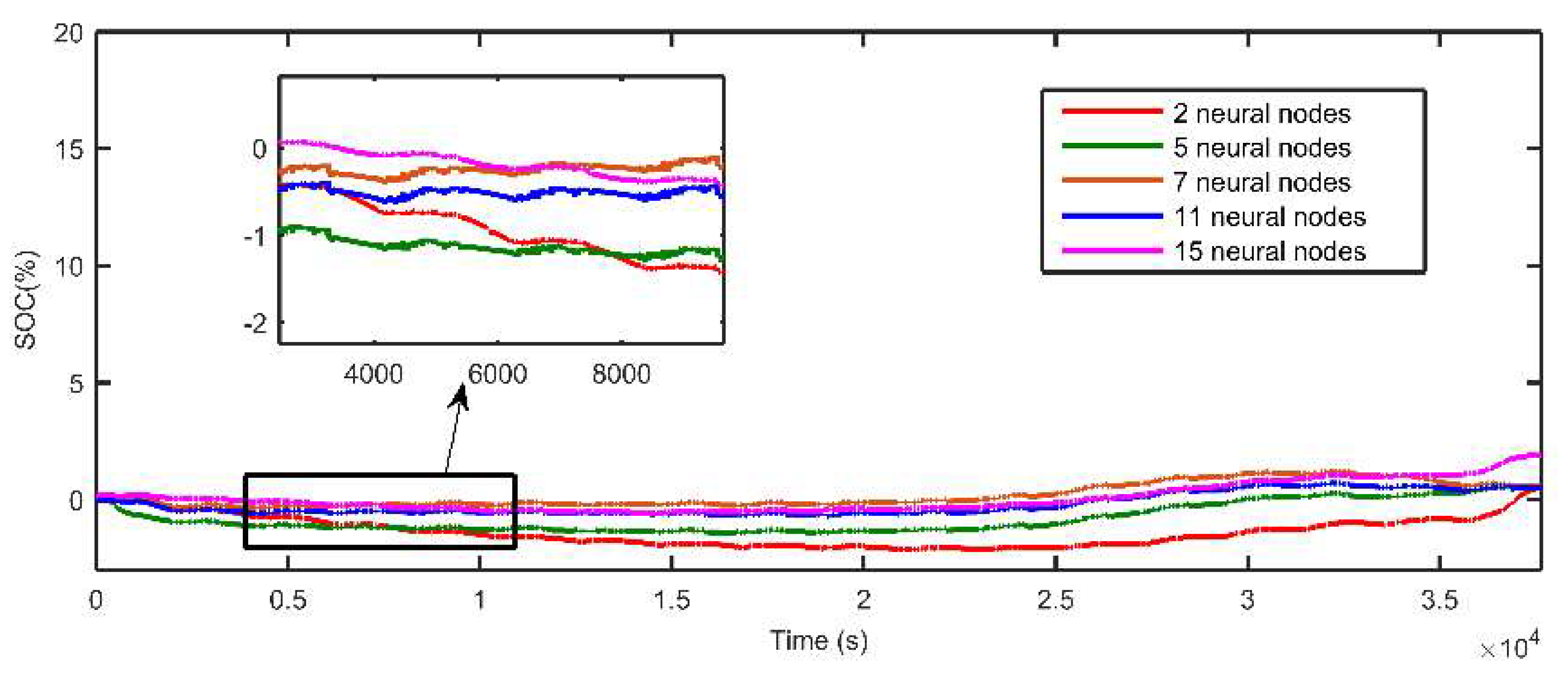
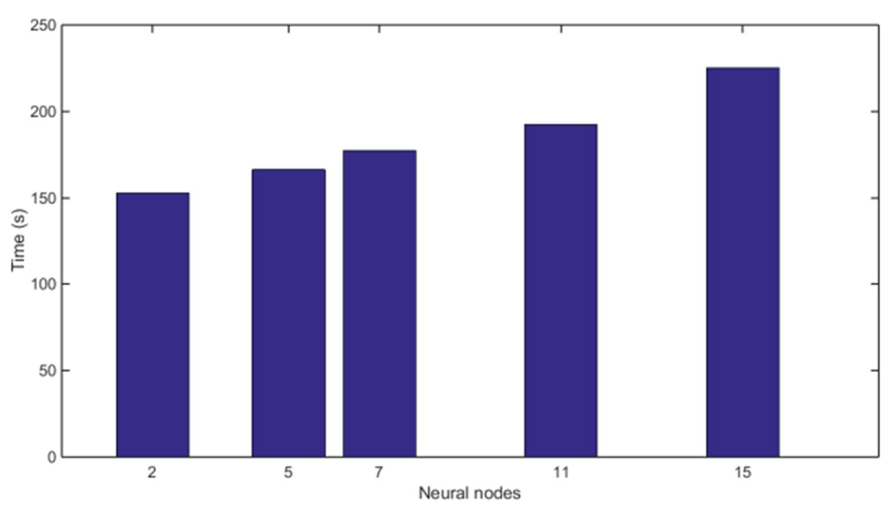
The effects of the number of ganglion points on the performance and calculation of SOC estimation for lithium-ion power batteries based on an RBF neural network non-linear observer were studied through comparative experiments and simulations. More specifically, two, five, seven, eleven and fifteen lithium-ion power batteries were compared to estimate their SOC performance and load using the experimental data of battery current and end voltage collected. The performance comparison of the RBF neural network non-linear observers with different ganglion points for estimating SOC is shown inFigure 15. The running time for solving the non-linear observer problem of RBF neural networks with different number of ganglion points is shown inFigure 16to represent the computational burden of different ganglion points. From the comparison results, the neural network non-linear observer used in the experiment with seven ganglion points has good performance under a reasonable amount of calculation.

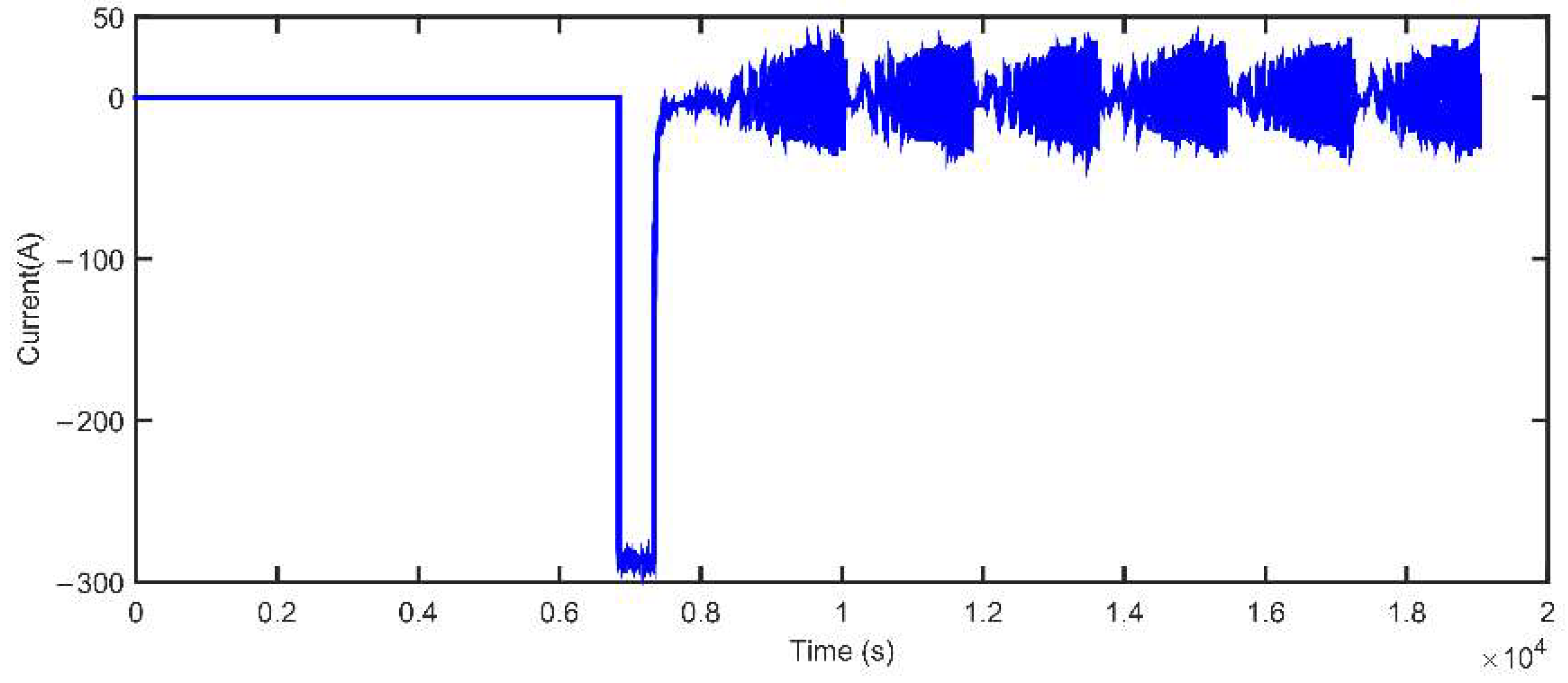
Dynamic operation test 2: Leave the fully charged battery in the incubator for 24 h at the laboratory temperature to ensure that the temperature of the whole battery is even. The battery is charged to full capacity with a constant current of 1C, and then tested under dynamic condition 2. When fully charged, the battery is discharged with high current for a period, and then charged and discharged with the current changing with dynamic fluctuations. The current image of dynamic condition test 2 is shown in Figure 17.

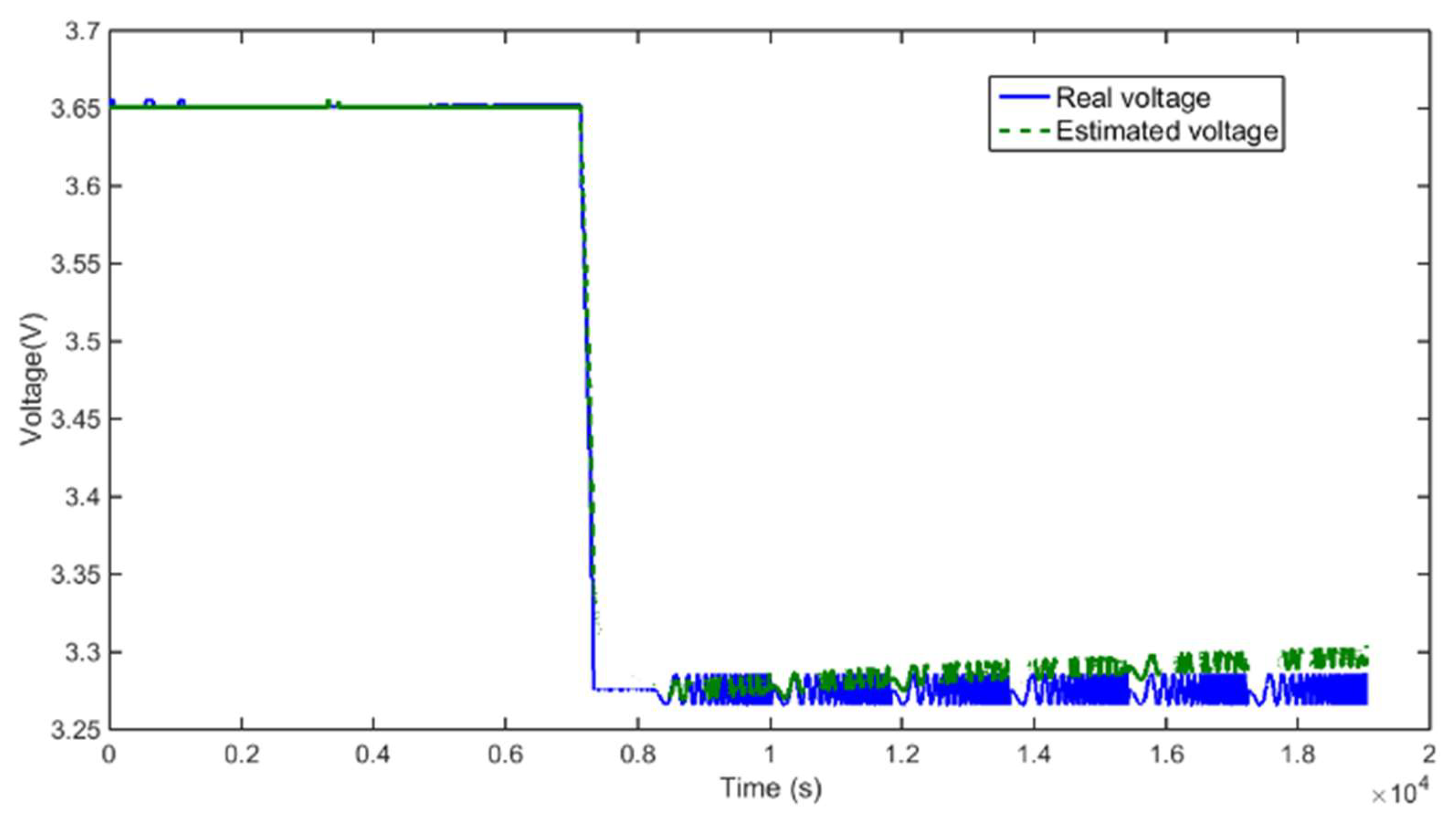
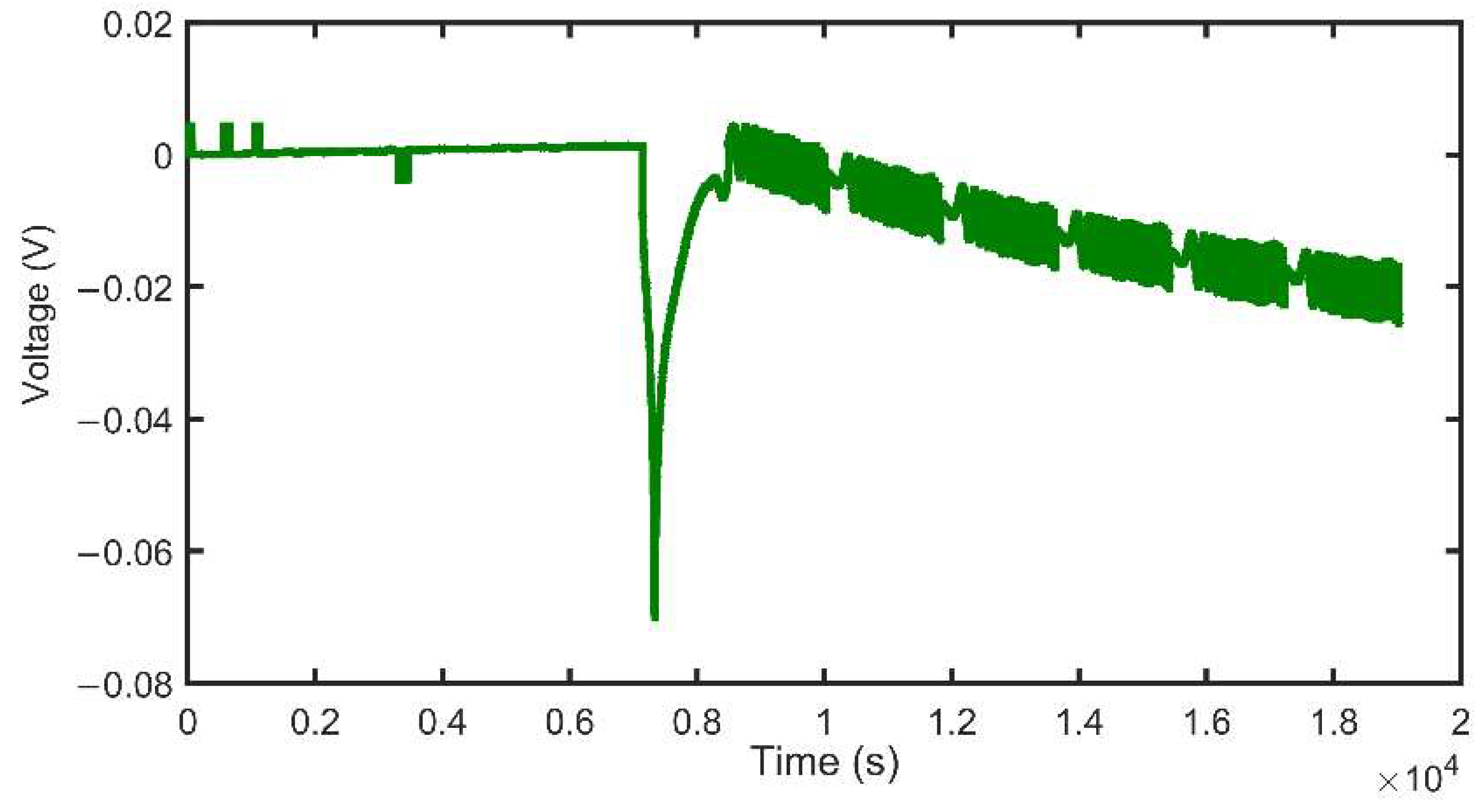
The measured actual end voltage used for reference and the model estimated end voltage curve are shown in Figure 18. It can be seen that the measured actual end voltage curve used for reference and the curve estimated by the model did not coincide as in Working Condition 1. The main reason for this is that the voltage fluctuation in the second half of the test was so small that the model did not track the voltage change in the power battery very accurately. The corresponding voltage error curves are shown in Figure 19. The RMSE of the true and model results was 11.7 mV under the dynamic condition test 2. This indicates that the model was less accurate under very small voltage fluctuations, but the accuracy of the estimation was still high enough.

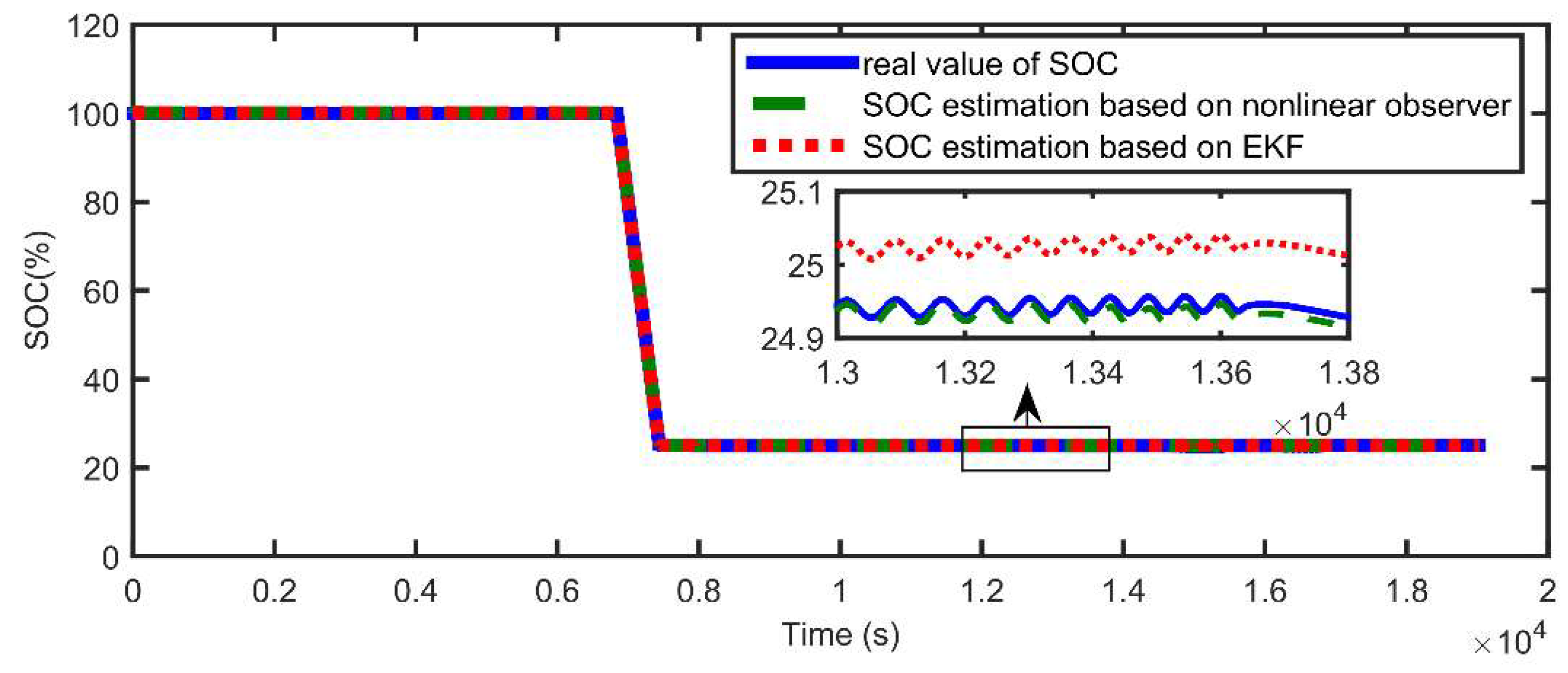
The results of estimating SOC using the proposed RBF neural network non-linear observer and the EKF method are shown in Figure 20. The error of estimating SOC state using the proposed RBF neural network non-linear observer and the EKF method is shown in Figure 21. It can be seen that the proposed RBF neural network non-linear observer accurately estimated the SOC of power batteries, and the estimated SOC error decreased gradually. However, due to the small fluctuation of voltage in the second half of the test period, the SOC estimation error did not converge to a range gradually because the model did not track the change in power battery end voltage very accurately. However, it can be seen from Figure 21 that the SOC estimation curve of the proposed non-linear observer of the RBF neural network was still very close to the real value of SOC. On the contrary, although the SOC estimation curve obtained using the EKF method was closer to the true value in the early stage, the error increased during the back-end test process. The proposed RBF neural network non-linear observer was more accurate than the EKF method.

Dynamic operation test 3: Leave the fully charged battery in the incubator for 26 h at the laboratory temperature to ensure that the temperature of the whole battery is even. Charge the battery to its full capacity using a constant current of 1C and discharge it to zero power battery capacity. Test under dynamic condition 3, charge the battery with a high current for a period after discharging, and then charge and discharge with dynamic fluctuating current. The image of the current under dynamic condition test 2 is shown in Figure 22.

The measured actual end voltage for the reference and the model-estimated end voltage curve are shown in Figure 23. The measured actual end voltage curve coincided with the model estimated curve. The corresponding voltage error curve is shown in Figure 24. The RMSE of the real and model results was 9.69 mV under dynamic condition test 3, which indicates that the proposed electrochemical impedance model could accurately estimate the terminal voltage of the power battery.

The results of estimating SOC using the proposed RBF neural network non-linear observer and the EKF method are shown in Figure 25. It can be seen that the proposed RBF neural network non-linear observer accurately estimated the SOC, and the error between the true value and the estimated value was small. The SOC state estimation error estimated using the proposed RBF neural network non-linear observer and the EKF method is shown in Figure 26. It can be observed that the SOC estimation error curve of the proposed RBF neural network non-linear observer was closer to the transverse coordinate axis. Although the SOC error curve estimated using the EKF method decreased gradually at the end, the SOC estimation error was larger in the middle of the curve. The accuracy of the proposed non-linear observer for RBF neural networks is further demonstrated.

To further show the accuracy of the proposed RBF neural network non-linear observer in estimating the SOC of the EKF method,

Table 2. RMSE of SOC estimation error based on RBF neural network non-linear observer and EKF method.

	Working Condition 1	Working Condition 2	Working Condition 3
RBF neural network non-linear observer	0.53%	0.24%	0.33%
EKF method	1.42%	1.70%	0.75%

gives the RMSE results of estimating the SOC using the proposed RBF neural network non-linear observer and the EKF method under three dynamic operating conditions tests. Figure 12, Figure 21 and Figure 26 and Table 2 show that the RBF non-linear observer designed has higher estimation accuracy than the EKF.

The comparison of the accuracy of the EKF method with the RBF neural network non-linear observer proposed under different dynamic test conditions is given. The following are the simulation results of voltage and SOC estimation using the proposed RBF neural network non-linear observer under dynamic test condition 1 under integer- and fractional-order models.

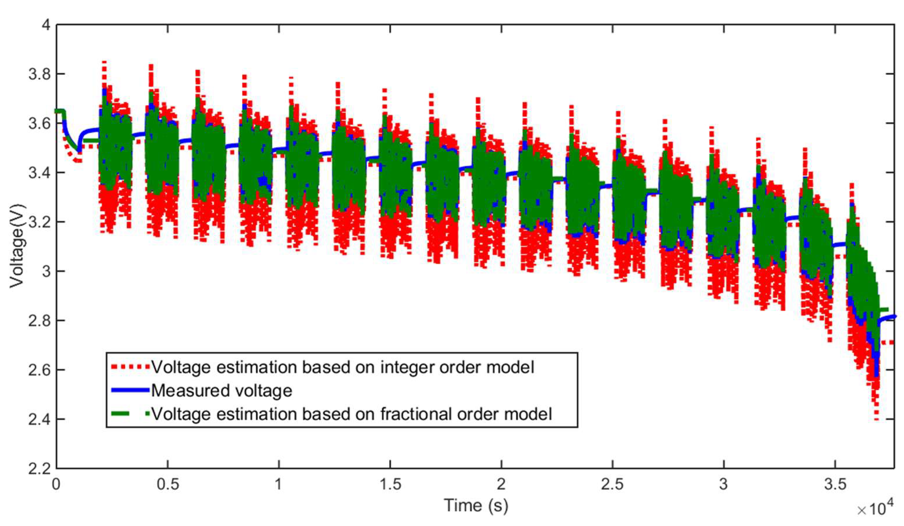
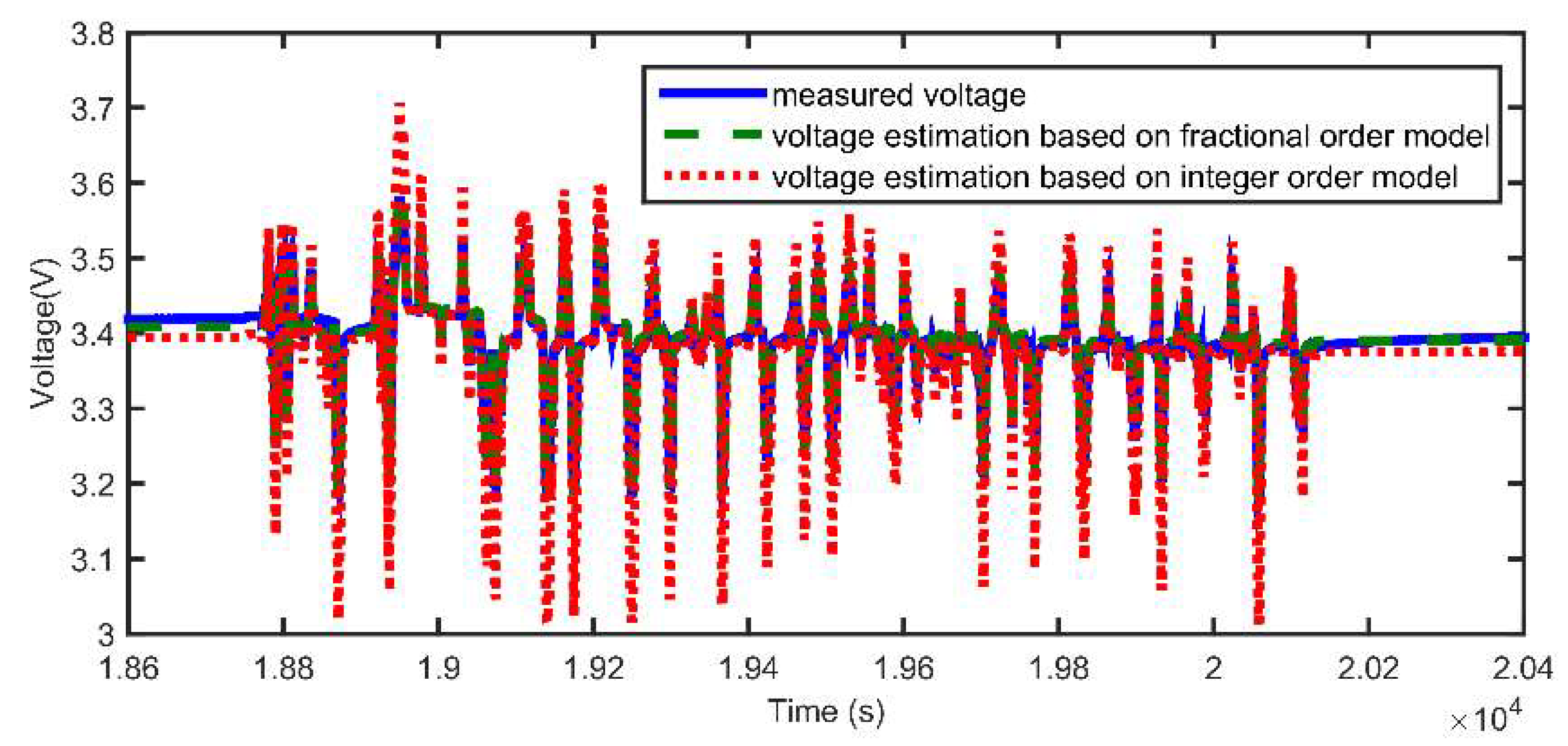
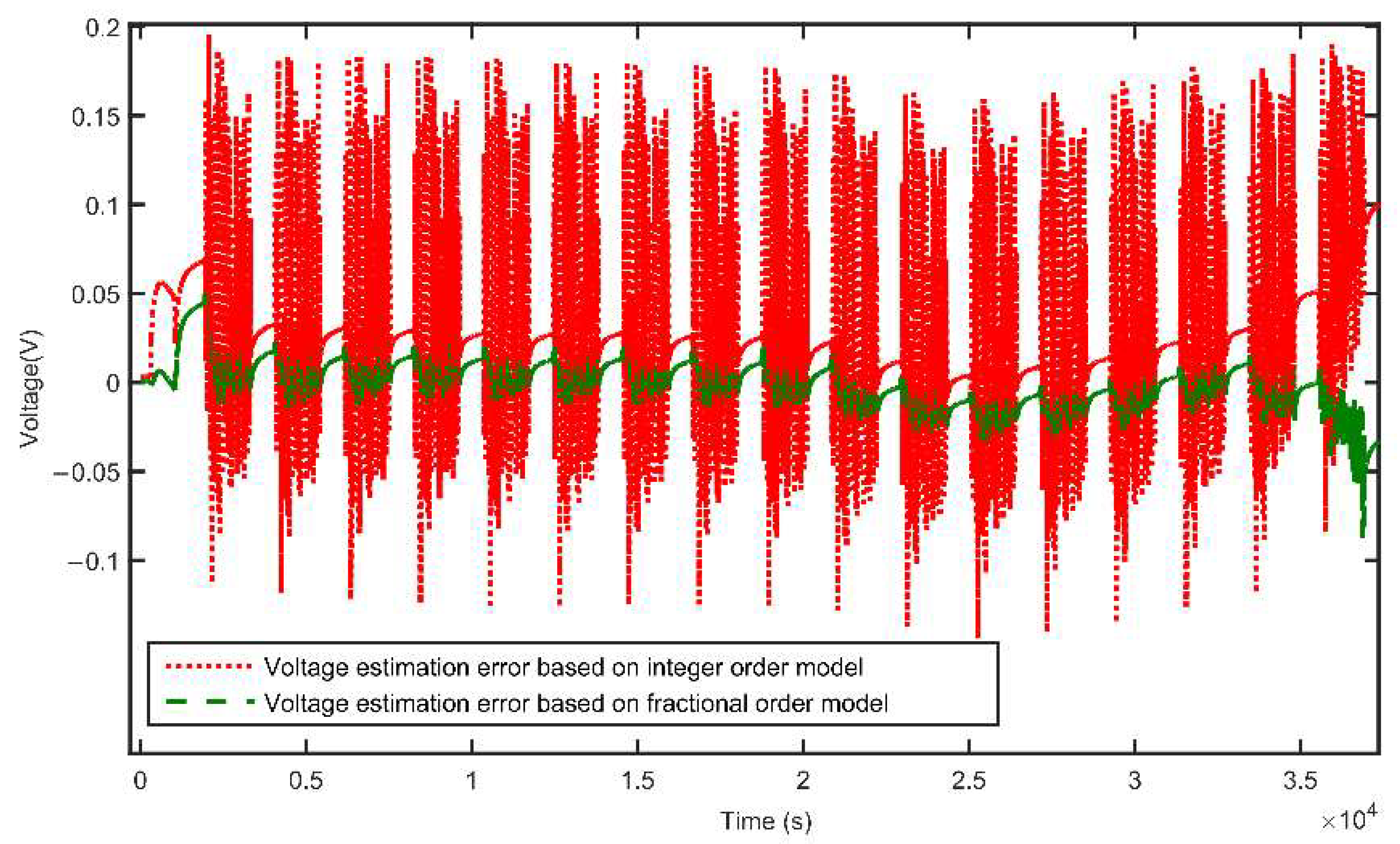
Figure 27 shows the estimation of battery end voltage using the integer-order model and the proposed electrochemical impedance fractional-order model, the actual measured end voltage, and the comparison of the estimated end voltage curves between the two models. Figure 28 shows the local amplification comparison of the two models, and the corresponding voltage error curves are shown in Figure 29. The local magnification diagram shown in Figure 28 shows that the measured actual end voltage curve used for reference coincides basically with the curve estimated based on the fractional model of electrochemical impedance, while the voltage estimate based on the integer-order model has a greater error than that based on the fractional-order model. The RMSE based on fractional-order model voltage estimation was 5.97 mV, and 13.7 mV based on integer-order model voltage estimation. This shows that the proposed fractional-order model of electrochemical impedance for power batteries can clearly reflect its dynamic characteristics and battery performance.

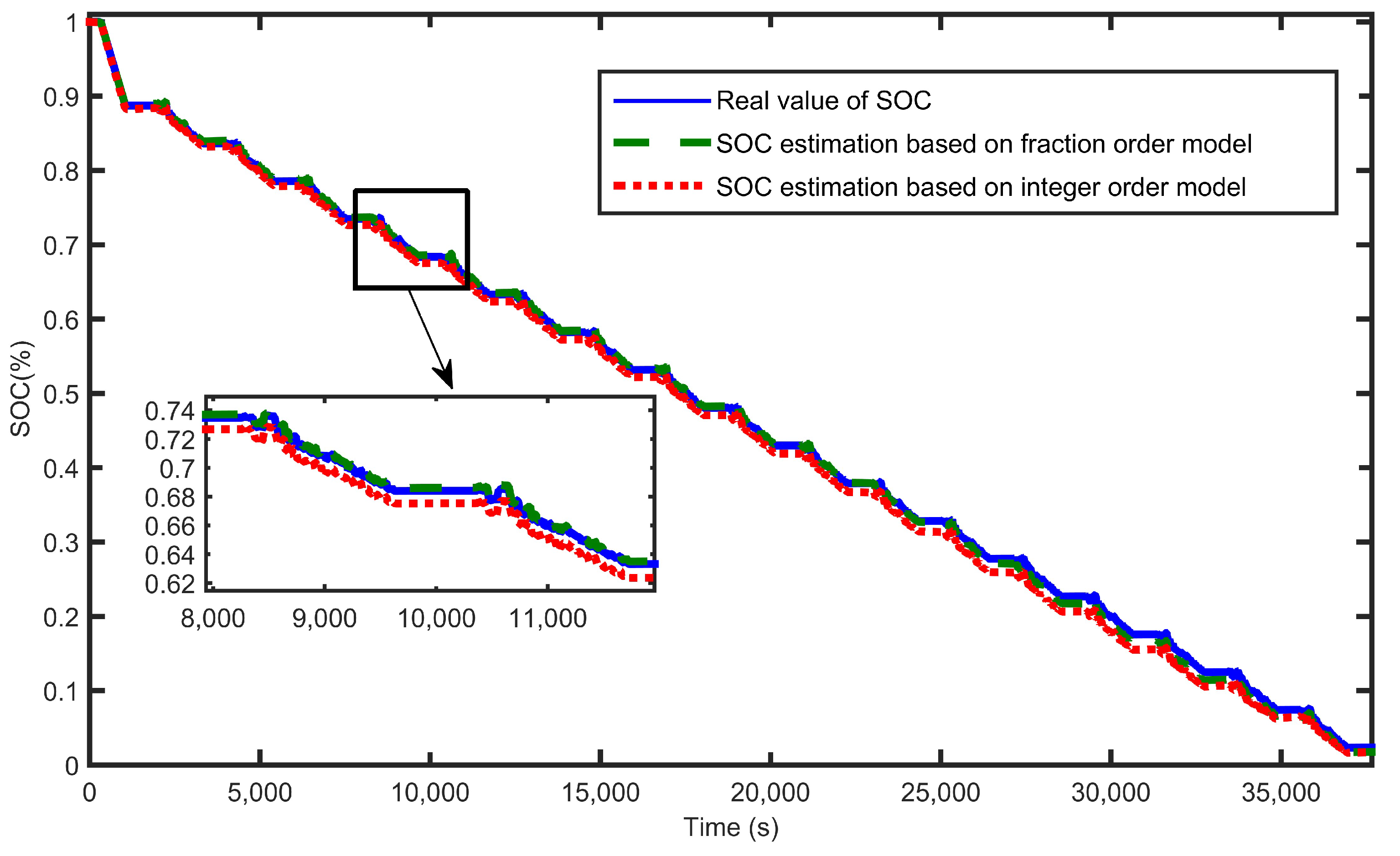
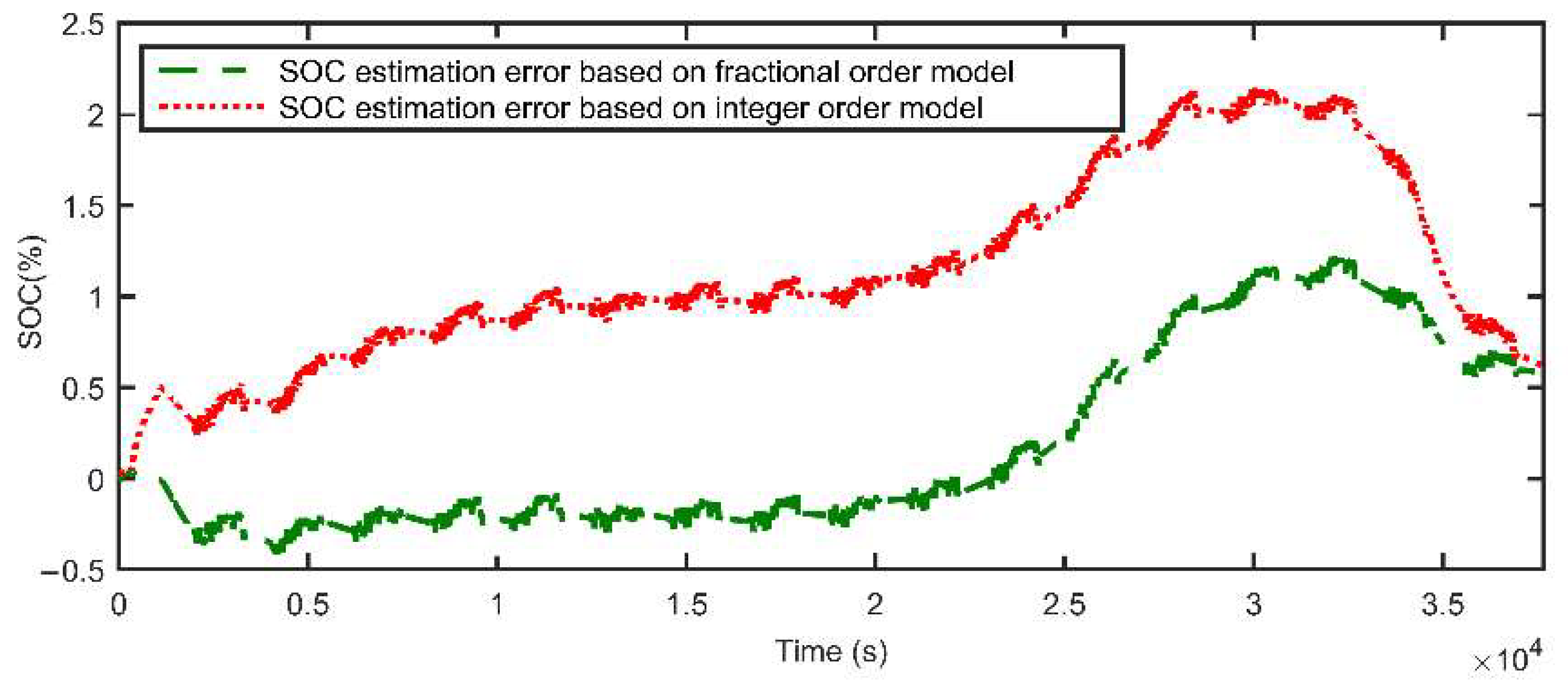
The proposed non-linear observer of the RBF neural network was used to estimate SOC based on the fractional- and integer-order models of electrochemical impedance proposed. The estimation curve of SOC is shown in Figure 30. From Figure 30, it can be seen that the SOC estimation curve of the fractional electrochemical impedance model proposed basically coincided with the true value curve, and the estimation result was better than that based on the integer-order model. The RMSE of SOC based on the fractional model of electrochemical impedance was 0.53%, and that of SOC based on the integer model was 1.26%.Using the proposed RBF neural network non-linear observer to estimate SOC based on the proposed fractional and integer-order models, the results show that the estimated SOC error based on the fractional-order model of electrochemical impedance was between (+) 0.5% and that based on the integer-order model was between 0.5% and 2%.The proposed fractional model of electrochemical impedance can more accurately estimate the SOC of power batteries.

The following conclusions can be drawn from the above experimental simulation results in Figure 11, Figure 12, Figure 20, Figure 21, Figure 25, Figure 26, Figure 30 and Figure 31 and Table 1:

(1)

From Figure 30 and Figure 31, the proposed non-linear observer of RBF neural network has higher accuracy in estimating SOC of the fractional-order model of electrochemical impedance than that of the integer-order model, because the proposed fractional-order model of electrochemical impedance has smaller modeling error, more accurate estimation of end voltage of power batteries and less error in estimating the SOC state of batteries.

(2)

For power battery SOC estimation, the proposed RBF-neural-network-based non-linear observer has smaller error and higher accuracy than the EKF method. From Figure 11, Figure 20 and Figure 25, the curve of SOC estimation using the EKF method is smoother than that of the proposed RBF neural network non-linear observer. The reason for these two phenomena is that the observer-based method is superior to the filter in estimating the system output. The observer-based non-linear observer based on the RBF neural network can quickly catch the change when the experimental current changes significantly between positive and negative modes in three dynamic operating conditions. The convergence rate of state estimation is then adjusted.

(3)

From Figure 12, Figure 21 and Figure 26, it can be seen that the proposed non-linear observer method for RBF neural networks converges faster than the EKF in SOC state estimation. The RMSE of the SOC estimation errors for the two methods in Table 1 further demonstrates that the proposed non-linear observer method for RBF neural networks is superior to the EKF method.

Based on the above analysis, it is known that the fractional model of electrochemical impedance proposed has less modeling error and higher estimation accuracy than the integer model. For the fractional-order model of electrochemical impedance proposed, the proposed RBF neural network non-linear observer method is more effective and more accurate than the EKF method. The proposed RBF neural network non-linear observer method can run in real time and reliably and accurately estimate the end voltage and SOC state of power batteries. In summary, the fractional-order model of electrochemical impedance and the RBF neural network non-linear observer method proposed not only take into account the characteristics of the battery itself, but also show good performance.

5. Conclusions

This paper designed a method for the state of charge (SOC) estimation of lithium-ion batteries based on an electrochemical impedance equivalent circuit model with a controlled source. A non-linear observer was designed to estimate the SOC of batteries by using an RBF neural network to estimate the uncertainty of batteries online. The estimation error of the non-linear observer based on an RBF neural network was proved to be ultimately bounded by Lyapunov stability analysis. The results of simulations and experiments in this paper are as follows: compared with the EKF, the average error of SOC measurement with the non-linear observer was reduced by 50%, and the error of the optimal experimental result was reduced by 70%. Compared with the integer-order model, the measurement error of the fractional-order model was reduced by 40% on average, and the error of the optimal experimental result was reduced by 60%. The experimental and simulation results show the accuracy and superiority of the proposed method.

References

- Wachtmeister, M. Overview and Analysis of Environmental and Climate Policies in China’s Automotive Sector. J. Environ. Dev. 2013, 22, 284–312. [Google Scholar] [CrossRef]
- Hu, X.; Li, S.E.; Yang, Y. Advanced Machine Learning Approach for Lithium-Ion Battery State Estimation in Electric Vehicles. IEEE Trans. Transp. Electrif. 2015, 2, 140–149. [Google Scholar] [CrossRef]
- Xiong, R.; Zhang, Y.; He, H.; Zhou, X.; Pecht, M.G. A Double-Scale, Particle-Filtering, Energy State Prediction Algorithm for Lithium-Ion Batteries. IEEE Trans. Ind. Electron. 2017, 65, 1526–1538. [Google Scholar] [CrossRef]
- Xiong, R.; Yu, Q.; Wang, L.Y.; Lin, C. A novel method to obtain the open circuit voltage for the state of charge of lithium ion batteries in electric vehicles by using H infinity filter. Appl. Energy 2017, 207, 346–353. [Google Scholar] [CrossRef]
- Xiong, R.; Li, L.; Tian, J. Towards a smarter battery management system: A critical review on battery state of health monitoring methods. J. Power Source 2018, 405, 18–29. [Google Scholar] [CrossRef]
- Wang, Y.; Zhang, C.; Chen, Z. A method for joint estimation of state-of-charge and available energy of LiFePO4 batteries. Appl. Energy 2014, 135, 81–87. [Google Scholar] [CrossRef]
- Moura, S.J.; Chaturvedi, N.A.; Krstić, M. Adaptive Partial Differential Equation Observer for Battery State-of-Charge/State-of-Health Estimation Via an Electrochemical Model. J. Dyn. Syst. Meas. Control 2013, 136, 011015. [Google Scholar] [CrossRef]
- Ng, K.S.; Moo, C.-S.; Chen, Y.-P.; Hsieh, Y.-C. Enhanced coulomb counting method for estimating state-of-charge and state-of-health of lithium-ion batteries. Appl. Energy 2009, 86, 1506–1511. [Google Scholar] [CrossRef]
- Javid, G.; Abdeslam, D.O.; Basset, M. Adaptive Online State of Charge Estimation of EVs Lithium-Ion Batteries with Deep Recurrent Neural Networks. Energies 2021, 14, 758. [Google Scholar] [CrossRef]
- Liu, Y.; Li, J.; Zhang, G.; Hua, B.; Xiong, N. State of Charge Estimation of Lithium-Ion Batteries Based on Temporal Convolutional Network and Transfer Learning. IEEE Access 2021, 9, 34177–34187. [Google Scholar] [CrossRef]
- Shen, Y. Adaptive online state-of-charge determination based on neuro-controller and neural network. Energy Convers. Manag. 2010, 51, 1093–1098. [Google Scholar] [CrossRef]
- Chen, M.; Rincon-Mora, G.A. Accurate Electrical Battery Model Capable of Predicting Runtime and I–V Performance. IEEE Trans. Energy Convers. 2006, 21, 504–511. [Google Scholar] [CrossRef]
- Chen, N.; Zhang, P.; Dai, J.; Gui, W. Estimating the State-of-Charge of Lithium-Ion Battery Using an H-Infinity Observer Based on Electrochemical Impedance Model. IEEE Access 2020, 8, 26872–26884. [Google Scholar] [CrossRef]
- Liu, C.; Liu, W.; Wang, L.; Hu, G.; Ma, L.; Ren, B. A new method of modeling and state of charge estimation of the battery. J. Power Source 2016, 320, 1–12. [Google Scholar] [CrossRef]
- Liu, Z.; Qiu, Y.; Feng, J.; Chen, S.; Yang, C. A simplified fractional order modeling and parameter identification for lithium-ion batteries. J. Electrochem. Energy Convers. Storage 2022, 19, 021001. [Google Scholar] [CrossRef]
- Li, J.; Wang, L.; Lyu, C.; Liu, E.; Xing, Y.; Pecht, M. A parameter estimation method for a simplified electrochemical model for Li-ion batteries. Electrochim. Acta 2018, 275, 50–58. [Google Scholar] [CrossRef]
- Hu, M.; Li, Y.; Li, S.; Fu, C.; Qin, D.; Li, Z. Lithium-ion battery modeling and parameter identification based on fractional theory. Energy 2018, 165, 153–163. [Google Scholar] [CrossRef]
- Xiong, R.; Tian, J.; Mu, H.; Wang, C. A systematic model-based degradation behavior recognition and health monitoring method for lithium-ion batteries. Appl. Energy 2017, 207, 372–383. [Google Scholar] [CrossRef]
- Mawonou, K.S.; Eddahech, A.; Dumur, D.; Beauvois, D.; Godoy, E. Improved state of charge estimation for Li-ion batteries using fractional order extended Kalman filter. J. Power Source 2019, 435, 226710. [Google Scholar] [CrossRef]
- Plett, G. Extended Kalman filtering for battery management systems of LiPB-based HEV battery packs: Part 1. Background. J. Power Source 2004, 134, 252–261. [Google Scholar] [CrossRef]
- Jiang, Z.; Shi, Q.; Wei, Y.; Wei, H.; Gao, B.; He, L. An Immune Genetic Extended Kalman Particle Filter approach on state of charge estimation for lithium-ion battery. Energy 2021, 230, 120805. [Google Scholar]
- Xiaosong, H.; Fengchun, S.; Zou, Y. Estimation of State of Charge of a Lithium-Ion Battery Pack for Electric Vehicles Using an Adaptive Luenberger Observer. Energies 2010, 3, 1586–1603. [Google Scholar]
- Xu, J.; Mi, C.; Cao, B.; Deng, J.; Chen, Z.; Li, S. The State of Charge Estimation of Lithium-Ion Batteries Based on a Proportional-Integral Observer. IEEE Trans. Veh. Technol. 2014, 63, 1614–1621. [Google Scholar] [CrossRef]
- Zhang, F.; Liu, G.; Fang, L. Estimation of Battery State of Charge with H infinity Observer: Applied to a Robot for Inspecting Power Transmission Lines. IEEE Trans. Ind. Electron. 2012, 59, 1086–1095. [Google Scholar] [CrossRef]
- Zhang, Y.; Zhang, C.; Zhang, X. State-of-charge estimation of the lithium-ion battery system with time-varying parameter for hybrid electric vehicles. IET Control. Theory Appl. 2014, 8, 160–167. [Google Scholar] [CrossRef]
- Kim, I.-S. The novel state of charge estimation method for lithium battery using sliding mode observer. J. Power Source 2006, 163, 584–590. [Google Scholar] [CrossRef]
- Chen, X.; Shen, W.; Dai, M.; Cao, Z.; Jin, J.; Kapoor, A. Robust Adaptive Sliding-Mode Observer Using RBF Neural Network for Lithium-Ion Battery State of Charge Estimation in Electric Vehicles. IEEE Trans. Veh. Technol. 2016, 65, 1936–1947. [Google Scholar] [CrossRef]
- Kim, I.-S. Nonlinear State of Charge Estimator for Hybrid Electric Vehicle Battery. IEEE Trans. Power Electron. 2008, 23, 2027–2034. [Google Scholar] [CrossRef]
- Wang, Y.; Zhang, C.; Chen, Z. A method for state-of-charge estimation of LiFePO4 batteries at dynamic currents and temperatures using particle filter. J. Power Source 2015, 279, 306–311. [Google Scholar] [CrossRef]
- Li, J.; Barillas, J.K.; Guenther, C.; Danzer, M.A. Multicell state estimation using variation based sequential Monte Carlo filter for automotive battery packs. J. Power Source 2015, 277, 95–103. [Google Scholar] [CrossRef]
- Charkhgard, M.; Farrokhi, M. State-of-Charge Estimation for Lithium-Ion Batteries Using Neural Networks and EKF. IEEE Trans. Ind. Electron. 2011, 57, 4178–4187. [Google Scholar] [CrossRef]
- Chen, Z.; Fu, Y.; Mi, C. State of Charge Estimation of Lithium-Ion Batteries in Electric Drive Vehicles Using Extended Kalman Filtering. IEEE Trans. Veh. Technol. 2013, 62, 1020–1030. [Google Scholar] [CrossRef]
- Zhang, J.; Xia, C. State-of-charge estimation of valve regulated lead acid battery based on multi-state Unscented Kalman Filter. Int. J. Electr. Power Energy Syst. 2011, 33, 472–476. [Google Scholar] [CrossRef]
- Ouyang, Q.; Chen, J.; Wang, F.; Su, H. Nonlinear Observer Design for the State of Charge of Lithium-Ion Batteries. IFAC Proc. Vol. 2014, 47, 2794–2799. [Google Scholar] [CrossRef] [Green Version]
- Chen, B.; Zhang, H.; Lin, C. Observer-Based Adaptive Neural Network Control for Nonlinear Systems in Nonstrict-Feedback Form. IEEE Trans. Neural Netw. Learn. Syst. 2015, 27, 89–98. [Google Scholar] [CrossRef]
- Zhao, Z.; Ren, Y.; Mu, C.; Zou, T.; Hong, K.-S. Adaptive Neural-Network-Based Fault-Tolerant Control for a Flexible String with Composite Disturbance Observer and Input Constraints. IEEE Trans. Cybern. 2021, 1–11. [Google Scholar] [CrossRef]
- Chen, J.; Ouyang, Q.; Xu, C.; Su, H. Neural Network-Based State of Charge Observer Design for Lithium-Ion Batteries. IEEE Trans. Control Syst. Technol. 2017, 26, 313–320. [Google Scholar] [CrossRef]
- Petras, I. Fractional-Order Nonlinear Systems: Modeling, Analysis and Simulation; Springer Science & Business Media: Berlin/Heidelberg, Germany, 2011. [Google Scholar]
Figure 1.
Typical EIS of a lithium-ion battery.
Figure 2.
Electrochemical impedance circuit model of battery.
Figure 3.
Architecture diagram of battery characteristic test platform.
Figure 4.
Photos of battery characteristic test platform.
Figure 5.
Battery test system interface.
Figure 6.
(a) Relationship between OCV and SOC of battery. (b) Parameters of battery equivalent circuit model and its fitting curve.
Figure 7.
Current of dynamic condition test 1 experiment.
Figure 8.
Comparison of real and estimated voltage of test 1 under dynamic condition.
Figure 9.
Comparison of real value and estimated value of experimental terminal voltage in dynamic condition test 1.
Figure 10.
Voltage estimation error of experiment terminal in dynamic condition test 1.
Figure 11.
Comparison of SOC estimation based on non-linear observer and EKF in dynamic condition test 1.
Figure 12.
Comparison of SOC estimation error based on non-linear observer and EKF in dynamic condition test 1.
Figure 13.
Comparison of SOC estimation based on non-linear observer and EKF in dynamic condition test 1 under random SOC initial value.
Figure 14.
Figure 15.
SOC estimation error of non-linear observers with different numbers of neural nodes.
Figure 16.
Time consuming of solving non-linear observers with different numbers of neural nodes.
Figure 17.
Dynamic condition test 2 experimental current.
Figure 18.
Comparison of real and estimated voltage of test 2 under dynamic condition.
Figure 19.
Voltage estimation error of test 2 under dynamic condition.
Figure 20.
Comparison of SOC estimation based on non-linear observer and EKF in dynamic condition test 2.
Figure 21.
Comparison of SOC estimation error based on non-linear observer and EKF in dynamic condition test 2.
Figure 22.
Dynamic condition test 3 experimental current.
Figure 23.
Comparison of real and estimated voltage of test 3 under dynamic condition.
Figure 24.
Voltage estimation error of test 3 under dynamic condition.
Figure 25.
Comparison of SOC estimation based on non-linear observer and EKF in dynamic condition test 3.
Figure 26.
Comparison of SOC estimation error based on non-linear observer and EKF in dynamic condition test 3.
Figure 27.
Comparison of voltage estimation based on fractional-order model and integer-order model.
Figure 28.
Comparison and enlargement of voltage estimation based on fractional-order model and integer-order model.
Figure 29.
Comparison of voltage estimation error based on fractional-order model and integer-order model.
Figure 30.
Comparison of SOC estimates based on fractional-order model and integer-order model.
Figure 31.
Comparison of SOC estimation error based on fractional-order model and integer-order model.