
Design and Modelling of Energy Conversion with the Two-Region Torque Control of a PMSM in an EV Powertrain


1
Department of Power Electronics and Energy Control Systems, AGH University of Science and Technology, 30-059 Kraków, Poland
2
Department of Electrical Engineering, Polytechnic Faculty, University of Applied Sciences in Tarnow, 33-100 Tarnów, Poland
*
Author to whom correspondence should be addressed.
Energies 2022, 15(13), 4887; https://0-doi-org.brum.beds.ac.uk/10.3390/en15134887
Submission received: 14 May 2022
/
Revised: 21 June 2022
/
Accepted: 30 June 2022
/
Published: 3 July 2022
(This article belongs to the Special Issue Electric Vehicles Power Train, Storage and Charging: Design, Modelling and Simulation)
Abstract
:This paper investigates the properties and design of energy conversion in an electric vehicle (EV) powertrain. Here, we combined the dynamics of vehicle motion with controlled electric propulsion, which is an EV powertrain. The control of two types of permanent magnet synchronous motors (PMSMs) was considered. An algorithm was developed for the determination of the static characteristics of two-region motor torque control. A constant torque and a constant power region were used in the powertrain of the EV. The design of the control system for the PMSM was considered in the reference frame. A precise mechanical model of the EV and the determination of road loads is shown. The main results of this study were the selection of the PI controller parameters (in analytical form), which was carried out for the simplified motor model and then extended for the model, and energy consumption during the WLTP standard driving cycle. The presented simulation results of the proposed control system with synchronous motors in the EV (Fisker Karma as an example) confirmed the approach taken for the selection of the controller. The presentation of the EV’s acceleration for an optimized powertrain, and hence its performance, is a novelty not found in other articles.
1. Introduction
This paper presents a performance assessment of a battery-powered electric vehicle employing a PMSM powertrain system from the electric motor to the WLTP (world harmonized light-duty vehicles test procedure) for electric vehicles.
The conversion of energy from electrical to mechanical is now the most important form of energy conversion, as most industry systems and modern vehicles are based on electric motors. EVs are now some of the most modern energy conversion systems and the automation of their drive motors is important. This article belongs thematically to the Energies Special Issue “Automation and Robotics Application in Energy Systems”.
Motor vehicles use mostly permanent magnet synchronous motors (PMSMs). They are used in vehicles (hybrid electric vehicles (HEVs) or electric vehicles (EVs)) from the following car manufacturers: Toyota (Lexus), Nissan, Renault, BMW, and Honda. These motors are characterized by high overload (no brushes, power loss mainly in the stator, and the possibility of effective cooling due to negligible electrical losses in the rotor), high dynamics resulting from the low moment of inertia of the rotor, high efficiency, and high power density and width of the rotational speed range. The negative properties of these motors are their high price and low—compared to induction motors—operating temperatures. However, despite this, their applications in industrial and automotive drives are increasing rapidly [1,2,3].
Manufactured PMSMs may differ in the shape and location of magnets in the rotor. In the case of electric vehicles in particular, they are used with interior magnets (interior permanent magnet synchronous motor, IPMSM) or with surface magnets (surface mount permanent magnet synchronous motor, SMPMSM). IPMSMs usually have higher stator inductances, and their rotors have magnetic asymmetry [3].
Two-region control of the motor: constant torque and constant power (field weakening control) were analyzed in [4,5,6,7,8], where the greatest focus was on the second zone of IPMSM control. This is because of the double-track control: the stator linked flux ( current) and the motor torque.
The analysis of two-region control leads to different control structures, but they are always vector methods in the () frame. A field-weakening operation based on feedback linearization is presented in [9]. A variable q-axis voltage control and voltage angle control (VAC) method is shown in [10]. The authors of [11] describe a decoupling system like that of induction motor control systems (field-oriented control). Ref. [12] focuses on the control of one PMSM construction: a segmented interior permanent magnet synchronous motor.
Previously cited works [4,5,6,7,8] have also developed control methods, usually a cascade control of the angular speed. The field-weakening algorithm for IPMSM was studied in [4], where only the motor was considered. In [5], as in the previously discussed paper, the greatest emphasis was placed on the mechanical characteristics realized for different flux-weakening methods. Ref. [6] also focused on weakened flux performance characteristics, with the addition of simulations of dynamic motor states. Complementary computational and simulation studies on PMSMs in the form of experimental results are included in [7,8]; however, these are general studies not dedicated to EVs.
While the titles of some articles include “EV”, many are just descriptions of control methods that do not take into account vehicle dynamics. Additionally, they omit the operation of the motor for constant power: These methods include state feedback decoupling control with disturbance feed-forward [13], where the extended Kalman filter is used, and the practical implementation of direct torque control (DTC), presented in Ref. [14]. In other words, these are methods that are suitable for motors in the 1/4–1/3 range of maximum vehicle speed. These articles include tests and experimental setups, meaning they are valuable and reliable, but are they for EVs? That is the question.
Other articles that include “EV” in the title are detailed descriptions of two-region control methods; however, they do not take into account automotive specifics. Their advantages are indisputable and can be applied to EVs, only these applications are not seen in the articles [15,16]. Ref. [15] presents a sliding mode control that is competitive with cascade control.
In conclusion, we believe that the consideration of vehicle dynamics in the dynamic analysis of a closed-loop PMSM control system is not seen frequently in the literature [4,5,6,7,8,9,10,11,12,13,14,15,16] and would be valuable. In the quoted articles, as described above, the focus is on other problems of the propulsion system, e.g., there are static characteristics of currents, voltages, and torque or there are different motor control structures. However, none take into account the specifics of the EV, i.e., the changing load torque and the equivalent of the load inertia moment, which is the mass of the vehicle and all the rotating components that are energy stores. Additionally, the quoted articles lack analytical formulas that determine the settings of the controllers used. This article will bring together the specifics of the EV as a motor load and give clear formulas on how to set motor currents and how to select controller settings. In addition, the quoted articles discussing automation presented systems with speed controllers, which indicates the implementation of cruise control; however, this was not in the title. In this article, EV acceleration will be presented, i.e., taking full advantage of the drive’s capabilities.
Moreover, in the analyzed papers (except [15]), PI controllers were used in the structures, while the rules for the selection of their parameters were not given, whereas this paper will show how the controller settings were calculated.
The Purpose of this Article
The purpose of this paper is to present the principles of determining the currents and in the scope of motor operation during constant motor torque and field weakening. This allows for the design of a control system for PMSMs and especially for the powertrain of EVs. The design and simulations were realized for a real car and for a real traction motor at 146 kW [17], where motor load torque was recalculated from the total road load. Sometimes, the results of the simulations were close to the performance of the vehicles, e.g., [18]. Thus, we tried to combine motor control with controller settings and EV specifics in this paper.
This article presents a mathematical model of the PMSM and the calculation of the reference currents in the and axes for two-region torque control with different energy conversion regions (constant motor torque, where the power increases, and field weakening, where the power is constant). In addition, the control system in the () frame (vector control of PMSM), the application of motor control in EVs, and the optimization of PI controllers will also be discussed in this paper. A new approach to the selection of regulator settings will also be presented. Finally, the results of simulation experiments for the EV based on the parameters of the Fisker Karma vehicle will be discussed.
Obtaining experimental results is difficult because an EV with an open control system is required, i.e., a very expensive laboratory system. Then, one can implement their own regulator settings and test the vehicle with the proposed system. For this reason, we decided to present the results of the simulation studies for two different PMSM kits as a powertrain for the Fisker Karma car. This EV has not been developed like Tesla cars but is a competitive solution.
In summary, this paper provides a synthesis and analysis of the EV, including:
- A model of PMSMs (considering mechanical characteristics);
- The adjustment of controller settings;
- The d- and q-axis current characteristics for constant torque and constant power motor operation;
- A precise mechanical model of the EV;
- The determination of road loads;
- A simulation study on vehicle performance;
- The application of the WLTP driving cycle for energy consumption assessment.
We are not aware of any article that globally combines the above aspects; hence, this paper was written.
2. Powertrain PMSM—The Main Energy Conversion Element
2.1. Mathematical Model of the PMSM
To write the mathematical model for drive systems in electric motors, linear magnetization characteristics are assumed (signal processing can be written in the form of linear differential equations) and only the first harmonics of the waveform are considered (in rotating field machines, only the first harmonics of the flux and current generate an electromagnetic torque). Using the above assumptions, a PMSM model with transfer functions can be used and general analytical formulas can be applied to select the controller settings, which are presented in Section 3.3. The created dynamic models can be used for control in cascade structures and parametric optimization [1,2,3,7,9]. The dynamics of the generalized electric motor can be presented using systems of electromagnetic differential equations, where the superscript ‘S’ refers to the stator and ‘R’ to the rotor, is resistance, and is the inductance of the stator windings:
The vectors of the voltages (), currents (), and fluxes () linkage to the stator and rotor windings are analyzed in a rotating coordinate system with an angular velocity . Synchronous motor control mostly uses a mathematical model in the system. Clarke and Park transformations are used to write equations in this system.
Then, the equations take the following well-known form [1,2,3,4,5,6,7,8,9] (rotor reference frame):
where are pole pairs, angular velocity, rotor flux, and motor torque, respectively. Newton’s second law can be expressed in the following form:
where are the total moment of inertia and load torque, respectively.
It is assumed that the rotor flux is generated by permanent magnets . The rotor designs can be divided according to the arrangement of the permanent magnets. There are rotors with the surface magnets or interior magnets (Figure 1) [1,2,3].
The figure shows the basic rotor magnet configurations and the associated axes of the rotating coordinate system () for which the mathematical model of the motor is determined.
The rotor design has an impact on the distribution of the stator inductances in the and axes:
- for SMPMSM;
- for IPMSM.
where and are the direct and quadrature stator inductances in the and axes, respectively, which are presented in Figure 1.
2.2. Two-Zone Angular Velocity Control
The motor in drive systems is characterized by two operating regions; in the second region, it is possible to work with angular velocities that are greater than the rated velocity but, at the same time, an electromagnetic torque that is smaller than the rated torque [4,5,6,7,8,12,13,14,15,18,19].
Motor operating ranges:
- Constant torque operation (region 1)—means the motor operates at a constant value equal to the rated value of the magnetic flux in the air gap. This is operation at a constant value of the electromagnetic torque, the maximum ratio ;
- Constant power operation (region 2)—the motor operates at a lower value than the rated value of the magnetic flux in the air gap. Here, a rotor angular velocity higher than the rated value can be obtained. Reducing the value of the flux in the air gap is called field weakening. The motor operates in this range at constant power, where the current value decreases and the current value increases in the opposite direction to the flux vector . The change in the current value is intended to “demagnetize” the flux linked with the rotor winding.
3. Control Design of PMSM
3.1. Operating Characteristics of the Traction Motor with Surface Magnets
For the calculations and simulation tests in the Matlab/Simulink environment, a PMSM traction motor with surface magnets was selected with the parameters given in Table 1 [17]. The selected electric motor had all of the requirements for traction motors, i.e., the torque was high enough for EV applications and the speed was high, and with better bearings installed, there was a possibility of flux weakening over a wide range of angular velocities.
The axes have an even distribution of inductance: .
The current in axis in the first region of control has a constant value equal to the value of . For the second region, it is calculated by assuming that it changes hyperbolically, and its characteristics can also be determined as it passes through known rating points . The current in axis in the first zone is 0 A. To determine the current in the second zone, the following relationship is used:
At the already known current , the relationship shown in (10) is also a condition for the stator current to have a constant value .
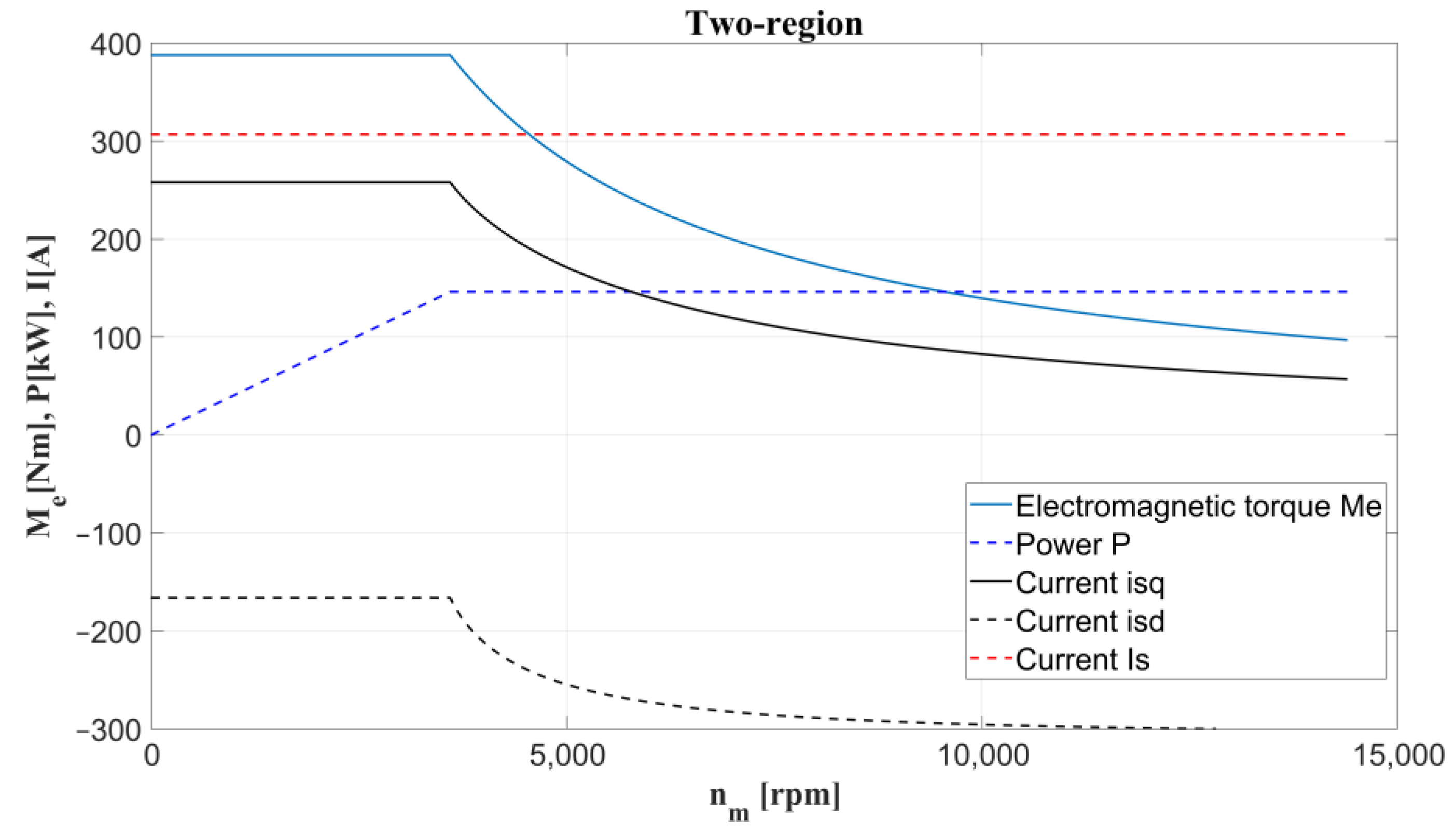
The static characteristics presented in Figure 2 were calculated for the rated data of the motor with 146.2 kW of power (Table 1), which could be used in the main drive of a vehicle.
The curves presented in the figure were calculated for operation with constant torque () and constant power (), as discussed in [1,2,3,4]. In the presented visualization, the current limit was not exceeded, according to Formula (10), and the electromagnetic torque was determined from relation (9). It can be seen from the obtained characteristics that the first control region, for constant torque, ended when the motor reached its rated speed, i.e., 3600 rpm. Then, the flux-weakening operation began (constant power operation).
3.2. Operating Characteristics of the Traction Motor with Interior Magnets
This chapter provides static characteristics for the IPMSM with similar parameters to those shown in Table 1. The difference is the inclusion of stator inductance asymmetry, which is related to the design of rotors with interior magnets. Here, a reluctance torque is generated in the motor in addition to the synchronous torque. In fact, the value of the electromagnetic torque is determined from the same relation as that used for the SMPMSM (9). This is because the distribution of the linked stator fluxes is taken into account (Equations (7) and (8)). The axes have an uneven distribution of inductance ; thus, the distribution was assumed.
The system of the equations consists of two relationships:
Figure 3 presents the correct determination of the characteristics of two-region motor control with the interior magnets. The current values in the first region differed from the SMPMSM values. For constant torque control, the current must be different from zero; in this case, it should be A, and the current should be different from the value so that both conditions are met at the same time. This means that the generation of the reluctance and the synchronous torque is produced by the motor.
The magnetic flux of the stator was determined using the following formula:
A comparison of the flux characteristics of the two motors is shown in the Figure 4.
The calculations were performed in Matlab using its basic functions and the built-in fsolve function, which is used to solve non-linear equations with many variables (12).
The results of the calculations based on Equations (7), (8), (11) and (12), which are shown in Figure 4, showed what effect the rotor structure had on the motor stator flux. It can be seen that the flux was increased in IPMSMs; however, this involves a more complicated design, which obviously must be more expensive.
The results presented in Figure 2, Figure 3 and Figure 4 were realized based on an algorithm for determining of the static characteristics of the two-region motor control of the PMSM, which is shown in Figure 5.
The presented algorithm determines the current values separately for the constant torque operating zone and for the flux weakening region, which allows for higher than rated angular velocities.
3.3. Designing the Motor Torque Control System with the PMSM for EV Application
The torque and current controllers of the stator in the axis were properly selected to design the control system. The controller parameters in simplified motor models [18,20] were determined, and simulations were also carried out for the complete model in the frame.
Figure 6 shows a schematic diagram of the permanent magnet synchronous motor (PMSM) control system for an EV. The system uses torque and current controllers. There are prefilters in the input of each controller for the smoothing of waveforms.
The motor torque control system, which depends on angular speed, was implemented in the reference system; thus, the Clarke and Park transformations were neglected.
The new symbols (electromagnetic time constants) are shown in Figure 6: . The blue blocks are PI controllers, the green blocks are prefilters, and the red block is the command (reference) signal generator, which produces the signals shown in Figure 2 and Figure 3.
The load torque is calculated from the road loads [1,18,19,21]: total rolling resistance , aerodynamic drag force , and grade resistance . Thus, the total road load can be expressed in the following form:
where , , , is the rolling coefficient ( for a concrete road), is the mass of the car and passengers, is the air density, is the drag coefficient, is the frontal area of the car, is the car speed, is the speed of wind, and is the slope.
Hence, if the gear ratio is , is the wheel diameter, and is Coulomb friction in the gear, then the load torque is equal to:
The total moment of inertia is the sum of three energy storages calculated to the motor side (motor shaft) [16]:
where is the PMSM moment of inertia and is the moment of inertia of the wheels (rims and tires), brake discs, and shafts, which are reduced to the motor shaft.
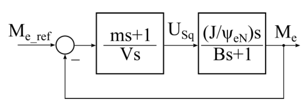
To determine the parameters of the torque controller, the PMSM was linearized and set to a simplified separately excited DC motor. Figure 7 shows the electromagnetic torque control system for a simplified mathematical model of the motor. Mathematical models of motors supplied from voltage sources are discussed in detail in [20], and these models can be approximated by inertial elements. Then, the process of selecting controller settings is simplified, and the controller should be able to overcome the model errors—as shown in the simulations.
The new symbols in Figure 7 are the electromechanical time constant and the flux for the rated current in the axis, where , .
The torque controller is a PI type, where its gain is and the integrating time is . The controller parameters can be expressed in the following form:
A PI controller is also used in the current circuit in the axis. The system used for determining the controller parameters is shown in Figure 8.
The controller parameters in the PMSM take the following form:
The controller (Figure 8) is very aggressive, i.e., it achieves steady state quickly. It may happen that the value of is negative, in which case should be decreased, e.g., , and the results will be similar to those shown.
To simulate the motor with internal magnets, the initial value of the current had to be constant in the first region and different from zero . Using the program for determining static characteristics, we were able to calculate the value that was used for the simulation. The currents in the first region were:
3.4. Simulation Results of Fisker Karma Vehicle with 2 × 146 kW Motors
The original Fisker Karma (Table 2) is a hybrid vehicle equipped with two electric motors, an internal combustion engine, and solar batteries [22,23].
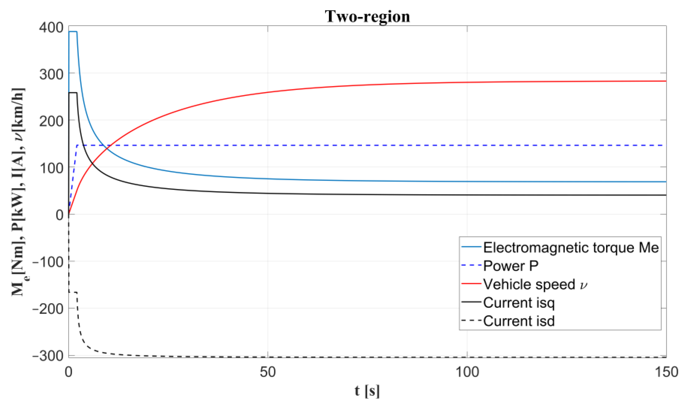
In this study, two IPMSMs with the parameters listed in Table 1 were considered for use in a vehicle powertrain. The parallel operation of the motors was assumed in the design; thus, the mechanical characteristics from Figure 3 were considered, where the electromagnetic torque rating was equal to 776 Nm. The controller parameters were adopted from expressions (17) and (18), and the control system (Figure 6) was simulated in the Matlab-Simulink environment. The results are presented in Figure 9, where the vehicle acceleration dynamics are shown; the acceleration signal in Figure 6 (left side of the red block) was set to 1.
In the presented results, the vehicle was assumed to move under a load of 390 kg (five people) and had a theoretical maximum speed of 280 km/h. Moreover, the region of the constant torque operation was very short, and most of the time it was in constant power operation.
The road loads and the traction force for this simulation are presented in Figure 10. The motor torque was transformed into the traction force on the car wheels using the following formula:
The function is the global load force for an EV and can be recalculated to load torque for a PMSM.
3.5. Simulation Results of Fisker Karma Vehicle with 2 × 100 kW Motors
Since it is difficult to perform experimental tests for the case considered in this paper (EV with programmable current controllers), the application of the algorithm to other motors and simulation verifications will be presented. The motor parameters were taken from [16] (Table 3), where the value of the moment of inertia , which was not given in [16], was approximated on the basis of the ratio rules (high-speed vs. medium-speed motors and power).
The characteristics resulting from (10) and (12) are shown in Figure 11 and are similar to those shown in Figure 3. The differences are due to the different power, the different rated angular velocity, and, of course, the parameters of the machine itself.
By using the algorithm for determining the static characteristics (Figure 5), the values of the currents for the first zone were determined. The constant values of the currents in the and axes for the first zone were used in the simulation in order to calculate the dynamic characteristics. The values of these currents were:
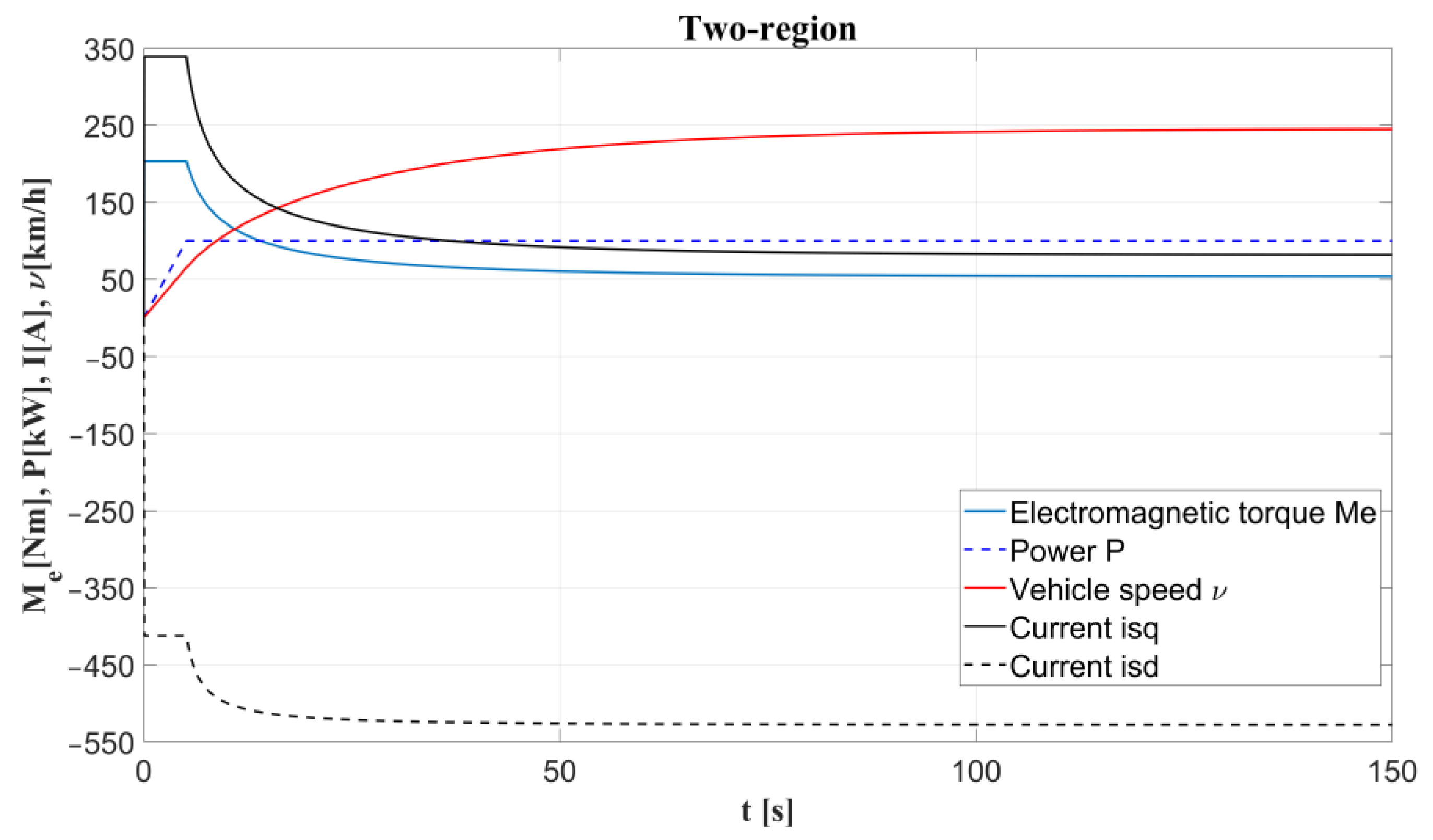
The simulation results for the Fisker Karma with two 100 kW PMSMs are shown in Figure 12 and Figure 13. Obviously, the performance was worse than that of the 146 kW motors; however, the waveform presentation was similar.
In the presented results, the vehicle was assumed to move under a load of 390 kg (five people) and had a theoretical maximum speed equal to 245 km/h.
The simulations in Figure 10 and Figure 13 show how the vehicle’s resistance to motion, or load torque, will change for the electric motor. When the forces balance, the vehicle no longer accelerates.
In the simulation results presented in Figure 9, Figure 10, Figure 11, Figure 12 and Figure 13, the static characteristics from Figure 3 and Figure 11 were used as the reference signals ( and ) for the current controllers (Figure 6). Figure 9 and Figure 12 show the acceleration of the EV when the set electromagnetic torque was at its maximum; this was equivalent to maximum accelerator pedal depression by the driver, which here was considered as the speed controller. The motion of the vehicle was presented by the speed waveform. The resistance of motion is shown in Figure 10 and Figure 13, which are plotted against the traction force waveform . From the waveforms, it can be seen that the operation of the PMSM in the region of constant torque lasted for about 6 or 9 s; then, the motion resistances were small and increased as the EV speed increased. Therefore, the acceleration of the vehicle was accompanied by an almost linear increase in speed. After that, the acceleration of the vehicle began to decrease; this was the influence of both the operation of the motors at constant power and the increase in the load, which is related to vehicle speed according to Equations (14) and (15). The presented waveforms allowed us to determine the performance of the vehicle, such as its maximum speed and acceleration to 100 kmh or 60 mph.
The obtained results confirmed the correct design of the EV drive control system, part of which was the reference signal generator (the realization of static characteristics depending on the angular speed of the motor). The considered problem was confirmed by two computational simulation solutions, where the dynamics of vehicle motion were taken into account.
In the obtained simulation results, a constant torque and constant power algorithm similar to that described in [4,5,6,7,8,9,10,11,12] was used; thus, the presented mechanical characteristics agree with the literature. MTPV (maximum torque per voltage) and MTPA (maximum torque per ampere) algorithms were not used here because they introduce torque oscillation, which is disadvantageous for passengers during car acceleration. A smooth motor start up to a desired speed was presented only in papers [6,11]—as well as in this paper. In the others, it was a three-stage operation, i.e., starting up to nominal speed, operation at a constant speed, and field weakening. This approach is associated with oscillation during the transition from constant torque to constant power operation—this is unacceptable in EV drives. The method presented in this paper can overcome these problems.
Comparing the results presented here with the literature where “EV” is in the title (EV is now a popular phrase, but not always appropriate to the topic of the article) is difficult; they all have experimental results, but many do not relate to the specifics of the EV powertrain—usually they are electric drive control systems to which an EV has been added. The basis of the operation of the transmission is flux weakening, and the systems presented in [13,14,24] work for constant torque; that is, they need a gearbox, which is unnecessary in an EV. Some have oscillations in electromagnetic torque, and then the question must be asked: how will the passenger react to such driving conditions? Sliding mode control offers great possibilities; however, in [15], no uniform motor starting is presented, only three-stage continuous problems with a smooth transition from constant torque operation to constant power operation. In addition, in [16], which focused on EVs, only the flux-weakening operation is presented, with no motor angular velocity run. In this case, it is not clear how one should refer to it.
In summary, the results presented here provide an estimate of EV performance (as in publications [18,19]), only in Figure 9 and Figure 12, the set speeds (e.g., 100 kmh) or distances (e.g., 1/4 mile) need to be labeled. Then, we can see how the electric motor and EV dynamics combine. For the example in Section 3.5, an illustration of vehicle performance is shown in Figure 14.
A speed waveform (red line) is included in the figure from which the time for the EV to reach 100 kmh can be read (first time marked with the red dashed line). The figure has been completed with the distance traveled by the vehicle and the time per 1/4 mile (second time marked with the green dashed line) can be determined from the green line. Thus, from the results obtained, the performance of the vehicle can be easily estimated. An acceleration of 8.75 s to 100 kmh and a time of 16.8 s per 1/4 mile were obtained. Changing the drive motors will change the performance of the vehicle, which can be estimated like this.
3.6. Driving Cycles for EV
This subsection contains two simulation experiments with the designed powertrain for an example vehicle, i.e., a Fisker Karma with two 146 kW motors. In the first experiment, the driving cycle considered the slope of the road surface, while the second used the previously mentioned international WLTP driving cycle, which determines the energy consumption for light vehicles within 0.5 h.
The first driving cycle considered a 10% slope at a constant speed of 50 kmh. In automotive engineering, a slope of 45° is taken as 100%; thus, in the case under consideration, it was an angle of 4.5°. This means that the gravitational force must be considered, where , which is almost eight times greater than the rolling resistance ! This will obviously affect the power consumption.
Figure 15 shows the driving cycle with the following slopes: 0%, 10% (up), 0%, −10% (down), and 0%. The different stages are separated by dashed lines. In this study, the whole vehicle was analyzed; thus, the power consumption is for two motors.
It took 2 s to obtain a speed of 50 kmh, then it was assumed to drive on a 0% slope; in 5 s, the slope gently changed until it reached 10%; in 10 s, the terrain again gently returned to 0%; in 15 s, the terrain started to decrease (−10%); and from 20 s, the terrain was 0%.
Most interesting is the red dashed line (energy consumption); here, we can see how much energy is used for going uphill and how much can be recovered when going downhill by recharging the batteries.
The bottom graph shows how the drag forces changed with such a driving cycle; one can see the significant effect of gravity when changing the slope and how big it was—this also increases the combustion in classic combustion vehicles.
The second driving cycle analyzed in this study was the WLTP, which was introduced in 2017 and is one of the tests most commonly used by automakers.
Professional driving cycles are standardized driving patterns created primarily for vehicle engine performance and powertrain testing. These cycles are represented as speed versus time diagrams. The simulation results are shown in Figure 16 and Figure 17.
The normalized driving cycle was converted to the first subplot, which was supplemented with the distance traveled (less than 24 km). This was the reference for the simulation, and from this the waveform of the motor torque and the power taken from and given to the batteries were obtained (subplots 2 and 3).
When the power on the plot is less than 0 W, it can be recovered and recharge the batteries. For this reason, the waveform of battery energy consumption shown in Figure 17 is important.
The sections slow, average, fast, and very fast, are marked with a black dashed line as in Figure 16. In the energy waveform, one can see the changes in the increase and decrease, which correspond to power (positive and negative). Power in turn depends on the motor torque, i.e., positive torque corresponds to motor work and negative torque to generator (recovery) work.
In summary, the analyzed vehicle will consume about 4.2 kWh in the WLTP cycle and will travel about 24 km. This means that in order to travel 100 km, a battery capacity of at least 17.5 kWh would be needed. Thus, for a vehicle with an average range of 400 km, a battery capacity of 70 kWh would be needed. Of course, when travelling at highway speeds, where aerodynamic drag has a significant effect, this range will decrease.
This means that the WLTP driving cycle is dedicated to mixed driving (city and route) and gives average values.
4. Conclusions
The automation of the main component—the PMSM, which converts electrical energy into mechanical energy in the EV—was discussed in the article. The properties of two types of synchronous motors excited by permanent magnets were studied and determined using simulations in the Matlab-Simulink program. An algorithm was developed in order to determine the static characteristics of the two-region motor torque control of any permanent magnet synchronous motor. This helped us to understand and program (reference signal generator) the PMSM control system in Simulink, with which the characteristics of two-region torque control were established.
The vector control of a PMSM was proposed in a rotating coordinate system ( frame) with rotor angular speed, where two controllers, two prefilters, and a reference signal generator were used (the realization of the static characteristics depending on the motor angular speed).
The PI controller parameters were selected in the motor control system and were used to control the electromagnetic torque and the stator current in the axis. The selection of parameters began with the simplest motor model. The advantage of this novel method is that it is a quick and simple way to determine the parameters of the controllers.
Finally, the results of the simulation experiments in the Matlab-Simulink environment confirmed the correctness of the proposed design process. These studies were carried out for the Fisker Karma electric vehicle, where the vehicle acceleration dynamics were analyzed. Additional tests were conducted for road slope changes and for the WLTP driving cycle, which has been the global world standard since 2017. This cycle determines energy consumption, i.e., fuel burn-up or battery discharge, for a given driving speed profile. The results for range were described.
In summary, the following problems were related in this paper: a permanent magnet synchronous motor, its variable load related to the specificity of the road vehicle, the system of and current regulation to realize two-region drive control (for constant torque and for constant power), the system of reference value generation, and the selection of regulator settings. This is what distinguishes this article from other papers, i.e., the solution is dedicated to EVs and is not some kind of control system, which after modification can be used in an EV. The presented results were consistent and allowed us to estimate the performance of the designed vehicle (all the conversion factors were given that allow for the transfer of the entire specifics of the EV to the side of the electric motor), which from now on can be treated as a variable torque drive, where two-region control is necessary.
Author Contributions
Methodology, D.K.; software, D.K. and G.S.; formal analysis, G.S.; resources, G.S.; data curation, D.K.; writing—original draft preparation, D.K. and G.S.; writing—review and editing, D.K. and G.S.; visualization, D.K.; supervision, G.S. All authors have read and agreed to the published version of the manuscript.
Funding
This research received no external funding.
Institutional Review Board Statement
Not applicable.
Informed Consent Statement
Not applicable.
Data Availability Statement
All data used are included in the references.
Conflicts of Interest
The authors declare no conflict of interest.
References
- Nam, K. AC Motor Control and Electrical Vehicle Applications; CRC Press: Boca Raton, FL, USA, 2010. [Google Scholar]
- Krishnan, R. Electric Motor Drives. Modelling, Analysis and Control; Prentice Hall: Upper Saddle River, NJ, USA, 2001. [Google Scholar]
- Krishnan, R. Permanent Magnet Synchronous and Brushless DC Motor Drives; CRC Press: Boca Raton, FL, USA, 2017. [Google Scholar]
- Vaclavek, P.; Blaha, P. Interior permanent magnet synchronous machine field weakening control strategy—The analytical solution. In Proceedings of the 2008 SICE Annual Conference, Tokyo, Japan, 20–22 August 2008; pp. 753–757. [Google Scholar] [CrossRef]
- Sepulchre, L.; Fadel, M.; Ptetrzak-David, M. MTPV for continuous flux-weakening strategy control law for IPMSM. In Proceedings of the 2018 International Symposium on Power Electronics, Electrical Drives, Automation and Motion (SPEEDAM), Amalfi, Italy, 20–22 June 2018; pp. 1221–1226. [Google Scholar] [CrossRef]
- Wang, J.; Wu, J.; Gan, C.; Sun, Q. Comparative study of flux-weakening control methods for PMSM drive over wide speed range. In Proceedings of the 2016 19th International Conference on Electrical Machines and Systems (ICEMS), Chiba, Japan, 13–16 November 2016; pp. 1–6. [Google Scholar]
- Lin, P.; Lai, Y. Voltage control of interior permanent magnet synchronous motor drives to extend DC-link voltage utilization for flux weakening operation. In Proceedings of the IECON 2010—36th Annual Conference on IEEE Industrial Electronics Society, Glendale, AZ, USA, 7–10 November 2010; pp. 1689–1694. [Google Scholar] [CrossRef]
- Sheng, Y.; Zhou, W.; Hong, Z.; Yu, S. Field weakening operation control of permanent magnet synchronous motor for railway vehicles based on maximum electromagnetic torque at full speed. In Proceedings of the 29th Chinese Control Conference, Beijing, China, 29–30 July 2010; pp. 1608–1613. [Google Scholar]
- Zhou, K.; Ai, M.; Sun, D.; Jin, N.; Wu, X. Field Weakening Operation Control Strategies of PMSM Based on Feedback Linearization. Energies 2019, 12, 4526. [Google Scholar] [CrossRef] [Green Version]
- Wei, L.; Hui, L.; Chao, W. Study on flux-weakening control based on Single Current Regulator for PMSM. In Proceedings of the 2014 IEEE Conference and Expo Transportation Electrification Asia-Pacific (ITEC Asia-Pacific), Beijing, China, 31 August–3 September 2014; pp. 1–3. [Google Scholar] [CrossRef]
- Morimoto, S.; Sanada, M.; Takeda, Y. Wide-speed operation of interior permanent magnet synchronous motors with high-performance current regulator. IEEE Trans. Ind. Appl. 1994, 30, 920–926. [Google Scholar] [CrossRef]
- Ekanayake, S.; Dutta, R.; Rahman, M.F.; Xiao, D. Deep flux weakening control of a segmented interior permanent magnet synchronous motor with maximum torque per voltage control. In Proceedings of the IECON 2015—41st Annual Conference of the IEEE Industrial Electronics Society, Yokohama, Japan, 9–12 November 2015; pp. 004802–004807. [Google Scholar] [CrossRef]
- Liao, G.; Zhang, W.; Cai, C. Research on a PMSM control strategy for electric vehicles. Adv. Mech. Eng. 2021, 13, 1–14. [Google Scholar] [CrossRef]
- Morales-Caporal, R.; Leal-López, M.E.; Rangel-Magdaleno, J.d.J.; Sandre-Hernández, O.; Cruz-Vega, I. Direct torque control of a PMSM-drive for electric vehicle applications. In Proceedings of the 2018 International Conference on Electronics, Communications and Computers (CONIELECOMP), Cholula, Mexico, 21–23 February 2018; pp. 232–237. [Google Scholar] [CrossRef]
- Akhil, R.S.; Mini, V.P.; Mayadevi, N.; Harikumar, R. Modified Flux-Weakening Control for Electric Vehicle with PMSM Drive. IFAC-PapersOnLine 2020, 53, 325–331. [Google Scholar] [CrossRef]
- Wei, H.; Yu, J.; Zhang, Y.; Ai, Q. High-speed control strategy for permanent magnet synchronous machines in electric vehicles drives: Analysis of dynamic torque response and instantaneous current compensation. Energy Rep. 2020, 6, 2324–2335. [Google Scholar] [CrossRef]
- E250 Diameter Frames. Available online: http://www.powertecmotors.com/wp-content/uploads/POWERTEC-PACTORQ-Catalog-e-250-Motor-Info-.pdf (accessed on 29 June 2022).
- Sieklucki, G. An Investigation into the induction motor of Tesla Model S vehicle. In Proceedings of the 2018 International Symposium on Electrical Machines (SME), Andrychów, Poland, 10–13 June 2018; pp. 1–6. [Google Scholar] [CrossRef]
- Sieklucki, G. Optimization of Powertrain in EV. Energies 2021, 14, 725. [Google Scholar] [CrossRef]
- Sieklucki, G. Analysis of the transfer-function models of electric drives with voltage controlled source. Przegląd Elektrotechniczny 2012, 88, 250–255. [Google Scholar]
- Gillespie, T. Fundamentals of Vehicle Dynamics; Society of Automotive Engineers: Warrendale, PA, USA, 1992. [Google Scholar]
- Available online: https://www.auto-brochures.com/makes/Fisker/Fisker_US%20Karma_2012.pdf (accessed on 29 June 2022).
- Available online: http://www.autozine.org/Archive/Fisker/old/Karma.html (accessed on 29 June 2022).
- Sharma, T.; Bhattacharva, A. Sensorless direct torque control of PMSM drive for EV application. In Proceedings of the 2018 2nd International Conference on Power, Energy and Environment: Towards Smart Technology (ICEPE), Shillong, India, 1–2 June 2018; pp. 1–6. [Google Scholar] [CrossRef]
Figure 1.
Design of PMSM rotors: (a) with surface magnets; (b) rotor with interior magnets, configuration 1; (c) rotor with interior magnets, configuration 2.
Figure 1.
Design of PMSM rotors: (a) with surface magnets; (b) rotor with interior magnets, configuration 1; (c) rotor with interior magnets, configuration 2.

Figure 2.
Ideal characteristics for the two-region control of an SMPMSM.

Figure 3.
Ideal characteristics for the two-region control of an IPMSM .

Figure 4.
Ideal stator flux characteristics for two-zone PMSM control.

Figure 5.
Algorithm for calculation of PMSM.

Figure 6.
Schematic diagram of the PMSM control system in an EV application.

Figure 7.
Schematic diagram of the electromagnetic torque control system of the simplified motor.

Figure 8.
Schematic diagram of the current control system in the axis of the PMSM.

Figure 9.
Fisker Karma performance. Dynamics of the two-region motor torque control.

Figure 10.
Forces acting on vehicle obtained from simulation results, where is the traction force on the car wheels.
Figure 10.
Forces acting on vehicle obtained from simulation results, where is the traction force on the car wheels.

Figure 11.
Ideal characteristics for the two-region control of a IPMSM.

Figure 12.
Performance of the Fisker Karma with two IPMSMs. Dynamics of the two-region motor torque control.
Figure 12.
Performance of the Fisker Karma with two IPMSMs. Dynamics of the two-region motor torque control.

Figure 13.
Forces acting on vehicle obtained from simulation results for IPMSM.

Figure 14.
EV performance estimation for IPMSM.

Figure 15.
Driving cycle up and down for IPMSM in EV.

Figure 16.
WLTP driving cycle for IPMSM in EV.

Figure 17.
WLTP driving cycle energy consumption.


Table 1.
List of parameters for PMSM with surface magnets.
| Rated power | 146.2 kW |
| Rated electromagnetic torque | 388 Nm |
| Rated rotational speed | 3600 rpm |
| Rated voltage | 640 V |
| Rated current | 217 A |
| Moment of inertia | 0.199 kgm2 |
| Stator resistance | 0.5 Ω |
| Stator inductance | 0.48 mH |
| Number of pole pairs | 4 |
Table 2.
Fisker Karma vehicle parameters list.
| Vehicle mass | 2540 kg |
| Aerodynamic drag coefficient | 0.313 |
| Gear ratio | 6.254 |
| Tires 255/35R22 (wheel diameter) | 0.7373 m |
| Frontal area of the vehicle | 2.47 m2 |
Table 3.
List of parameters for PMSM with surface magnets.
| Rated power | |
| Rated electromagnetic torque | |
| Rated rotational speed | |
| Rated voltage | |
| Rated current | |
| Moment of inertia | |
| Stator resistance | |
| d-axis inductance | |
| q-axis inductance | |
| Number of pole pairs |
Publisher’s Note: MDPI stays neutral with regard to jurisdictional claims in published maps and institutional affiliations. |
© 2022 by the authors. Licensee MDPI, Basel, Switzerland. This article is an open access article distributed under the terms and conditions of the Creative Commons Attribution (CC BY) license (https://creativecommons.org/licenses/by/4.0/).
Share and Cite
MDPI and ACS Style
Sieklucki, G.; Kara, D. Design and Modelling of Energy Conversion with the Two-Region Torque Control of a PMSM in an EV Powertrain. Energies 2022, 15, 4887. https://0-doi-org.brum.beds.ac.uk/10.3390/en15134887
AMA Style
Sieklucki G, Kara D. Design and Modelling of Energy Conversion with the Two-Region Torque Control of a PMSM in an EV Powertrain. Energies. 2022; 15(13):4887. https://0-doi-org.brum.beds.ac.uk/10.3390/en15134887
Chicago/Turabian StyleSieklucki, Grzegorz, and Dawid Kara. 2022. "Design and Modelling of Energy Conversion with the Two-Region Torque Control of a PMSM in an EV Powertrain" Energies 15, no. 13: 4887. https://0-doi-org.brum.beds.ac.uk/10.3390/en15134887
Note that from the first issue of 2016, this journal uses article numbers instead of page numbers. See further details here.