Data Analytics for Admittance Matrix Estimation of Poorly Monitored Distribution Grids

Abstract

Smart grid operations require accurate information on network topology and electrical equipment parameters. This paper proposes estimating such information with data from the smart grid. Assuming that the availability of bus voltage data is restricted to their magnitude, a linear model of the relationship between these data and the parameters of the admittance matrix is derived in a way that does not involve bus voltage angles. A regression optimizer is then proposed to minimize the deviation between data and values estimated by the linear model. Results on the IEEE 33 bus system are presented to illustrate the model accuracy and efficiency when used to estimate parameters of medium-voltage, three-phase balanced grids.

1. Introduction

In recent years, the electrical power system has undergone substantial changes driven by the decarbonization of production and the electrification of consumption. For the changes to be sustainable, the increase in consumption driven by electrification needs to evolve in tandem with the transition towards renewables and with the emergence of flexibility services, whose deployment will have to be widespread in order to be effective. The combination of a higher demand, distributed renewables and flexibility services will challenge existing power grids, especially distribution networks, increasing stress over grid operators to ensure a secure supply and to maintain quality of service [1].

To overcome this challenge, advanced operation and control systems must be in place, requiring an enhanced understanding of network loads, distributed resources and infrastructure characteristics [2]. In this context, it is crucial to have the best information possible about loads and infrastructure characteristics. Many important efforts have been made to improve load forecasting and load modeling in distribution networks [3]. However, network characteristics, in particular power line parameters such as resistances and reactances, remain largely unknown or are known with little accuracy for many distribution networks [4]. On the contrary, high-precision data on bus loads and voltages are being made available by the advanced metering infrastructure (AMI), making it possible in practice to estimate line parameters from the analysis of those high-precision load and voltage data. This paper aims at advancing such data analytics, in this way contributing to overcome the challenge of a sustainable energy transition based on smart grids.

The problem of electrical grid line parameter estimation has been addressed before, relying upon sets of measurements of both active and reactive power injections, P and Q, and the corresponding measurements of both voltage magnitudes and angles, $\left|V\right|$ and $\theta$ [4,5,6,7,8]. However, the proposed algorithms require data on every single variable $(P,Q,|V|,\theta )$ for every single bus of the grid, making their use to estimate distribution grid parameters impractical, as such grids are typically not monitored on the voltage angles, $\theta$. Voltage angles require micro-phasor mesurement units ($\mu$PMU) to be deployed, and these are too expensive to deploy on each and every distribution load bus [9].

Other approaches have been proposed that make use of complex graph theory to overcome the aforementioned problem [4,10,11,12]. These rely upon much more complex implementation procedures, whose results are usually sensitive to the optimization procedure used. One of the most effective methods proposed in the literature to overcome the lack of data on voltage angles is presented in [13]. In their paper, the authors use an extended linear power-flow model (a Jacobian) to express $P,Q$ on $\left|V\right|$ and $\theta$ measurement data, and then remove the dependence on $\theta$ by Gaussian elimination. This method proved to be accurate despite the complexities involved in the Gaussian elimination procedures.

As in previous approaches, the focus of our paper is on parameter estimation for medium voltage (MV) distribution grids, assuming those grids can be modelled as three-phase balanced systems. During parameter estimation, it is assumed that there is prior knowledge on grid topology. The topology estimation is not addressed in this study given that it is usually well-known for MV distribution grids. Specific algorithms for topology estimation can be found as part of the state estimation literature [8,10,11,12,14].

To estimate line parameters in MV distribution grids, our paper presents a simpler yet robust method to deal with the lack of data on voltage angles. It uses an approximation of the inverted Jacobian to express voltage magnitudes $\left|V\right|$ directly on the injection data $P,Q$, this way avoiding the need for Gaussian elimination procedures while providing very accurate results. The paper is organized as follows: In Section 2, the background for the linear approximation of the problem is provided. In Section 3, the methodology to solve the linear problem is proposed. In Section 4, the most important results are summarized and model limitations are analyzed. Finally, in Section 5, the main conclusions are presented.

2. Background

2.1. Exact Power-Flow Equations

Power flow equations are usually expressed in a way that relates nodal active and reactive power injections with the grid voltage magnitudes and corresponding angles. For a given electrical grid, the relationship involves the admittance matrix parameters, whose values derive from the the electrical line parameters connecting the grid buses. Classical power flow equations (two per bus i) are expressed for such parameters as the following:

$$P_i=\sum _{j=1}^n{G}_{ij}|V_i||V_j|cos\left({\theta }_{ij}\right)+\sum _{j=1}^n{B}_{ij}|V_i||V_j|sin\left({\theta }_{ij}\right)i=1,2\dots ,n$$

(1)

$$Q_i=-\sum _{j=1}^n{B}_{ij}|V_i||V_j|cos\left({\theta }_{ij}\right)+\sum _{j=1}^n{G}_{ij}|V_i||V_j|sin\left({\theta }_{ij}\right)i=1,2\dots ,n$$

(2)

where $P_i$, $Q_i$ and $|V_i|$ represent the active and reactive power injection, and voltage magnitude at each node i, respectively, and $B_{ij}$ and $G_{ij}$ represent the corresponding nodal conductance and susceptance matrix parameters for the entries i and j. ${\theta }_{ij}$ represents the difference ${\theta }_i-{\theta }_j$ between the voltage angles in bus i and bus j, respectively.

Power flow equations are non-linear with regard to the voltages, both in terms of their magnitudes and angles. However, these equations can be approximated by linear models assuming certain grid characteristics and a limited range of operation conditions. Linear approaches involve an approximation that provides a solution to the power flow analysis problem that does not require numerical methods to be solved. Additionally, and very importantly in the context of this paper, linear approaches can be easily inverted and used for estimation. Several linear models have been presented in the literature [15]. However, most of these account for the active power component only, not considering the reactive component or requiring full measurements of the voltage phasor when considering it, P, Q, $\left|V\right|$ and $\theta$.

2.2. Extended DC Power Flow Approximation

The power flow Equations (1) and (2) can be combined into a single equation, as follows:

$$S_i^{\ast }=V_i^{\ast }\sum _{j=1}^n{y}_{ij}(V_i-V_j),i=1,\cdots ,n$$

(3)

where $S_i^{\ast }=P_i-j{Q}_i$, $V_i$ is the complex voltage at node i and $y_{ij}$ is the corresponding complex element of the nodal admittance matrix Y. In matrix form for all nodes, the equation can be expressed as a vector-valued Ohm law by:

$$I=YV$$

(4)

where I and V are column vectors with nodal current injections and complex voltages, respectively. Making the usual assumptions for linear power flows [16,17], the inversion of (4) can be expressed as:

$$V\approx Z\left[\begin{array}{c}{S}^{\ast }/\left|V\right|\end{array}\right]$$

(5)

where $Z=Y^{-1}$ is the nodal impedance matrix. If one decomposes (5) into its real and imaginary parts, the following difference equation holds:

$$\left[\begin{array}{c}\Delta \theta \\ \Delta \left|V\right|\end{array}\right]\approx \left[\begin{array}{cc}X& -R\\ R& X\end{array}\right]\left[\begin{array}{c}\Delta P/\left|V\right|\\ \Delta Q/\left|V\right|\end{array}\right]$$

(6)

where $R=real\left\{Y\right\}$, $X=imag\left\{Y\right\}$, and $\Delta P$ and $\Delta Q$ are the vector of the nodal active and reactive power injection changes, respectively. To account for the monitoring limitations of distribution grids, namely the lack of measurements on the argument of nodal voltages, this paper makes use of the voltage magnitude equations alone:

$$\left[\begin{array}{c}\Delta \left|V\right|\end{array}\right]\approx \left[\begin{array}{cc}R& X\end{array}\right]\left[\begin{array}{c}\Delta P/\left|V\right|\\ \Delta Q/\left|V\right|\end{array}\right].$$

(7)

3. Solution Methodology

3.1. Regression Model

The linear relationship of (7) can be rewritten in a different manner, providing a linear relationship between bus voltage magnitudes $\Delta \left|V\right|$ and the R and X sub-matrices, as presented below.

$$\left[\begin{array}{c}\Delta |V_{0i}|\end{array}\right]\approx \left[\begin{array}{cc}\Delta P/\left|V\right|& \Delta Q/\left|V\right|\end{array}\right]\left[\begin{array}{c}R\\ X\end{array}\right]$$

(8)

where $|V_{0i}|$ is the voltage drop between a reference node 0 and the remaining nodes i, and $\Delta P/\left|V\right|$ and $\Delta Q/\left|V\right|$ account for the active and reactive power injection at each node divided by the corresponding voltage magnitude, respectively.

The existence of linearly dependent vectors makes the inversion of the full measurement matrix $[\Delta P/|V|\Delta Q/|V\left|\right]$ infeasible, this way compromising the estimation of the admittance matrix. The reconstruction of only a part of the admittance matrix is sometimes possible [4,12]. A well-known dependency is the one involving the reference bus, whose equation needs to be removed in order to obtain a set of linearly independent power flow equations [13]. We opted for writing the equations as difference equations on the voltage drops $|V_{0i}|$ between every node i and the reference node 0 (which we can compute directly from data), this way avoiding the need to remove and add equations to the power flow model in order to be able to invert it. The following algorithm summarizes the three steps necessary to build the new system (8) in a way that preserves the relationships expressed in (7).

3.2. Proposed Solution

The transformation matrix in (8) must have more equations than unknowns, i.e., more rows than columns. This is easy to accomplish since large sets of data are being collected regularly from AMI and other meters deployed in smart grids. If the assumption holds, a linear regression algorithm can be used to estimate the parameters of both R and X [18]. The choice of linear regression has the purpose of preserving interpretability to the detriment of predictive potential. More complex algorithms could perhaps perform better, but usually embody some kind of impenetrable black-box reasoning while requiring sensible training for parameterization—something that often turns out to be impractical for real-world applications. We use the ordinary least-squares (OLS) algorithm to regress over the data. The following expression provides the well-known OLS regression formula:

$$\begin{array}{c}\hfill \widehat{\beta }={\left(A^{T}A\right)}^{-1}{A}^{T}y\end{array}$$

(9)

where:

$$A=\left[\begin{array}{cc}\Delta P/\left|V\right|& \Delta Q/\left|V\right|\end{array}\right]$$

(10)

$$y=\left[\begin{array}{c}\Delta |V_{bi}|\end{array}\right]$$

(11)

$$\widehat{\beta }=\left[\begin{array}{c}R\\ X\end{array}\right].$$

(12)

As explained in Algorithm 1, matrix A is constructed with information on $\Delta P/\left|V\right|$ and $\Delta Q/\left|V\right|$, measurements collected and available from the AMI. Vector y contains information about voltage drops that can be easily computed as diferences between the reference node 0 and the remaining nodes of the grid. The vector $\widehat{\beta }$ corresponds to the R-X parameters to be discovered.

Algorithm 1 Construction of the matrices of (8).

Step 1: Compute the Voltage Drop Vector

${\left.\left[\Delta \left|V_{0i}\right|\right]={\left[\begin{array}{c}\Delta \left|V_{01}\right|\\ \Delta \left|V_{02}\right|\\ ⋮\\ \Delta \left|V_{0i}\right|\end{array}\right]}_1^{\top }{\left[\begin{array}{c}\Delta \left|V_{01}\right|{}^{\top }\\ \Delta \left|V_{02}\right|\\ ⋮\\ \Delta \left|V_{0i}\right|\end{array}\right]}_2^{\top }\dots {\left[\begin{array}{c}\Delta \left|V_{01}\right|\\ \Delta \left|V_{02}\right|\\ ⋮\\ \Delta \left|V_{0i}\right|\end{array}\right]}_t^{\top }\right]}^{\top }$

where:

(1) $i=1,2,\dots ,N_{bus}-1$;

(2) $t=1,2,\dots ,\mathrm{number}\mathrm{of}\mathrm{periods}$;

Step 2: Define the R-X Vector

(1) R = ${\left[\begin{array}{ccccccccccc}{R}_{11}& \cdots & R_{1i}& R_{22}& \cdots & R_{2i}& R_{33}& \cdots & R_{3i}& \cdots & R_{ii}\end{array}\right]}^{\top }$

(2) X = ${\left[\begin{array}{ccccccccccc}{X}_{11}& \cdots & X_{1i}& X_{22}& \cdots & X_{2i}& X_{33}& \cdots & X_{3i}& \cdots & X_{ii}\end{array}\right]}^{\top }$

where: $i=1,2,\dots ,N_{bus}-1$;

Step 3: Compute the Measurements Matrix

$\left[\begin{array}{cc}\Delta P/\left|V\right|& \Delta Q/\left|V\right|\end{array}\right]$ = $\left[\begin{array}{cc}{\left[\Delta P_i/\left|V_i\right|\right]}_1& {\left[\Delta Q_i/\left|V_i\right|\right]}_1\\ {\left[\Delta P_i/\left|V_i\right|\right]}_2& {\left[\Delta Q_i/\left|V_i\right|\right]}_2\\ ⋮& ⋮\\ {\left[\Delta P_i/\left|V_i\right|\right]}_t& {\left[\Delta Q_i/\left|V_i\right|\right]}_t\end{array}\right]$

where:

(1) $i=1,2,\dots ,N_{bus}-1$;

(2) Element’s position on sub-matrices $[\Delta P_i/|V_i{\left|\right]}_t$ and $[\Delta Q_i/|V_i{\left|\right]}_t$ must be coherent with

the R-X vector defined in Step 2, maintaining the same linear structure of (7).

Since the majority of the power flow algorithms and corresponding equations are expressed in the admittance matrix elements (G and B), we will construct the admittance matrix from the information estimated for its inverse, as provided by R and X, and compute errors for the estimated admittance parameters ($\widehat{G}$ and $\widehat{B}$) in order to compare our method with others.

3.3. Feeder Laterals and Non-Metered Buses

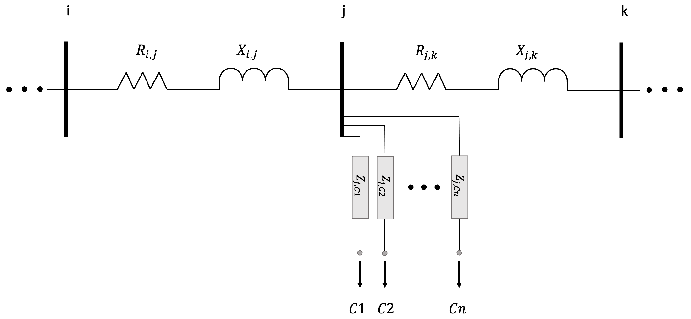
Feeder laterals are derivations from the main feeder used to feed one or multiple consumers, as schematically represented in Figure 1. The feeder derivation nodes (j in the figure) are usually zero-injection nodes for which there are no voltage data available.

The standard approach for feeder laterals is to consider the voltage magnitudes found at the consumer level as close to the magnitudes of the voltage at the feeder derivation node ($|V_j|$ in the figure), since the lateral impedances are usually negligible. In such cases, the proposed method (8) can be applied directly.

For the cases where lateral impedances are not negligible, the voltage magnitudes of feeder derivation nodes may be estimated. In this case, the method needs to be carried out in two steps, as follows:

First, by considering each feeder derivation node and the corresponding consumers as grid subsystems, one may apply the proposed linear regression approach to estimate the feeder lateral impedances. Since the voltage magnitude of the derivation node is unknown, differences between consumer voltage magnitudes are expressed on the lateral impedances alone, as presented in the following linear system:

$$\left[\begin{array}{c}\Delta |V_{Cl,Cm}|\end{array}\right]\approx \left[\begin{array}{cccc}\Delta P_{Cm}/\left|V_{Cm}\right|& \Delta Q_{Cm}/\left|V_{Cm}\right|& -\Delta P_{Cl}/\left|V_{Cl}\right|& -\Delta Q_{Cl}/\left|V_{Cl}\right|\end{array}\right]\left[\begin{array}{c}{R}_{j,Cm}\\ X_{j,Cm}\\ R_{j,Cl}\\ X_{j,Cl}\end{array}\right]$$

(13)

where $m\ne l$, $m=1,\cdots ,n$ and both $Cm$ and $Cl$ represent lateral feeder consumers, as presented in Figure 1.

Second, with the information on the voltage magnitude and consumption at the consumer nodes, and the estimate of the line parameters of the feeder laterals, one may finally estimate the feeder derivation node voltage magnitude using Ohm’s Law. Once all feeder derivation node voltage magnitudes are estimated, it is then possible to apply Algorithm 1 to estimate all the grid main feeder impedances.

4. Data and Results

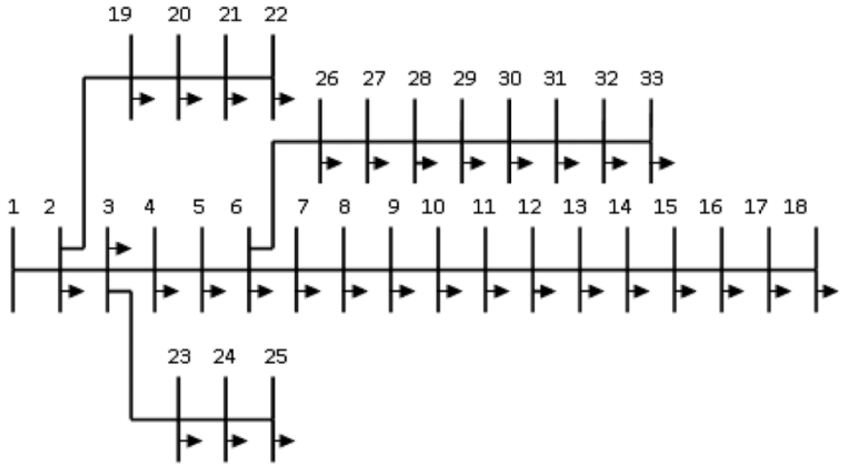
The distribution network used in this study is the IEEE 33 bus system, with the same characteristics and loads as the base model published in [19], but assuming all load buses are three-phase balanced. This three-phase balanced version of the IEEE 33 bus system is a typical distribution system that has been used several times for many different analysis purposes, including the purpose of illustrating data analytics approaches for line-parameter estimation [12,13]. The system is schematically represented in Figure 2.

4.1. Data Set Generation

The data set was synthetically obtained through simulation, in order to make a fair comparison between the present approach and the other models proposed in the literature. The operation of the distribution system was simulated during 300 time intervals by changing 300 different times the initial conditions defined in [19]. Each and every network load was changed independently, sampling its value from a uniform probability distribution function whose range was set to be $\pm 10\%$ of the loads’ original value. The active and reactive load components, P and Q, were also sampled independently in order to vary loads’ power factor in time. With the procedure described, we obtained a coherent set of measurement data on $\left|V\right|$, P and Q, assuming negligible measurement errors over the 300 time periods.

4.2. Results

In this section, the proposed algorithm is evaluated, with a detailed analysis of the errors, and the model limitations are exploited. Errors were quantified using the weighted absolute percentage error (WAPE) metric, defined below, which measures the overall deviation of the estimated values w.r.t. the exact values used in the simulation. The error metric formula is given by:

$${\mathrm{WAPE}}_G=\frac{{\sum }_{i,j=1}^n|G_{ij}-{\widehat{G}}_{ij}|}{{\sum }_{i,j=1}^n\left|G_{ij}\right|},{\mathrm{WAPE}}_B=\frac{{\sum }_{i,j=1}^n|B_{ij}-{\widehat{B}}_{ij}|}{{\sum }_{i,j=1}^n\left|B_{ij}\right|}$$

(14)

where ($G_{ij},B_{ij}$) and (${\widehat{G}}_{ij},{\widehat{B}}_{ij}$) correspond to the exact and the estimated values of both the B and G parameters, respectively.

Under the high loading conditions set for the IEEE 33 bus system in [19], the proposed algorithm can estimate the full admittance matrix with errors of about 3% for either the B or G parameters. The accuracy of the proposed approach is comparable to those proposed in the literature [12,13].

By performing an error sensitivity analysis w.r.t. the total active losses in the system, it is possible to observe that the accuracy of the proposed method is sensitive to losses. Under the above-mentioned load conditions, the system total power losses are about 5–6%, which can be considered a relatively high loss value. If the collected data correspond to periods where total active power losses are close to 1%, then the error obtained for B and G would drastically decrease to values of around 0.4%, which can be considered extremely precise.

The transformation matrix in (8) tends to be very sparse and have a high condition number, which poses a risk of having numerical issues in its inversion. It is therefore important to evaluate how the matrix condition number evolves with the size of the electrical grid under analysis. To illustrate the effect of size on the condition number, the IEEE 33 bus system schematically represented in Figure 2 was decomposed into several sub-grids. These sub-grids were then successively connected while evaluating the resulting matrix condition number. From that starting network of five buses, and in a sequence of five steps in a row, new sub-grids were added in blocks of five buses, computing the matrix condition number in each step. This procedure was applied until the network size achieved a total of 60 buses—a much larger size than the IEEE grid under study.

Figure 3 summarizes the result of the sensitivity analysis carried out, showing how error evolves with total active power losses, and also how the matrix condition number evolves with the number of grid buses.

In Figure 3a, it is clearly noticeable that the estimation error is sensitive to the level of total active power losses. This is due to the fact that the linear relationship of (7) used for regression only involves consumption data per bus, ignoring power losses in the system. As such, when power losses gain a significant scale, e.g., above 2%, the regression model decreases its accuracy and the estimation error increases, e.g., above 1%. However, because large data sets are easily available today, it is usually possible to select load and voltage data concerning periods of low power losses by selecting the data collected at off-peak times.

In Figure 3b, it is shown that the matrix condition number rises quickly above 30, suggesting severe multicollinearity of the transformation matrix for networks above 10 buses. Multicollinearity may lead to ill-conditioned problems, causing the solution to be numerically unstable [20]. Yet, for the IEEE 33 bus system under analysis, even with a high condition number, a good solution can be obtained. However, no guarantees can be provided for other systems or systems of a larger scale. One simple yet effective way to solve this problem is to decompose the electrical grid into sub-grids, providing some scale reduction, and therefore reducing the condition number. A possible division is schematically exemplified below, for the IEEE 33 system of Figure 2.

Since the algorithm is based on voltage drops between a reference node (generally designated as 0) and a given node i, only the downstream consumption with respect to each reference node impacts $\Delta |V_{0i}|$. As such, if one takes buses 2, 3 and 6 as reference nodes, it is possible to independently reconstruct the admittance matrices for each of the sub-grids (a), (b) and (c), as represented in Figure 4. For the remaining sub-grid (d), and following the same reasoning, sub-grids (a), (b) and (c) are represented by meta-nodes A, B and C, whose loads are set to be the aggregate consumption of such sub-grids. With this simple approach to decomposition, it is possible to reduce the size of the transformation matrices and consequently their condition numbers, which can be useful to estimate line parameters of large-scale distribution networks.

5. Conclusions and Future Work

This paper proposes an admittance matrix estimation approach for MV distribution networks whose monitoring infrastructure only provides measurements of bus voltages magnitudes and active and reactive power magnitudes. The proposed approach relies on the linear regression method to estimate the grid admittances, a simpler yet competitive approach w.r.t. the state-of-the-art methods that make use of complex graph theory and optimization algorithms.

Results are provided to illustrate the accuracy and sensitivity to the level of power losses and network scale. For the relatively high power losses case of the IEEE 33 bus system, the algorithm presents an average estimation error of about 3%. Yet, when estimation is based on data obtained at time periods of lower losses, the algorithm presents lower average estimation errors. Future work will focus on extending the approach to address LV unbalanced load situations and on improving the algorithm performance w.r.t. grid losses.

References

- Ilić, M.D.; Carvalho, P.M. From hierarchical control to flexible interactive electricity services: A path to decarbonisation. Electr. Power Syst. Res. 2022, 212, 108554. [Google Scholar] [CrossRef]
- Ardakanian, O.; Keshav, S.; Rosenberg, C. Integration of Renewable Generation and Elastic Loads into Distribution Grids; Springer: Berlin/Heidelberg, Germany, 2016. [Google Scholar]
- Machado, J.A.C.; Carvalho, P.M.S.; Ferreira, L.A.F.M. Building Stochastic Non-Stationary Daily Load/Generation Profiles for Distribution Planning Studies. IEEE Trans. Power Syst. 2018, 33, 911–920. [Google Scholar] [CrossRef]
- Yuan, Y.; Low, S.H.; Ardakanian, O.; Tomlin, C.J. Inverse power flow problem. IEEE Trans. Control. Netw. Syst. 2022; early access. [Google Scholar] [CrossRef]
- Ritzmann, D.; Wright, P.S.; Holderbaum, W.; Potter, B. A method for accurate transmission line impedance parameter estimation. IEEE Trans. Instrum. Meas. 2016, 65, 2204–2213. [Google Scholar] [CrossRef]
- Mousavi-Seyedi, S.S.; Aminifar, F.; Afsharnia, S. Parameter estimation of multiterminal transmission lines using joint PMU and SCADA data. IEEE Trans. Power Deliv. 2014, 30, 1077–1085. [Google Scholar] [CrossRef]
- Sivanagaraju, G.; Chakrabarti, S.; Srivastava, S.C. Uncertainty in transmission line parameters: Estimation and impact on line current differential protection. IEEE Trans. Instrum. Meas. 2013, 63, 1496–1504. [Google Scholar] [CrossRef]
- Farajollahi, M.; Shahsavari, A.; Mohsenian-Rad, H. Topology identification in distribution systems using line current sensors: An MILP approach. IEEE Trans. Smart Grid 2019, 11, 1159–1170. [Google Scholar] [CrossRef]
- Wu, Z.; Du, X.; Gu, W.; Ling, P.; Liu, J.; Fang, C. Optimal Micro-PMU Placement Using Mutual Information Theory in Distribution Networks. Energies 2018, 11, 1917. [Google Scholar] [CrossRef] [Green Version]
- Yu, J.; Weng, Y.; Rajagopal, R. PaToPaEM: A data-driven parameter and topology joint estimation framework for time-varying system in distribution grids. IEEE Trans. Power Syst. 2018, 34, 1682–1692. [Google Scholar] [CrossRef] [Green Version]
- Park, S.; Deka, D.; Chcrtkov, M. Exact topology and parameter estimation in distribution grids with minimal observability. In Proceedings of the 2018 IEEE Power Systems Computation Conference (PSCC), Dublin, Ireland, 11–15 June 2018; pp. 1–6. [Google Scholar]
- Ardakanian, O.; Wong, V.W.; Dobbe, R.; Low, S.H.; von Meier, A.; Tomlin, C.J.; Yuan, Y. On identification of distribution grids. IEEE Trans. Control. Netw. Syst. 2019, 6, 950–960. [Google Scholar] [CrossRef]
- Zhang, J.; Wang, P.; Zhang, N. Distribution network admittance matrix estimation with linear regression. IEEE Trans. Power Syst. 2021, 36, 4896–4899. [Google Scholar] [CrossRef]
- Singh, R.; Manitsas, E.; Pal, B.C.; Strbac, G. A Recursive Bayesian Approach for Identification of Network Configuration Changes in Distribution System State Estimation. IEEE Trans. Power Syst. 2010, 25, 1329–1336. [Google Scholar] [CrossRef]
- Stott, B.; Jardim, J.; Alsaç, O. DC power flow revisited. IEEE Trans. Power Syst. 2009, 24, 1290–1300. [Google Scholar] [CrossRef]
- Guggilam, S.S.; Dall’Anese, E.; Chen, Y.C.; Dhople, S.V.; Giannakis, G.B. Scalable optimization methods for distribution networks with high PV integration. IEEE Trans. Smart Grid 2016, 7, 2061–2070. [Google Scholar] [CrossRef]
- Yang, J.; Zhang, N.; Kang, C.; Xia, Q. A state-independent linear power flow model with accurate estimation of voltage magnitude. IEEE Trans. Power Syst. 2016, 32, 3607–3617. [Google Scholar] [CrossRef]
- Weisberg, S. Applied Linear Regression; John Wiley & Sons: Hoboken, NJ, USA, 2005; Volume 528. [Google Scholar]
- Dolatabadi, S.H.; Ghorbanian, M.; Siano, P.; Hatziargyriou, N.D. An enhanced IEEE 33 bus benchmark test system for distribution system studies. IEEE Trans. Power Syst. 2020, 36, 2565–2572. [Google Scholar] [CrossRef]
- Belsley, D.A.; Kuh, E.; Welsch, R.E. Regression Diagnostics: Identifying Influential Data and Sources of Collinearity; John Wiley & Sons: Hoboken, NJ, USA, 2005. [Google Scholar]
Figure 1.
Feeder lateral example where i and k correspond to standard network load buses and j corresponds to a node to which feeder laterals are connected to supply consumers .
Figure 2.
IEEE 33 bus system used for illustration.
Figure 3.
Sensitivity Analysis: (a) Parameter error evolution with total active power losses. (b) Matrix condition number evolution with the number of network buses.
Figure 4.
Sub-grid topology decomposition. Reference nodes of each sub-grid are circled in red. Sub-grids (a–c) are connected to the grey circles of sub-grid (d) whose reference node is bus 1.
Publisher’s Note: MDPI stays neutral with regard to jurisdictional claims in published maps and institutional affiliations. |
© 2022 by the authors. Licensee MDPI, Basel, Switzerland. This article is an open access article distributed under the terms and conditions of the Creative Commons Attribution (CC BY) license (https://creativecommons.org/licenses/by/4.0/).
Share and Cite
MDPI and ACS Style
Leal, P.C.; Ferreira, D.M.V.P.; Carvalho, P.M.S. Data Analytics for Admittance Matrix Estimation of Poorly Monitored Distribution Grids. Energies 2022, 15, 8961. https://0-doi-org.brum.beds.ac.uk/10.3390/en15238961
AMA Style
Leal PC, Ferreira DMVP, Carvalho PMS. Data Analytics for Admittance Matrix Estimation of Poorly Monitored Distribution Grids. Energies. 2022; 15(23):8961. https://0-doi-org.brum.beds.ac.uk/10.3390/en15238961
Chicago/Turabian StyleLeal, Pedro C., Diogo M. V. P. Ferreira, and Pedro M. S. Carvalho. 2022. "Data Analytics for Admittance Matrix Estimation of Poorly Monitored Distribution Grids" Energies 15, no. 23: 8961. https://0-doi-org.brum.beds.ac.uk/10.3390/en15238961
Note that from the first issue of 2016, this journal uses article numbers instead of page numbers. See further details here.