Genetic-Algorithm-Based Optimization of a 3D Transmitting Coil Design with a Homogeneous Magnetic Field Distribution in a WPT System

Abstract

In magnetically coupled resonant wireless power transfer (MCR-WPT) systems, the nonhomogeneous magnetic field of the transmitting coil can lead to frequency splitting phenomena and lower efficiency. In this paper, a 3D transmitting coil (TX) with a homogeneous magnetic field distribution is proposed. The proposed coil structure consists of two layers with different numbers of turns per layer, i.e., with different current distributions. To achieve a homogeneous magnetic field distribution with a high magnetic field value and a low profile of the 3D coil structure, the optimal layer placement and current distribution were optimized using a genetic algorithm (GA). The prototype of the optimized coil was fabricated, and its magnetic field distribution was measured. The measurement results agreed more than 95% with the simulation results. The measured homogeneous area was at least 12.5% larger than reported in the literature. By using a different current distribution, the profile of the 3D coil structure was successfully reduced by 29% and the average magnetic field value was increased by 25% compared to our previous work.

1. Introduction

A prominent issue in MCR-WPT systems is the degradation of transfer efficiency due to lateral misalignment between the TX coil and the receiving (RX) coil. Usually, the RX coil must be placed at a specific location in the charging plane to achieve high transfer efficiency. However, the MCR-WPT system requires that the position of the RX coil(s) not be precisely specified. The MCR-WPT systems, which require the position of the RX coil to be precisely fixed, are not suitable for the simultaneous charging of multiple, freely movable RX coils. In addition, the wireless charging of implanted medical devices and electric vehicles requires a higher misalignment tolerance, as precise alignment is often difficult to achieve.

Although other parameters also play a role, the degradation of transfer efficiency is most strongly correlated with the decrease in the coupling coefficient k between the TX and the RX coil [1]. To keep k stable, TX coils are required to produce a homogeneous magnetic field intensity distribution in the charging plane [2]. This enables a higher misalignment tolerance. Consequently, stable transfer efficiency and output power are characteristic of such an MCR-WPT system.

Most TX coils designed to produce a homogeneous magnetic field intensity are planar. The hybrid TX coil structure designed in [3] combines a spiral and a concentrated coil to produce a homogeneous magnetic field intensity distribution. The geometry of the planar rectangular spiral coil with blunted corners is optimized to ensure a smooth distribution of the magnetic field in the charging plane [4,5]. A homogeneous magnetic field is achieved by a hybrid TX coil with a reversed current direction between the loops [6]. Based on the current distribution required to produce a defined homogeneous magnetic field distribution, an equivalent TX coil winding distribution with equal current in each winding was applied [7]. In [8], half of the current of the outer windings flows through the inner windings of the TX coil, ensuring a higher misalignment tolerance. Furthermore, in [9], the principle of the current distribution between the windings of the TX coil was presented. As proposed in [10], the square spiral TX coil, with the adjusted position and current of each turn, produces improved homogeneity of the magnetic field in the charging plane. The current distribution between the windings connected in parallel is controlled by a series capacitance added to each winding. The Taichi coil [1] and serpentine coil [11] have also been proposed to improve the misalignment tolerance. Other planar solutions include the square TX coil consisting of one outer and three inner coils [12] and the square TX coil with one outer and one inner coil [13], which requires an optimized RX coil design for optimal transfer efficiency. Although homogeneity was achieved, the planar TX coils were relatively small and transmitted power mainly over short distances (up to 1.5 cm) [2,3,4,5,6,7,8,9,10]. To increase the homogeneous area (part of the charging plane at which a homogeneous magnetic field intensity is produced), an array of TX coils was proposed [7]. However, an additional detection circuit is then required. GA-based optimization of rectangular planar coils has been successfully performed for a large air gap of 10 cm [14]. Nevertheless, the homogeneous area occupied less than 50% of the charging plane.

TX coils are not as critical in terms of planarity compared to RX coils. To achieve high transfer efficiency, RX coils should be flat and parallel with the charging plane. Three-dimensional TX coils are intended for applications where a low TX coil profile is not as important as it is for planar TX coils. The rectangular spatial coil with a height of 14 mm proposed in [15] generates a homogeneous magnetic field intensity in the charging plane. However, due to the large transfer distance, a high supply current is required to transfer a significant amount of power. The spatial TX coil for a WPT system, which creates a homogeneous area, was presented in [16]. However, it was fabricated using printed circuit board technology, which is not suitable for large-scale TX coils.

This paper is a continuation of our research on the development of rectangular coil structures that can produce a homogeneous magnetic field intensity distribution. In previous research, the basic structure of a 3D rectangular coil was proposed and results comparable to the state-of-the-art were obtained (the homogeneous area corresponded to 55% of the charging plane) [17]. In this paper, we were interested in further increasing the homogeneous area and the average magnetic field intensity, but also in reducing the coil profile (height). To achieve this, we used the current distribution approach [9] in coil optimization. In the previous study [17], the homogeneous magnetic field intensity distribution was achieved by optimizing the placement of the coil layers. In this paper, with a different current distribution between the coil layers, an additional dimension was added to the optimization process. The general TX coil design is described in the next section. The following section focuses on the GA optimization of the coil design. Based on the optimization solutions, the GA-optimized coil prototype was fabricated. In the Measurements Section, the simulation and measurement results are compared. Finally, the conclusion summarizes the main results of the optimized coil.

2. General TX Coil Design

In planar MCR-WPT, the RX coil is placed or moved horizontally in the charging plane. Thus, the RX coil is constantly parallel with the TX coil below the charging plane. The magnetic flux captured by the RX coil is then contributed by the vertical magnetic field [2]. From now on, only the vertical component of the magnetic field intensity H_y is considered in the following part of this paper.

The basic outline of the TX coil optimized in this paper is shown in Figure 1. The coil consists of two layers with an identical shape, whose main function is to create a homogeneous magnetic field intensity distribution in the charging plane (gray horizontal surface (xz-plane) in Figure 1). The first coil layer can be distinguished from the second coil layer by its color, black and red, respectively. The length of the coil is denoted by L, while the width of the first coil layer is denoted by W, and the width of the second coil layer is denoted by W₂. The vertical distance between the first and second coil layer along the coil length L is denoted by D₂. The first coil layer is folded to the extent of D, and the second coil layer is also folded to an extent equal to D-D₂. The transfer distance, h, is the vertical distance between the top of the TX coil and the charging plane. The folded TX coil sides originate from the rectangular coil and its magnetic field intensity distribution in the charging plane. Due to the superposition of the magnetic field at the corners of a rectangular coil, the magnetic field intensity distribution in the charging plane over such a coil is nonhomogeneous [17]. Therefore, the shorter sides of the rectangular coil are folded down to eliminate the magnetic field peaks near the corners of the charging plane. Without the second coil layer, there is a saddle-shaped magnetic field intensity distribution across the transverse line (dashed blue line) in Figure 1. Thus, the purpose of the second coil layer is to flatten the shape of the saddle-shaped magnetic field intensity distribution across the transverse line of the charging plane.

3. TX Coil Optimization

In order to enlarge the homogeneous area of the charging plane and achieve a higher average magnetic field intensity within the homogeneous area, an optimization of the design of the TX coil based on a GA was performed. Metaheuristic optimization methods, unlike mathematical optimization methods (programming), allow the specification of arbitrary cost functions (including non-continuous, non-differentiable functions). There is no exact analytical function that relates our specific TX coil geometry and magnetic field intensity. For approximate calculations of the magnetic field intensity, the Biot–Savart law could be applied, but for more realistic results, Ansys Maxwell software was used to calculate magnetic field intensity. In our case, since there was no exact analytical function to define the cost function, the simulation of the magnetic fields was performed. The GA was applied because it is the only type of metaheuristic method available in the Ansys Maxwell Optimetrics tool. A brief description of the GA optimization technique follows, followed by two subsections discussing the detailed implementation of the GA optimization of the coil considered in this paper.

3.1. Genetic Algorithm

The GA is a form of evolutionary algorithm (EA) that mimics the features of natural selection such as selection, crossover, and mutation [18]. The GA is an iterative process that goes through a series of generations. Each generation consists of a number of individuals (parents and offspring) that are selected based on a fitness function (more suitable individuals are preferred—selection operator). Crossover and mutation operators ensure that new individuals are generated in each generation. In elitist selection, the best individuals are selected. Another possibility is roulette selection, in which the fitter an individual is, the higher its probability of survival. Such a random selection of individuals to proceed to the next generations has the advantage that the solution can jump out of local minima [19].

3.2. Two-Dimensional Optimization

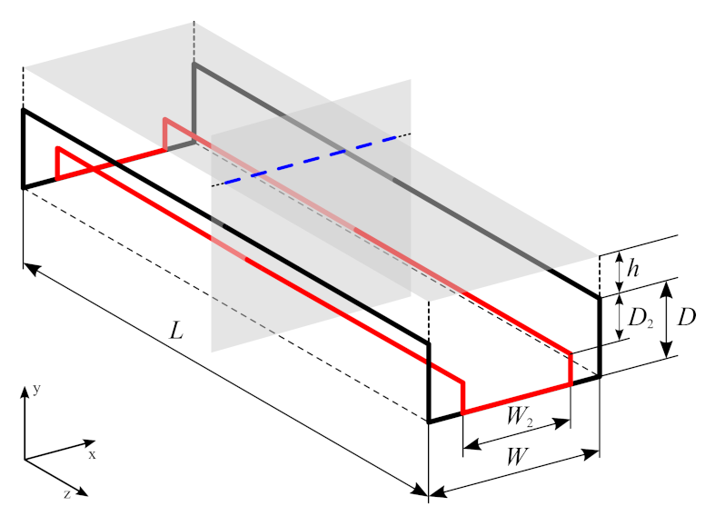
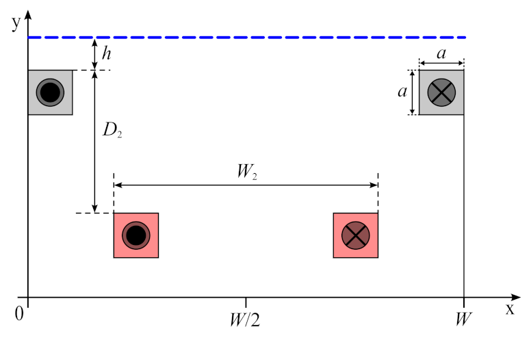
The intersection of the TX coil with the xy plane (vertical grey surface), shown in Figure 1, forms four cross-sections representing the position of the TX coil layers. The intersection of the charging plane and the xy plane in Figure 1 is the transverse line, which we refer to as the charging line in the following. The corresponding two-dimensional representation of the TX coil is shown in Figure 2. The cross-sections of the coil layers are simplified as squares. The two upper squares correspond to the first coil layer, while the two lower squares correspond to the second coil layer. The current directions in both coil layers are indicated by cross and dot symbols within the squares.

The charging line in Figure 2 corresponds to the charging plane of Figure 1, so the magnetic field intensity at charging line is relevant to the 2D optimization process. The following dot product is used to calculate the y-component of the magnetic field intensity:

$$H_y=\overrightarrow{H}·\overrightarrow{n},$$

(1)

where $\overrightarrow{H}$ is the magnetic field intensity vector (both the x and y components) and $\overrightarrow{n}$ is the unit vector parallel with the y axis.

Each of the squares in Figure 2 has the same area, and the square side a is equal to 2 mm. The transfer distance h was set to be constant and equal to 30 mm during the optimization process. The width of the first coil layer W was set to 280 mm. This width W has been found to be appropriate for a 3D coil made of two layers [17]. The first coil layer was included in the 2D optimization, but the positions of the squares representing it had a fixed position. The position of the squares of the second coil layer is defined by the decision variables D₂ and W₂. The mathematical notation of the 2D optimization problem follows:

$$f\left(\overrightarrow{X}\right)\to max.,$$

(2)

subject to the constraints:

$$g_j\left(\overrightarrow{X}\right)=0,$$

(3)

$$h_k\left(\overrightarrow{X}\right)\le 0,$$

(4)

where $\overrightarrow{X}$ is a vector of decision variables $\overrightarrow{X}$ = [x₁, ..., x_n]. The objective of the optimization was to maximize the average magnetic field intensity across the charging line and to maximize the section of the charging line where the homogeneous condition is satisfied. The average magnetic field intensity across the charging line is calculated as follows:

$$H_{ymean}=\frac{{\int }_0^W{H}_{y}dx}{W}.$$

(5)

The magnetic field intensity was observed at 1000 points over the entire charging line. The constraint in Equation (4) is expressed in the following two inequality constraints, Equations (6) and (7). The homogeneity criterion is predefined in terms of the maximum magnetic field intensity $\left(H_{ymax}\right)$ at the charging line:

$$H_y\le H_{ymax}.$$

(6)

Moreover, a homogeneous section of the charging line was characterized by a magnetic field intensity greater than or equal to 90% of $H_{ymax}$:

$$H_y\ge 0.9H_{ymax}.$$

(7)

To investigate the distribution of the magnetic field intensity distribution across the charging line, two 2D coil models were simulated in Ansys Maxwell. The 2D model of the flat rectangular coil consisted of only two squares (upper squares in Figure 2). Another 2D model corresponded to the coil optimized in [17], shown in Figure 2. The width of the 2D model of the rectangular coil corresponded to the width of the 2D model of the coil optimized in [17]. The transfer distance and currents were the same for both 2D models.

In Figure 3, three different distributions of the magnetic field intensity across the charging line are shown, an ideal coil, a rectangular coil, and the coil optimized in [17]. It is not possible to obtain an ideal distribution of the magnetic field intensity across the charging line that is as wide as the TX coil. Compared to a rectangular coil that does not produce a homogeneous section (concave distribution), the coil optimized in [17] provides a higher average magnetic field intensity, as well as a homogeneous section that occupies 85.14% of the length of the charging line.

Although the coil proposed in [17] produces a homogeneous section across more than 85% of the length of the charging line, there is a tendency to further develop the performance of such a coil shape. A higher percentage of the homogeneous section, a higher average magnetic field intensity across the homogeneous section, and a lower coil profile (lower D₂ and D from Figure 1) are the characteristics of an improved coil.

In [17], the same current flows through both layers, which allows defining the current distribution between the layers as the ratio r = I₁/I₂ = 1, where I₁ is the current of the first coil layer and I₂ is the current of the second coil layer. It was assumed that different r contribute to higher coil performance. Before the optimization process, I₁ and I₂ were set as integers, since the ratio r was then practically feasible. In practice, the number of turns of the first coil layer to the number of turns of the second coil layer is equal to the current distribution. Therefore, the number of turns of the coil layers could determine the current distribution.

GA optimization was performed using the Ansys Maxwell software Optimetrics tool. The cost function is defined as:

$$f\left(\overrightarrow{X}\right)=\left[1-\left(H_{ymax}\left(\overrightarrow{X}\right)-H_{ymean}\left(\overrightarrow{X}\right)\right)\right]·H_{ymean}\left(\overrightarrow{X}\right),$$

(8)

and the optimal solution is the maximum value of the cost function (best-fit individual). The maximum number of 250 generations was set as the termination criterion for the optimization process. Roulette selection was used. The vector $\overrightarrow{X}$ = [D₂,W₂] represents an individual in the population. The constraints on the decision variables are as follows:

$$3\le D_2\le 127\left(\mathrm{mm}\right),$$

(9)

$$5\le W_2\le 280\left(\mathrm{mm}\right).$$

(10)

The box constraints from Equations (9) and (10) define the search space of variables D₂ and W₂. The lower limit of the variable D₂ was set to 3 mm to avoid overlapping with the squares of the upper coil layer from Figure 2. The upper limit of the variable D₂ was set to 127 mm, which corresponds to the values of the variable D₂ observed in [17]. The lower limit of the variable W₂ was set to 5 mm to avoid overlapping the two lower squares from Figure 2, while the upper limit was set to 280 mm, corresponding to the width of the first coil layer W. The width of the second coil layer W₂ should be smaller than the width of the first coil layer W to compensate for the concave magnetic field intensity distribution of the single rectangular coil in Figure 3. The overlapping of any squares from Figure 2 in the Ansys Maxwell software immediately stops the optimization process.

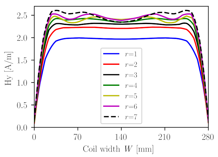
First, it was determined that the current distribution between layers should be such that the current of the first coil layer is greater than the current of the second coil layer (r is a positive integer). If this is not the case, the variable D₂ becomes larger and the coil profile is not reduced. In the simulations, different current distributions between the coil layers (different r) were set so that the sum of the currents was equal to the fixed value. For example, when r = 1, I₁ = 500 mA and I₂ = 500 mA, while for r = 3, I₁ = 750 mA and I₂ = 250 mA.

The variables D₂ and W₂ were optimized for each integer r in the range from one to seven, and the corresponding magnetic field intensity distributions are shown in Figure 4. The larger r is, the larger is also the magnetic field intensity across the charging line. Furthermore, the magnetic field intensity within the homogeneous section was more oscillatory as r increased. Moreover, in the case of r = 7 (dashed black line), the magnetic field intensity distribution did not exhibit a homogeneous section because the magnetic field intensity at the central position (W = 140 mm) was less than 90% of the maximum magnetic field intensity at the side position. It can be concluded that an optimization with r > 6 cannot fulfill the condition of homogeneity.

More detailed GA-optimized coil properties are shown in

Table 1. Comparison of the optimized coil characteristics for different current distributions.

r	Optimization Method	D2 (mm)	W2 (mm)	Hymean_hs (A/m)	Homogeneous Section (%)	Transfer Distance (mm)	FoM (A/m)	Calculated Value of Equation (8)
1 (Ref. [17])	Trial and error	56	196	2.06	85.14	24.6	175.39	N.A.
1	GA	58.71	212.42	1.97	80.42	30	158.43	1.493
2	GA	38.14	174.29	2.21	82.62	30	182.59	1.652
3	GA	27.14	150.98	2.30	84.32	30	193.94	1.754
4	GA	16.83	154.44	2.39	84.69	30	202.41	1.795
5	GA	8.82	135.76	2.41	85.39	30	205.79	1.761
6	GA	3.62	143.93	2.46	85.20	30	209.59	1.797
7	GA	3.62	154.55	/	/	30	/	1.721

. A higher r resulted in a smaller D₂, a wider homogeneous section, and a higher H_ymean, which were the optimization goals. The variable W₂ is not directly related to the reduction of the coil profile, but it is also important in the optimization process to obtain the right coil design. It was necessary to introduce a figure of merit (FoM) to compare the solutions for different r:

$$FoM=\mathrm{homogeneous}\sec \mathrm{tion}·H_{ymean\_hs}.$$

(11)

H_{ymean_hs} is the average value of the magnetic field intensity calculated only for the homogeneous section of the charging line. For each r value, FoM was calculated, and the highest value was for r = 6. Moreover, during the optimization, the minimum value of the variable D₂ was reached when r was set to six. Therefore, the following 3D optimization was performed with the predefined r = 6.

3.3. 3D Optimization

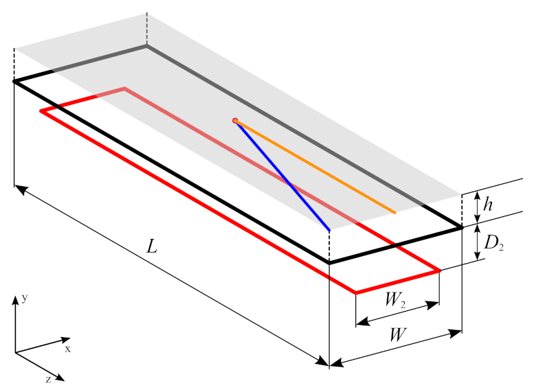
Although the optimization of the 3D model of the TX coil took more time, it was necessary because of the 3D properties of the optimized coil. The 3D model of the two-layer TX coil was also created in the Ansys Maxwell software. Based on the 2D optimization solution, the current of the first coil layer was set six-times larger than the current of the second coil layer. In this step, the two layers were flat rectangular and the values of the variables of the second coil layer (D₂ and W₂) corresponded to the optimal values obtained in the 2D optimization for r = 6.

The 3D model of the TX coil with two rectangular layers with the optimized variables D₂ and W₂ is shown in Figure 5. The basic idea of the 2D model optimization was that the homogeneous magnetic field intensity distribution at the charging line (transverse blue line in Figure 1) was preserved along most of the TX coil length L. To verify this assumption, the magnetic field intensity distribution along the longitudinal and diagonal lines (orange and blue, respectively) in the charging plane was observed (see Figure 5).

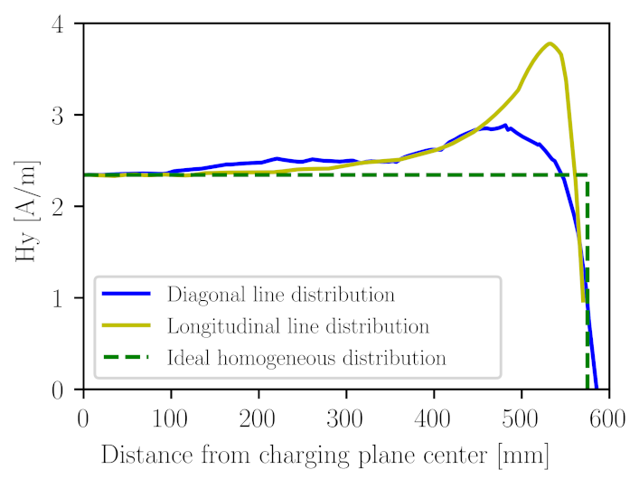
Combined with the ideal homogeneous magnetic field intensity distribution, the magnetic field intensity distributions along the longitudinal and diagonal lines are shown in Figure 6. Due to the symmetry of the coil with respect to the xy and yz planes, the magnetic field intensity distribution was observed only in half of the charging plane. Although the TX coil variables D₂ and W₂ were set to optimal values, the magnetic field intensity distribution was characterized by peaks near the TX coil end. As the distance from charging plane center increased, the magnetic field intensity also increased. This trend in magnetic field intensity produced a nonhomogeneous magnetic field intensity distribution.

To maintain a homogeneous distribution along most of the coil length L, the authors in [17] proposed to fold the coil ends downward, as shown in Figure 1. Their optimal coil was folded down to the depth D = 11.8 cm. The 3D model of the TX coil shown in Figure 1 was created in Ansys Maxwell, with values for D₂ and W₂ set according to the 2D optimization solution for r = 6. The adapted cost function was applied:

$$f\left(\overrightarrow{X}\right)=\left[1-\left(H_{ymax\_S}\left(\overrightarrow{X}\right)-H_{ymean\_S}\left(\overrightarrow{X}\right)\right)\right]·H_{ymean\_S}\left(\overrightarrow{X}\right),$$

(12)

where the vector $\overrightarrow{X}$ = [D] represents an individual in the 3D model GA optimization. The range for finding the optimal value of the decision variable D was set to:

$$8.12\le D\le 125\left(\mathrm{mm}\right).$$

(13)

The lower bound of the variable D was set with respect to the previous optimization solutions. The optimal value of the variable D₂ was 3.62 mm, and the square wire of the coil layers in the 3D model had a side of 2 mm. Therefore, adding the optimal value of D₂, the two 2 mm sides of the first and second coil layers, and the 0.5 mm distance between them, we obtained a lower limit of 8.12 mm. The upper limit of the variable D was set to 125 mm, which corresponds to the values of the variable D observed in [17].

The magnetic field intensity quantities used to form the cost function (12) were calculated with respect to the charging plane 30 mm above the TX coil. The Fields Calculator tool of the Ansys Maxwell software was used to calculate the maximum value of the magnetic field intensity in the charging plane, H_{ymax_S}. The average value of the magnetic field intensity across the charging plane is calculated as follows:

$$H_{ymean\_S}=\frac{{\int }_0^S{H}_{y}dxdy}{S}$$

(14)

Similar to the optimization of the 2D model, the goal of the optimization of the 3D model was to maximize the area of the charging plane in which a homogeneous magnetic field intensity distribution was achieved, while keeping H_{ymean_S} as large as possible within this area of the charging plane.

Since the widths (W and W₂), length L, and vertical distance between the layers of the coil (D₂) were given in this step of the optimization, the variable D should be optimized. The maximum number of 50 generations was set as the criterion for the end of the optimization process. The roulette selection was switched on.

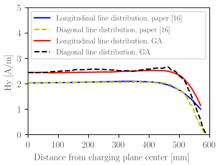
The maximum value of the cost function (Equation (12)) in the GA optimization was reached for D = 8.39 cm. Therefore, the GA-optimized coil characteristic had a lower profile in comparison to the coil proposed in [17]. The magnetic field intensity distribution along the longitudinal and diagonal lines of the charging plane is shown in Figure 7. The field distribution of the coil optimized by GA and the coil optimized in [17] developed a similar pattern. However, the difference in the field distribution was that the GA-optimized coil produced a higher magnetic field intensity along the lines. Therefore, the GA-optimized coil produced a higher average magnetic field intensity.

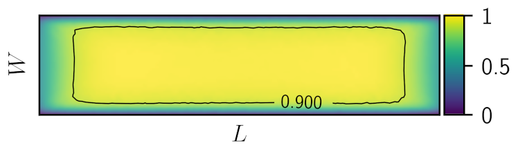
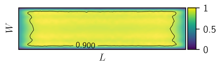
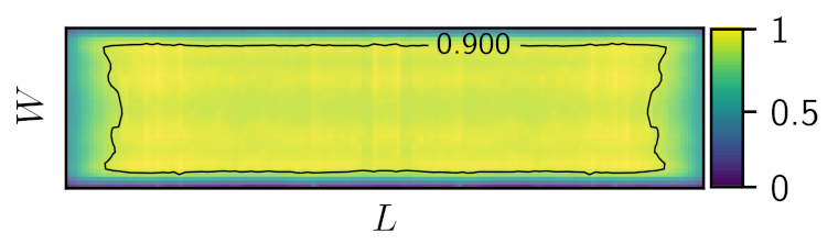
The simulation results of the distribution of the magnetic field intensity in the charging plane for the coil optimized in [17] and the GA-optimized coil are shown in Figure 8 and Figure 9, respectively. The magnetic field intensity values were normalized with respect to H_{ymax_S}. The homogeneous area was surrounded by a black line representing the boundary. Namely, outside the homogeneous area, the magnetic field intensity was less than 0.9H_{ymax_S}. The homogeneous area was characterized by a magnetic field intensity of 0.9H_{ymax_S} or more.

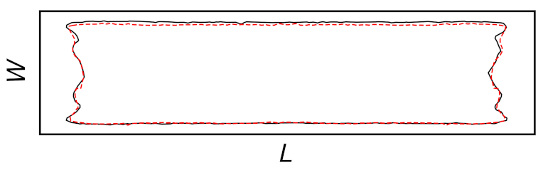
The homogeneous area of the GA-optimized coil was significantly larger than the corresponding homogeneous area of the coil optimized in [17]. The homogeneous area of the GA-optimized coil was wider and extended more toward the ends of the charging plane. It was calculated that the coil optimized in [17] generated a homogeneous area occupying 62.53% of the surface of the charging plane. On the other hand, the GA-optimized coil produced a homogeneous area occupying 70.33% of the surface of the charging plane. Due to the larger homogeneous area, higher average magnetic field intensity, and lower coil profile, the GA-optimized coil was more suitable than the coil optimized in [17].

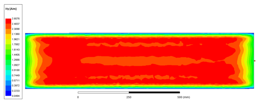
The nephogram of magnetic field intensity in the charging plane generated by the optimized 3D coil is shown in Figure 10. The color rule (legend) in Figure 10 indicates the magnetic field intensity at a particular point of the charging plane.

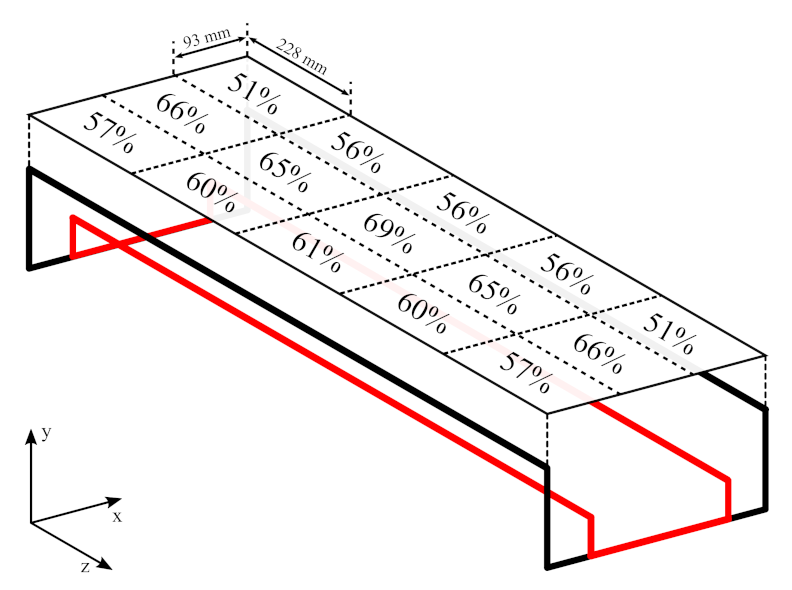
To determine the stability of the power transfer efficiency for different RX coil positions in the charging plane, a rectangular RX coil (22.8 × 9.3 cm) was created in Ansys Maxwell. The first part of the simulations consisted of calculating the self-inductance of the TX coil and the RX coil, the mutual inductance among them, and the coupling coefficient k for 15 different RX coil positions in the charging plane. Based on these simulation results, the parallel-series topology of the WPT system was used to calculate the power transfer efficiency for each RX coil position. Figure 11 shows the transfer efficiency for 15 different positions of the RX coil in the charging plane. The highest efficiency of 69% was achieved when the RX coil was in the middle of the charging plane. The degradation of the efficiency for the RX coil placed at the sides of the charging plane was expected due to the nonhomogeneity of the intensity of the magnetic field in the corresponding areas of the charging plane (see Figure 9 and Figure 10). However, the transfer efficiency was stable in the areas of the charging plane where the magnetic field intensity distribution was homogeneous. The lowest power transfer efficiency (51%) was calculated when the RX coil was placed at the corner of the charging plane where the magnetic field intensity was most nonhomogeneous compared to other areas of the charging plane. In summary, the power transfer efficiency of the proposed coil remained stable, so the minimum power transfer efficiency was 73.9% of the middle position efficiency regardless of the RX coil position.

4. Measurements

The GA-optimized coil was constructed, and measurements of the magnetic field intensity distribution in the charging plane were performed to verify the optimization solutions. The length of the two coil layers L was the same, 114 cm. The width of the first coil layer W was set to 28 cm, while the width of the second coil layer W₂ was set to 14.4 cm. The remaining coil dimensions, D and D₂, were consistent with the optimization solutions. Therefore, the value of D was 8.4 cm and D₂ was equal to 3.6 mm.

The coil optimized in this way was installed in a wooden frame, which kept the wires of the coil in a certain position and ensured a transfer distance of 30 mm. Round iron wire with a diameter of 4 mm was used to complete both layers of the coil. Figure 12 shows the bottom view of the fabricated coil.

The coil shown in Figure 12 consisted of one turn per layer, and each layer was considered as a single coil. For measurement purposes, the coil layers were connected in parallel. The resistor, R₁ = 1 kΩ, was connected in series with the first coil layer, L₁. The six-times larger resistor, R₂, was connected in series with the second coil layer, L₂ (Figure 13). In this way, an optimal current distribution between the coil layers was achieved. Such a circuit arrangement with resistors is not practical for wireless power transfer because of the power dissipation. The actual GA-optimized TX coil with two layers connected in series for efficient WPT did not contain resistors for the current distribution. Instead, the number of turns of the first coil layer should be six-times larger than the number of turns of the second coil layer to achieve the optimal current distribution (r = 6). However, the higher precision in the manufacture of the coil with one turn per layer and resistors that ensure optimal current distribution are sufficient for magnetic field measurements.

Magnetic field measurements were performed using the SPECTRAN NF-5035 analyzer. An external sensor was connected to the SMA input. When the external sensor was applied, the voltage was measured and shown on the analyzer display. The voltage induced in the sensor was proportional to the rate of change of the magnetic flux; therefore, magnetic field measurements can be made in this way. The fabricated coil was excited by an Agilent 33250A signal generator (s.g.), which produced a sine wave of 20 V (peak-to-peak) and a 1.5 MHz frequency. The measurement setup is shown in Figure 13.

The magnetic field measurements were made at specific points of the charging plane. The symmetry of the coil with respect to the xy and yz planes (seen in Figure 1) was the basis for assuming that the distribution of the magnetic field intensity at one half of the charging plane should be the same at the other half of the charging plane. Therefore, the measurements were made on one half of the charging plane. The measurements were performed over the entire width W and half of the length L/2 of the charging plane. The measurement points were aligned along parallel longitudinal lines (as the orange line in Figure 5) that were 1 cm apart. Thus, there were 29 parallel longitudinal lines covering the entire width of the charging plane (W = 28 cm). The distance between the adjacent measurement points on the same longitudinal line was set to 1 cm. Accordingly, there were 58 measurement points on each longitudinal line. In this way, a grid of 1682 (29 × 58) measurement points was created

The measurement results are shown in Figure 14. The measured values were normalized with respect to the maximum value of the induced voltage. The homogeneous area is surrounded by a black line representing the boundary. Namely, outside the homogeneous area, the induced voltage was lower than 0.9 of the maximum value of the induced voltage. The manufactured coil was calculated to generate a homogeneous area occupying 67.78% of the surface of the charging plane.

The outlines of the homogeneous area defined by the simulation and the measurement results are shown in Figure 15. The homogeneous area of the measurement results (area inside the red dashed curve) occupied 2.55% less area of the charging plane than the homogeneous area of the simulation results (area inside the black solid curve). Not only did the measurement results show accurate numerical agreement with the simulation results, but also the shape of the homogeneous area obtained by the measurements agreed with the homogeneous area obtained by the simulations.

The measured characteristics of the various optimized TX coil designs that produced a homogeneous area in the charging plane are listed in

Table 2. Comparison of various optimized TX coils’ characteristics.

Ref.	Structure	TX Coil (cm2) or (cm3)	r (%)	h (mm)	Homogeneous Area (Measured)
[2]	Printed Circular Spiral	${10}^2\times \pi$	30	15	~64%
[4]	Planar Square	20 × 20	20	1	~36%
[12]	Planar Square	20 × 20	20	50	~51.8%
[14]	Planar Square	80 × 80	9.6	100	~42.3%
[16]	3D Rectangular	22 × 18 × 2	20	0.5	~32%
[17]	3D Rectangular	114 × 28 × 12	10	30	~55.3%
[20]	Planar Square	20 × 20	20	150	~48%
[21]	Planar Square	50 × 50	7.2	18	~49%
[22]	Planar Square	31.5 × 31.5	2	30	~49%
This paper	3D Rectangular	114 × 28 × 9	10	30	~67.8%

. Compared to other TX coil properties from Table 2, the coil optimized in this work produced a larger fraction of the homogeneous area in the charging plane.

5. Conclusions

A current distribution approach for a two-layer rectangular 3D TX coil in an MCR-WPT system was proposed, with the aim of increasing the area of the homogeneous magnetic field intensity distribution and decreasing the coil profile (coil height). The coil layer arrangement and current distribution were optimized using a genetic algorithm. The optimization was performed using the Ansys Maxwell Optimetrics tool. It was found that the optimal current distribution between the coil layers should be such that the current ratio in the coil layers is six to one. The simulation results obtained with the Ansys Maxwell software were verified by measurements on a coil prototype. The main achievements of the coil optimized in this work compared to other optimized TX coils (including our previous work) were: a larger fraction of the homogeneous area, a lower profile, and a higher average magnetic field intensity within the homogeneous area. The fraction of the homogeneous area was increased by 12.5% for the same charging plane, and the coil depth was reduced by 29% (from 11.8 cm to 8.4 cm). The average magnetic field intensity within the homogeneous area was increased by 25%. However, the distribution of the magnetic field intensity within the homogeneous area was not as uniform as that achieved in the previous work. Further research should therefore aim to make the distribution flatter while maintaining or even improving the properties of the coil.

References

1. Li, Y.; Zhao, J.; Yang, Q.; Liu, L.; Ma, J.; Zhang, X. A Novel Coil With High Misalignment Tolerance for Wireless Power Transfer. IEEE Trans. Magn. 2019, 55, 2800904. [Google Scholar] [CrossRef]
2. Xu, Q.; Hu, Q.; Wang, H.; Mao, Z.H.; Sun, M. Optimal Design of Planar Spiral Coil for Uniform Magnetic Field to Wirelessly Power Position-Free Targets. IEEE Trans. Magn. 2021, 57, 4000709. [Google Scholar] [CrossRef]
3. Liu, X.; Hui, S.Y. Optimal Design of a Hybrid Winding Structure for Planar Contactless Battery Charging Platform. IEEE Trans. Power Electron. 2008, 23, 455–463. [Google Scholar] [CrossRef]
4. Casanova, J.J.; Low, Z.N.; Lin, J.; Tseng, R. Transmitting coil achieving uniform magnetic field distribution for planar wireless power transfer system. In Proceedings of the 2009 IEEE Radio and Wireless Symposium, San Diego, CA, USA, 18–22 January 2009; pp. 530–533. [Google Scholar] [CrossRef]
5. Yinliang, D.; Yuanmao, S.; Yougang, G. Design of coil structure achieving uniform magnetic field distribution for wireless charging platform. In Proceedings of the 2011 4th International Conference on Power Electronics Systems and Applications, Hong Kong, China, 8–10 June 2011; pp. 1–5. [Google Scholar] [CrossRef]
6. Kim, J.; Son, H.C.; Park, Y.J. Multi-loop coil supporting uniform mutual inductances for free-positioning WPT. Electron. Lett. 2013, 49, 417–419. [Google Scholar] [CrossRef]
7. Waffenschmidt, E. Homogeneous Magnetic Coupling for Free Positioning in an Inductive Wireless Power System. IEEE J. Emerg. Sel. Top. Power Electron. 2015, 3, 226–233. [Google Scholar] [CrossRef]
8. Yeo, T.; Kim, D.; Chae, S.C.; Khang, S.; Yu, J. Design of free-positioning wireless power charging system for AAA rechargeable battery. In Proceedings of the 2016 46th European Microwave Conference (EuMC), London, UK, 4–6 October 2016; pp. 759–762. [Google Scholar] [CrossRef]
9. Shen, L.; Tang, W.; Xiang, H.; Zhuang, W. Uniform magnetic field of the planar coil with new winding structure for displacement-insensitive WPT. In Proceedings of the 2014 IEEE International Conference on Communiction Problem-Solving, Beijing, China, 5–7 December 2014; pp. 394–396. [Google Scholar] [CrossRef]
10. Yang, Y.; Kuang, X.; Yang, P.; Jing, Y.; Su, X.; Cheng, Y. Parallel connected transmitting coil for achieving uniform magnetic field distribution in WPT. In Proceedings of the 2015 IEEE 16th International Conference on Communication Technology (ICCT), Hangzhou, China, 18–20 October 2015; pp. 529–532. [Google Scholar] [CrossRef]
11. Chung, C.H.; Yang, C.L. Novel Parallel Serpentine Coils with High Lateral Misalignment Tolerance and Power Transfer Efficiency Optimization. In Proceedings of the 2020 IEEE Wireless Power Transfer Conference (WPTC), Seoul, Korea, 15–19 November 2020; pp. 480–483. [Google Scholar] [CrossRef]
12. Wang, S.; Hu, Z.; Rong, C.; Lu, C.; Chen, J.; Liu, M. Planar Multiple-Antiparallel Square Transmitter for Position-Insensitive Wireless Power Transfer. IEEE Antennas Wirel. Propag. Lett. 2018, 17, 188–192. [Google Scholar] [CrossRef]
13. Kim, T.; Yun, G.; Lee, W.Y.; Yook, J. Asymmetric Coil Structures for Highly Efficient Wireless Power Transfer Systems. IEEE Trans. Microw. Theory Tech. 2018, 66, 3443–3451. [Google Scholar] [CrossRef]
14. Zhang, Y.; Wang, L.; Guo, Y.; Zhang, Y. Optimisation of planar rectangular coil achieving uniform magnetic field distribution for EV wireless charging based on genetic algorithm. IET Power Electron. 2019, 12, 2706–2712. [Google Scholar] [CrossRef]
15. Bilandžija, D.; Vinko, D.; Biondić, I. Achieving Uniform Magnetic Field with Rectangular Coil in Wireless Power Transmission System. In Proceedings of the 2019 International Symposium ELMAR, Zadar, Croatia, 23–25 September 2019; pp. 179–182. [Google Scholar] [CrossRef]
16. Lee, W.S.; Lim Lee, H.; Oh, K.S.; Yu, J.W. Uniform magnetic field distribution of a spatially structured resonant coil for wireless power transfer. Appl. Phys. Lett. 2012, 100, 214105. [Google Scholar] [CrossRef] [Green Version]
17. Vinko, D.; Bilandžija, D.; Mandrić Radivojević, V. Optimization of a Two-Layer 3D Coil Structure with Uniform Magnetic Field. Wirel. Power Transf. 2021, 2021, 6303628. [Google Scholar] [CrossRef] [PubMed]
18. Sasatani, T.; Narusue, Y.; Kawahara, Y. Genetic Algorithm-Based Receiving Resonator Array Design for Wireless Power Transfer. IEEE Access 2020, 8, 222385–222396. [Google Scholar] [CrossRef]
19. Ansys® Electronics Desktop, Release 19 4, Maxwell Help, Optimetrics, Optimization, Genetic Algorithm, ANSYS, Inc.: Canonsburg, PA, USA, 2019.
20. Qiu, C.; Chau, K.T.; Chunhua, L.; Ching, T.; Zhang, Z. Modular inductive power transmission system for high misalignment electric vehicle application. J. Appl. Phys. 2015, 117, 17B528. [Google Scholar] [CrossRef] [Green Version]
21. Li, J.; Sun, J.; Qin, R.; Costinett, D. Transmitter Coil Design for Multi-load Wireless Power Transfer Systems. In Proceedings of the 2020 IEEE Energy Conversion Congress and Exposition (ECCE), Detroit, MI, USA, 11–15 October 2020; pp. 1032–1038. [Google Scholar] [CrossRef]
22. Zhang, C.; Wang, W.; Xu, C.; Yang, J. Research on Uniform Magnetic Field Compensation Structure of Array Circular Coils for Wireless Power Transfer. IEEE Trans. Magn. 2021, 57, 8600205. [Google Scholar] [CrossRef]
Figure 1. Basic coil design.
Energies 15 01381 g001
Figure 2. Two-dimensional representation of the TX coil.
Energies 15 01381 g002
Figure 3. Simulation results: comparison of the magnetic field intensity distributions.
Energies 15 01381 g003
Figure 4. Magnetic field intensity distributions for optimized variables D2 and W2 with different current distributions.
Energies 15 01381 g004
Figure 5. Three-dimensional model of two rectangular layer TX coil.
Energies 15 01381 g005
Figure 6. Simulation results of magnetic field intensity distribution along the longitudinal and diagonal line for two rectangular layer TX coils.
Energies 15 01381 g006
Figure 7. Simulation results of the magnetic field intensity distribution along the longitudinal and diagonal line.
Energies 15 01381 g007
Figure 8. Simulation results of the normalized magnetic field intensity distribution in the charging plane of the coil optimized in [17].
Energies 15 01381 g008
Figure 9. Simulation results of the normalized magnetic field intensity distribution in the charging plane of the GA-optimized coil.
Energies 15 01381 g009
Figure 10. Ansys Maxwell simulation results of the magnetic field intensity distribution in the charging plane of the GA-optimized coil.
Energies 15 01381 g010
Figure 11. Simulation results of the power transfer efficiency for different RX coil positions in the charging plane (Rload = 5 Ω).
Energies 15 01381 g011
Figure 12. Fabricated coil, bottom view.
Energies 15 01381 g012
Figure 13. Measurement setup and equivalent scheme of the driven circuit.
Energies 15 01381 g013
Figure 14. Measurement results of normalized magnetic field intensity distribution in the charging plane of the GA-optimized coil.
Energies 15 01381 g014
Figure 15. Outline of the homogenous area in the charging plane for the simulation and measurement results.
Energies 15 01381 g015