Novel Mathematical Design of Triple-Tuned Filters for Harmonics Distortion Mitigation

Abstract

The design of AC filters must meet the criteria of harmonic distortion mitigation and reactive power support in various operating modes. The stringent reactive power-sharing requirements currently lead to sophisticated filter schemes with high component ratings. In this regard, triple-tuned filters (TTFs) have good potential in harmonic mitigation of a broad range of harmonics. In the literature, the TTF design has been presented using a parametric method, assuming that the TTF is equivalent to a three-arm single-tuned filter (TASTF). However, no direct methods of designing it or finding its optimal parameters have been provided. This paper presents novel mathematical designs of TTFs. Three different design methods are considered—the direct triple-tuned filter (DTTF) design method, as a TASTF, and a method based on the equivalence between the two design methods called the equivalence hypothesis method to design the triple-tuned filter (EHF). The parameters of the three proposed design methods are optimized based on the minimization of a proposed multi-objective function using a recent metaheuristic algorithm called artificial rabbits optimization (ARO) to mitigate harmonics, improve power quality, and minimize power losses in an exemplary system presented in IEEE STD-519. Further, the system’s performance has been compared to the system optimized by the ant lion optimizer (ALO) and whale optimization algorithm (WOA) to validate the effectiveness of the proposed design. Simulation results emphasized harmonics mitigation in the system, the system losses reduction, and power quality improvement with lower reactive power filter ratings than conventional single and double-tuned filters.

1. Introduction

Recently, numerous power quality problems have spread due to the extensive use of electronic appliances, industrial applications, and renewable energy sources, as well as the increased use of electric vehicles. In terms of power quality, harmonics are produced by the increasing use of nonlinear loads in power systems, which adversely impacts how well these systems will function [1]. The primary concern for the distribution systems planners and operators is maintaining the system with high power quality levels, reducing electrical loss, and keeping the power factor within the desired limits. However, this is threatened by harmonics distortion because it increases system power losses and decreases transmission efficiency, in addition to overheating and reduced loading capacity in frequency-dependent components such as cables, transformers, and induction machines. Harmonics distortion also causes poor power factor levels, poor efficiency, reduced hosting capacity levels of distributed generation units in power systems, malfunction of protective relays and electronic circuits, and resonance problems among the inductive source impedance and shunt capacitors [2].

Passive filters are frequently employed to reduce the impacts of the increased harmonics due to their simple design, low price, excellent dependability, and ease of maintenance [3]. Also, they are commonly used in distribution systems for reactive power compensation and voltage support [4]. On the one hand, harmonic distortion at specific harmonic orders can be reduced using tuned filters, such as single-tuned or double-tuned filters, as they provide better harmonic mitigation than damped filters; however, they may suffer from parameter variations and resonance occurrence. On the other hand, compared to tuned filters, damped filters offer good harmonic suppression and improved harmonic resonance damping capability [5].

Many approaches have been presented in the literature to mitigate harmonics and reduce distortions in modern power and energy systems. Single-tuned filters (STFs) are frequently employed to mitigate an individual distortion provided by a specific harmonic frequency, but they perform poorly in systems with high harmonic distortion [6,7]. In order to reduce multiple harmonic frequencies, double-tuned filters (DTFs) or multi-arms single-tuned filters (MASTFs) can be utilized [4,5]. DTFs have almost the same performance but at a cheaper cost. It is possible to design a DTF in three ways: by using MASTF directly, considering it as two parallel STFs, or by evaluating the characteristics of the previous two designs with the assumption that their harmonic impedances are equal. These techniques are presented in [8] to eliminate system harmonics and enhance the power quality performance of the studied system.

In this regard, a triple-tuned filter (TTF) can simultaneously lessen the harmonic distortion of three frequencies. It has been applied in some projects in China, Thailand, and others. However, it was noted that they empirically designed it because of the mathematical complexity of finding its parameters.

In the literature, few publications presented the design of TTF by considering its parameters to be the same as three parallel STFs. For instance, in [9], the TTF was presented as three STF branches in the HVDC schemes—EGAT-TNB 300 MW HVDC Interconnection and Moyle Interconnector, in which the experience gained during the commissioning tests and the subsequent commercial operation were reported in [9]. A three-tuned filter to minimize harmonics in a power system was presented in [10] while presenting an analog equivalent design to three parallel STFs. Their filter design performed better than STFs in mitigating harmonics and reducing power loss, with low space occupation and price.

In [11], the authors suggested that the design of double and triple-tuned filters include splitting the filter into two or three STFs to simplify the design process. Also, in [12], the author presented a method for designing a filter group based on distributing the reactive power among filters in the group.

The study in [13] provided a comparative assessment of five widely known passive harmonic filters, STF, DTF, TTF, damped DTF, and C-type filters, regarding their contribution to the loading capability of the transformers under non-sinusoidal conditions. Only the equivalent impedances of these filters were considered in the presented design, with no mathematical design of the TTF. It was clearly observed from the results obtained for the investigated distorted system with its nonlinear loads and background voltage distortion that the TTF outperformed the other considered filters in terms of the transformer’s loading capability improvement. In addition, an analytical optimization of the filtration efficiency of a group of single-branch filters was presented in [14] to design filters with the minimized sum of various harmonic reduction metrics to improve the power quality level of the system. To sum up, due to the problematic design of the TTF, there was no way to develop and improve the performance of this type of filter using a direct design method in the literature.

To redress this gap, this paper presents a novel mathematical formulation of the TTF in detail using three design models: direct design, three arms of a single-tuned filter (TASTF), and their equivalence hypothesis. Further, the filter parameters are obtained using the bio-inspired meta-heuristic artificial rabbits optimization (ARO) algorithm to minimize power losses and enhance the power quality performance of the studied system. The results of the proposed filter schemes are obtained using ARO and compared to those obtained using the ant-lion optimizer (ALO) and the whale optimization algorithm (WOA) to demonstrate the effectiveness of the used algorithm.

The rest of the article is structured as follows. The design methodologies of the TTF are presented in detail in Section 2. The system description, problem formulation, objective function proposed, and problem constraints are addressed in Section 3. The three employed optimization techniques—ARO, ALO, and WOA—are presented in Section 4. The obtained results are presented and discussed in Section 5. Finally, Section 6 concludes the work and introduces recommendations and possible future works for this study.

2. Design Methodologies of Triple-Tuned Filters

The triple-tuned filter can be mathematically designed in three ways, the direct triple-tuned filter (DTTF) design method, as a TASTF, and a method based on the equivalence between the two design methods called the equivalence hypothesis method to design the triple-tuned filter (EHF). In this section, the three design techniques are discussed.

2.1. Mathematical Design for Three Arms of a Single-Tuned Filter

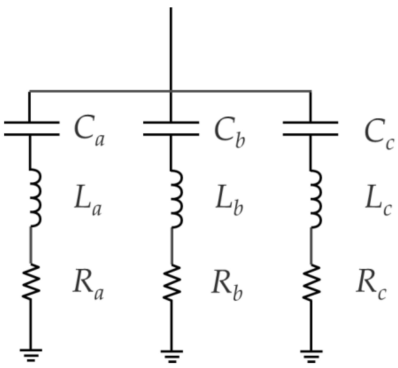
The three arms of a single-tuned filter (TASTF) rely on the basic structure of a single-tuned filter, as stated in [9,11,14], which consists of a series arrangement of an inductor L, capacitor C, and resistance R, as shown in Figure 1. For simplicity, one can consider the real part of the filter impedance equal to zero, i.e., R = 0. That will provide much more adequate tuned harmonic elimination characteristics and improve the system’s power quality.

The arms impedances $Z_a$, $Z_b$ and $Z_c$ can be calculated as follows:

$$Z_a(\omega )=j\left(\omega L_a-\frac{1}{\omega C_a}\right),$$

(1)

$$Z_b(\omega )=j\left(\omega L_b-\frac{1}{\omega C_b}\right),$$

(2)

$$Z_c(\omega )=j\left(\omega L_c-\frac{1}{\omega C_c}\right).$$

(3)

where C_a, L_a denote the capacitance and inductance of the first arm, C_b, L_b denotes the capacitance and inductance of the second arm, C_c, L_c denotes the capacitance and inductance of the third arm and ω denotes the angular frequency.

Each arm has its resonance frequency, so the TASTF has three resonance frequencies ω_ra, ω_rb, and ω_rc. At each resonance frequency, the impedance of the arm is equal to zero. Thus, the resonance frequencies can be represented as follows:

$${\omega }_{ra}=\frac{1}{\sqrt{L_a{C}_a}},$$

(4)

$${\omega }_{rb}=\frac{1}{\sqrt{L_b{C}_b}},$$

(5)

$${\omega }_{rc}=\frac{1}{\sqrt{L_c{C}_c}}.$$

(6)

These angular resonance frequencies can be written as a function of the fundamental frequency ω_f, as follows:

$${\omega }_{ra}=h_a{\omega }_f,$$

(7)

$${\omega }_{rb}=h_b{\omega }_f,$$

(8)

$${\omega }_{rc}=h_c{\omega }_f.$$

(9)

where h_a, h_b, h_c denote the harmonic tuning order.

The inductance of each filter’s branch can be obtained from (4)–(9) as follows:

$$L_a=\frac{1}{h_a^2{\omega }_f^2{C}_a},$$

(10)

$$L_b=\frac{1}{h_b^2{\omega }_f^2{C}_b},$$

(11)

$$L_c=\frac{1}{h_c^2{\omega }_f^2{C}_c}.$$

(12)

The total admittance of the TASTF can be obtained as follows:

$$\frac{1}{Z_f}=\frac{1}{Z_a}+\frac{1}{Z_b}+\frac{1}{Z_c}$$

(13)

From (1)–(3) and (10)–(12), the total admittance can be rewritten as:

$$\frac{1}{Z_f}=j{C}_a\frac{{h_a}^2{{\omega }_f}^2\omega }{{h_a}^2{{\omega }_f}^2-{\omega }^2}+j{C}_b\frac{{h_b}^2{{\omega }_f}^2\omega }{{h_b}^2{{\omega }_f}^2-{\omega }^2}+j{C}_c\frac{{h_c}^2{{\omega }_f}^2\omega }{{h_c}^2{{\omega }_f}^2-{\omega }^2}$$

(14)

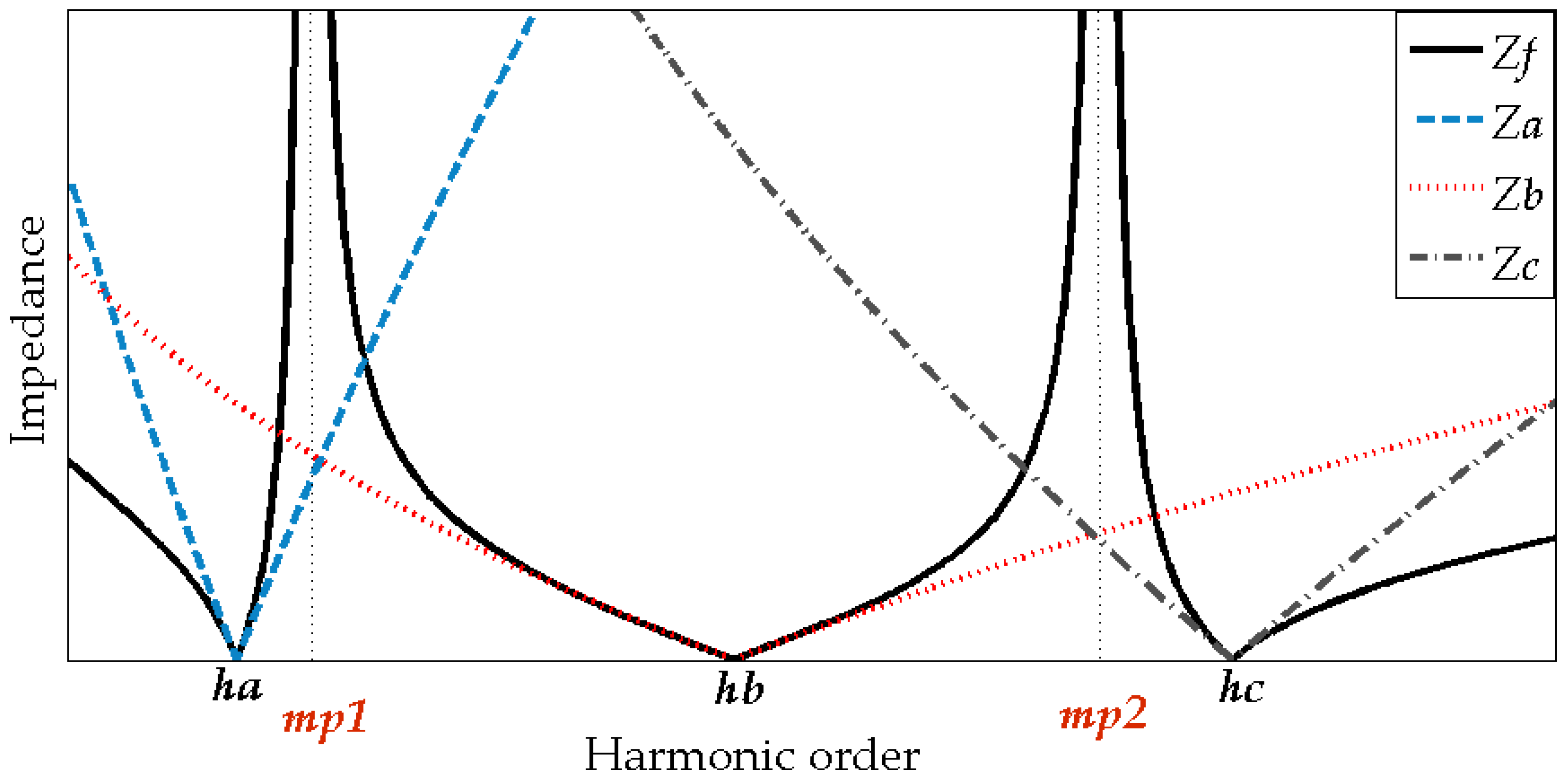
The TASTF impedance characteristic is illustrated in Figure 2. The impedance of the filter will be zero at the tuning frequencies ω_ra, ω_rb, and ω_rc in order to eliminate these harmonics. At the same moment, the impedance value at the parallel frequencies ω_p1 and ω_p2 will reach a maximum value. The parallel frequencies are represented as a function of the fundamental frequency.

$${\omega }_{p1}=m_{p1}{\omega }_f$$

(15)

$${\omega }_{p2}=m_{p2}{\omega }_f,$$

(16)

where m_p1 and m_p2 are the harmonic order of the parallel resonance frequency.

Based on the impedance characteristics of the TASTF, the capacitance of each branch can be calculated at the fundamental angular frequency ω_f, as follows:

$$Z_f({\omega }_f)=-j\frac{V_s^2}{Q_f}.$$

(17)

Substituting (17) into (14), thus:

$$\frac{1}{Z_f({\omega }_f)}=C_a\frac{{h_a}^2{{\omega }_f}^2{\omega }_f}{{h_a}^2{{\omega }_f}^2-{{\omega }_f}^2}+C_b\frac{{h_b}^2{{\omega }_f}^2{\omega }_f}{{h_b}^2{{\omega }_f}^2-{{\omega }_f}^2}+C_c\frac{{h_c}^2{{\omega }_f}^2{\omega }_f}{{h_c}^2{{\omega }_f}^2-{{\omega }_f}^2}=\frac{Q_f}{V_s^2}$$

(18)

Simplifying (18) will lead to the following equation:

$$C_a\frac{{h_a}^2}{{h_a}^2-1}+C_b\frac{{h_b}^2}{{h_b}^2-1}+C_c\frac{{h_c}^2}{{h_c}^2-1}=\frac{Q_f}{{\omega }_f{V}_s^2}$$

(19)

At the first parallel frequency, i.e., $\omega ={\omega }_{p1}$, the admittance $\frac{1}{Z_f({\omega }_{p1})}=0$, therefore:

$$C_a\frac{{h_a}^2{{\omega }_f}^2{\omega }_{p1}}{{h_a}^2{{\omega }_f}^2-{{\omega }_{p1}}^2}+C_b\frac{{h_b}^2{{\omega }_f}^2{\omega }_{p1}}{{h_b}^2{{\omega }_f}^2-{{\omega }_{p1}}^2}+C_c\frac{{h_c}^2{{\omega }_f}^2{\omega }_{p1}}{{h_c}^2{{\omega }_f}^2-{{\omega }_{p1}}^2}=0$$

(20)

Dividing (20) by ${\omega }_{p1}{{\omega }_f}^2$ and considering that $m_{p1}=\frac{{{\omega }_{p1}}^2}{{{\omega }_f}^2}$ will leads to:

$$C_a\frac{{h_a}^2}{{h_a}^2-{m_{p1}}^2}+C_b\frac{{h_b}^2}{{h_b}^2-{m_{p1}}^2}+C_c\frac{{h_c}^2}{{h_c}^2-{m_{p1}}^2}=0$$

(21)

At the second parallel frequency, $\omega ={\omega }_{p2}$, the admittance $\frac{1}{Z_f({\omega }_{p2})}=0$, therefore:

$$C_a\frac{{h_a}^2{{\omega }_f}^2{\omega }_{p2}}{{h_a}^2{{\omega }_f}^2-{{\omega }_{p2}}^2}+C_b\frac{{h_b}^2{{\omega }_f}^2{\omega }_{p2}}{{h_b}^2{{\omega }_f}^2-{{\omega }_{p2}}^2}+C_c\frac{{h_c}^2{{\omega }_f}^2{\omega }_{p2}}{{h_c}^2{{\omega }_f}^2-{{\omega }_{p2}}^2}=0$$

(22)

Dividing (22) by ${\omega }_{p2}{{\omega }_f}^2$ and considering that $m_{p2}=\frac{{{\omega }_{p2}}^2}{{{\omega }_f}^2}$;

$$C_a\frac{{h_a}^2}{{h_a}^2-{m_{p2}}^2}+C_b\frac{{h_b}^2}{{h_b}^2-{m_{p2}}^2}+C_c\frac{{h_c}^2}{{h_c}^2-{m_{p2}}^2}=0$$

(23)

Finally, by solving (19), (21), and (23), one can get the capacitances of the filter as follows:

$$C_a=\frac{Q_f}{{h_a}^2{\omega }_f{V_s}^2}\frac{\left({h_a}^2-1\right)\left({h_b}^2-1\right)\left({h_c}^2-1\right)\left({h_a}^2-{m_{p1}}^2\right)\left({h_a}^2-{m_{p2}}^2\right)}{\left({h_a}^2-{h_b}^2\right)\left({h_a}^2-{h_c}^2\right)\left({m_{p1}}^2-1\right)\left({m_{p2}}^2-1\right)},$$

(24)

$$C_b=\frac{Q_f}{{h_b}^2{\omega }_f{V_s}^2}\frac{\left({h_a}^2-1\right)\left({h_b}^2-1\right)\left({h_c}^2-1\right)\left({h_b}^2-{m_{p1}}^2\right)\left({h_b}^2-{m_{p2}}^2\right)}{\left({h_b}^2-{h_a}^2\right)\left({h_b}^2-{h_c}^2\right)\left({m_{p1}}^2-1\right)\left({m_{p2}}^2-1\right)},$$

(25)

$$C_c=\frac{Q_f}{{h_c}^2{\omega }_f{V_s}^2}\frac{\left({h_a}^2-1\right)\left({h_b}^2-1\right)\left({h_c}^2-1\right)\left({h_c}^2-{m_{p1}}^2\right)\left({h_c}^2-{m_{p2}}^2\right)}{\left({h_c}^2-{h_a}^2\right)\left({h_c}^2-{h_b}^2\right)\left({m_{p1}}^2-1\right)\left({m_{p2}}^2-1\right)}.$$

(26)

The filter inductances can be calculated from (10)–(12). The design of TASTF is simple and can be easily optimized by selecting the proper harmonic orders to be eliminated, hence getting the values of capacitances and inductances.

2.2. Mathematical Design of Direct Triple-Tuned Filter

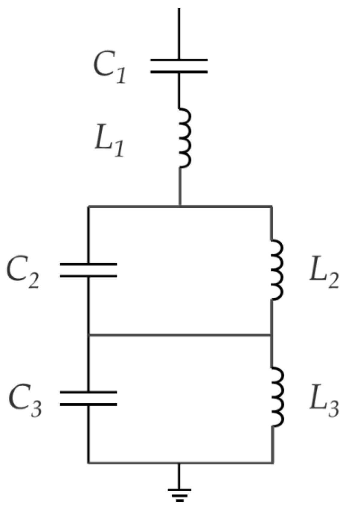
The direct triple-tuned filter (DTTF) mathematical model has never been presented in literature because of its complex mathematical formulations. The DTTF can be represented by adding an additional tuning circuit to the double-tuned filter, as shown in Figure 3.

For any angular frequency ω, the impedance of the series connection of the inductor and capacitor (L₁, C₁) is expressed as given in (27) while ignoring dielectric losses of capacitors and resistance in reactors. Its series resonance angular frequency (ω_s), which leads to a zero series impedance, i.e., Z_S = 0, can be written as follows:

$${\omega }_s=\frac{1}{\sqrt{L_1{C}_1}},$$

(27)

$$Z_s\left(\omega \right)=j\left(\omega L_1-\frac{1}{\omega C_1}\right).$$

(28)

Also, the impedances representing the two parallel connections of the inductors and capacitors (L₂, C₂) and (L₃, C₃) are expressed as given in (29) and (30) as Z_p1 and Z_p2, respectively.

$$Z_{p1}\left(\omega \right)=-j{\left(\omega C_2-\frac{1}{\omega L_2}\right)}^{-1},$$

(29)

$$Z_{p2}\left(\omega \right)=-j{\left(\omega C_3-\frac{1}{\omega L_3}\right)}^{-1}.$$

(30)

The parallel resonance angular frequencies (ω_p1 and ω_p2), which lead to infinite parallel impedances, i.e., Z_P = ∞, are given as:

$${\omega }_{p1}=\frac{1}{\sqrt{L_2{C}_2}},$$

(31)

$${\omega }_{p2}=\frac{1}{\sqrt{L_3{C}_3}}.$$

(32)

The parallel resonance frequencies can be expressed in terms of the fundamental frequency ω_f as follows:

$${\omega }_{p1}=m_{p1}{\omega }_f,$$

(33)

$${\omega }_{p2}=m_{p2}{\omega }_f.$$

(34)

where m_p1 and m_p2 are the parallel resonance harmonic orders.

Hence, the total impedance of the filter (Z_f) is expressed as:

$$Z_f\left(\omega \right)=Z_s\left(\omega \right)+Z_{p1}\left(\omega \right)+Z_{p2}\left(\omega \right)$$

(35)

Substituting (28)–(30) into (35) will lead to:

$$Z_f\left(\omega \right)=j\frac{({\omega }^2{L}_1{C}_1)({\omega }^2{L}_2{C}_2-1)({\omega }^2{L}_3{C}_3-1)-({\omega }^2{L}_2{C}_2-1)({\omega }^2{L}_3{C}_3-1)-({\omega }^2{L}_2{C}_1)({\omega }^2{L}_3{C}_3-1)-({\omega }^2{L}_3{C}_1)({\omega }^2{L}_2{C}_2-1)}{\omega C_1\left({\omega }^2{L}_2{C}_2-1\right)\left({\omega }^2{L}_3{C}_3-1\right)}$$

(36)

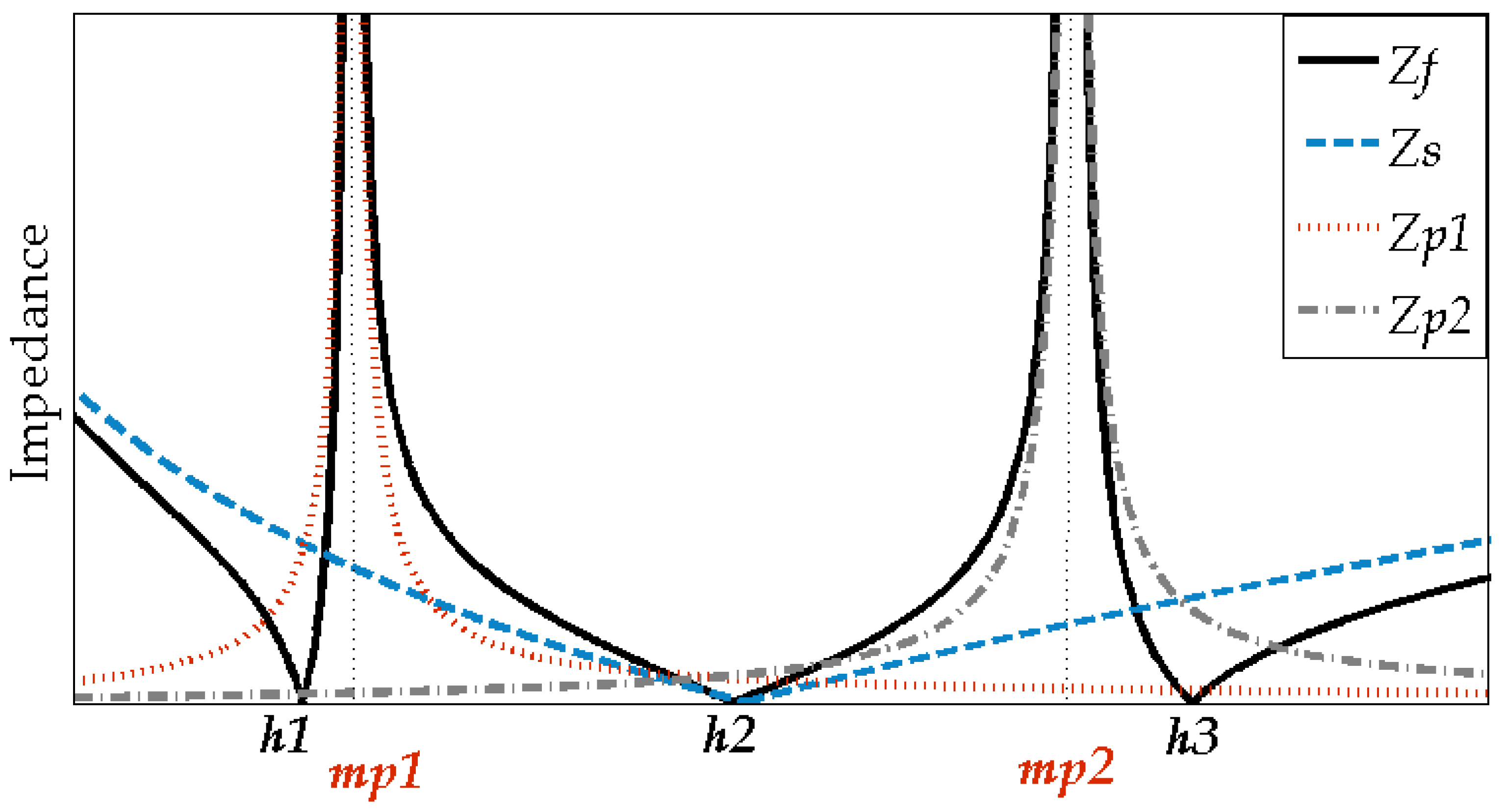
The series combination characteristic of the above three circuits (series and parallel) has three resonant frequencies (ω₁, ω_2, and ω₃), as shown in Figure 4. At the tuned frequencies, the total impedance of the filter is given as follows:

$$j\frac{({\omega }^2{L}_1{C}_1)({\omega }^2{L}_2{C}_2-1)({\omega }^2{L}_3{C}_3-1)-({\omega }^2{L}_2{C}_2-1)({\omega }^2{L}_3{C}_3-1)-({\omega }^2{L}_2{C}_1)({\omega }^2{L}_3{C}_3-1)-({\omega }^2{L}_3{C}_1)({\omega }^2{L}_2{C}_2-1)}{\omega C_1\left({\omega }^2{L}_2{C}_2-1\right)\left({\omega }^2{L}_3{C}_3-1\right)}=0$$

(37)

The numerator of (37) is given as:

$${\omega }^6{L}_1{L}_2{L}_3{C}_1{C}_2{C}_3-{\omega }^4\left(L_1{C}_1{L}_2{C}_2+L_1{C}_1{L}_3{C}_3+L_2{C}_2{L}_3{C}_3+L_2{C}_1{L}_3{C}_3+L_3{C}_1{L}_2{C}_2\right)+{\omega }^2\left(L_1{C}_1+L_2{C}_2+L_3{C}_3+L_2{C}_1+L_3{C}_1\right)-1=0$$

(38)

According to Vieta’s theory [15] and the theorem by A. Girard established for finding positive roots [16], the relationship between the three positive roots ω₁, ω₂, and ω₃ and the coefficients of (38) are given as follows:

$${{\omega }_1}^2{{\omega }_2}^2{{\omega }_3}^2=\frac{1}{L_1{C}_1{L}_2{C}_2{L}_3{C}_3}$$

(39)

From (28), (31), and (32), one can deduce that

$${\omega }_1{\omega }_2{\omega }_3={\omega }_s{\omega }_{p1}{\omega }_{p2}$$

(40)

The impedance resonance frequencies (ω₁, ω_2, and ω₃) can also be expressed in terms of the fundamental frequency as follows:

$${\omega }_1=h_1{\omega }_f,$$

(41)

$${\omega }_2=h_2{\omega }_f,$$

(42)

$${\omega }_3=h_3{\omega }_f.$$

(43)

where h₁, h_2, and h₃ are the harmonic tuning orders.

Further, by substituting (39) and (40) into (38):

$$\frac{{\omega }^6}{{\omega }_s^2{\omega }_{p1}^2{\omega }_{p2}^2}-{\omega }^4\left(\frac{1}{{\omega }_s^2{\omega }_{p1}^2}+\frac{1}{{\omega }_s^2{\omega }_{p2}^2}+\frac{1}{{\omega }_{p1}^2{\omega }_{p2}^2}\right)+{\omega }^2\left(\frac{1}{{\omega }_s^2}+\frac{1}{{\omega }_{p1}^2}+\frac{1}{{\omega }_{p2}^2}\right)-1=\frac{C_1}{C_2}\left(\frac{{\omega }^4}{{\omega }_{p1}^2{\omega }_{p2}^2}-\frac{{\omega }^2}{{\omega }_{p1}^2}\right)+\frac{C_1}{C_3}\left(\frac{{\omega }^4}{{\omega }_{p1}^2{\omega }_{p2}^2}-\frac{{\omega }^2}{{\omega }_{p2}^2}\right)$$

(44)

Then, assuming that the left-hand side of (44) equals A_w, therefore:

$$\frac{C_1}{C_2}\left(\frac{{\omega }^4}{{\omega }_{p1}^2{\omega }_{p2}^2}-\frac{{\omega }^2}{{\omega }_{p1}^2}\right)+\frac{C_1}{C_3}\left(\frac{{\omega }^4}{{\omega }_{p1}^2{\omega }_{p2}^2}-\frac{{\omega }^2}{{\omega }_{p2}^2}\right)=A_{\omega }$$

(45)

ω₁ is one of the solutions of (45), so at ω = ω₁, one can get:

$$\frac{C_1}{C_2}=A_{\omega 1}\frac{{\omega }_{p1}^2{\omega }_{p2}^2}{{\omega }_1^4-{\omega }_1^2{\omega }_{p2}^2}-\frac{C_1}{C_3}\left(\frac{{\omega }_1^4-{\omega }_1^2{\omega }_{p1}^2}{{\omega }_1^4-{\omega }_1^2{\omega }_{p2}^2}\right),$$

(46)

Also, ω₂ is one of the solutions of (45), so at ω = ω₂, one can get:

$$\frac{C_1}{C_3}=A_{\omega 2}\frac{{\omega }_{p1}^2{\omega }_{p2}^2}{{\omega }_2^4-{\omega }_2^2{\omega }_{p1}^2}-\frac{C_1}{C_2}\left(\frac{{\omega }_2^4-{\omega }_2^2{\omega }_{p2}^2}{{\omega }_2^4-{\omega }_2^2{\omega }_{p1}^2}\right).$$

(47)

Substituting (46) into (47), thus:

$$\frac{C_1}{C_3}=\left[A_{\omega 2}\frac{{\omega }_{p1}^2{\omega }_{p2}^2}{{\omega }_2^4-{\omega }_2^2{\omega }_{p1}^2}-A_{\omega 1}\frac{{\omega }_{p1}^2{\omega }_{p2}^2}{{\omega }_1^4-{\omega }_1^2{\omega }_{p2}^2}\left(\frac{{\omega }_2^4-{\omega }_2^2{\omega }_{p2}^2}{{\omega }_2^4-{\omega }_2^2{\omega }_{p1}^2}\right)\right]{\left[1-\left(\frac{{\omega }_1^4-{\omega }_1^2{\omega }_{p1}^2}{{\omega }_1^4-{\omega }_1^2{\omega }_{p2}^2}\right)\left(\frac{{\omega }_2^4-{\omega }_2^2{\omega }_{p2}^2}{{\omega }_2^4-{\omega }_2^2{\omega }_{p1}^2}\right)\right]}^{-1}$$

(48)

Then, assuming that the right-hand side of (48) equals B, hence:

$$C_3=\frac{C_1}{\mathrm{B}}$$

(49)

Substituting (49) into (45), thus:

$$C_2=\frac{C_1}{\left[A_{\omega 1}\left(\frac{{\omega }_{p1}^2{\omega }_{p2}^2}{{\omega }_1^4-{\omega }_1^2{\omega }_{p2}^2}\right)-\mathrm{B}\left(\frac{{\omega }_1^4-{\omega }_1^2{\omega }_{p1}^2}{{\omega }_1^4-{\omega }_1^2{\omega }_{p2}^2}\right)\right]}$$

(50)

At the fundamental frequency ω_f, and substituting by (49) and (50), (36) can be rewritten as follows:

$$Z\left({\omega }_f\right)=j\frac{\frac{{\omega }_f^6}{{\omega }_s^2{\omega }_{p1}^2{\omega }_{p2}^2}-{\omega }_f^4\left(\frac{1}{{\omega }_s^2{\omega }_{p1}^2}+\frac{1}{{\omega }_s^2{\omega }_{p2}^2}+\frac{1}{{\omega }_{p1}^2{\omega }_{p2}^2}\right)+{\omega }_f^2\left(\frac{1}{{\omega }_s^2}+\frac{1}{{\omega }_{p1}^2}+\frac{1}{{\omega }_{p2}^2}\right)-1-\frac{C_1}{C_2}\left(\frac{{\omega }_f^4}{{\omega }_{p1}^2-{\omega }_{p2}^2}-\frac{{\omega }_f^2}{{\omega }_{p1}^2}\right)-\frac{C_1}{C_3}\left(\frac{{\omega }_f^4}{{\omega }_{p1}^2-{\omega }_{p2}^2}-\frac{{\omega }_f^2}{{\omega }_{p2}^2}\right)}{{\omega }_f{C}_1\left(\frac{{\omega }_f^2}{{\omega }_{p1}^2}-1\right)\left(\frac{{\omega }_f^2}{{\omega }_{p2}^2}-1\right)}=-j\frac{V_s^2}{Q_f}$$

(51)

Substituting (44), (49), and (50) into (51), thus:

$$Z\left({\omega }_f\right)=\frac{A_{\omega f}-\left(A_{\omega 1}\left(\frac{{\omega }_{p1}^2{\omega }_{p2}^2}{{\omega }_1^4-{\omega }_1^2{\omega }_{p2}^2}\right)-\mathrm{B}\left(\frac{{\omega }_1^4-{\omega }_1^2{\omega }_{p1}^2}{{\omega }_1^4-{\omega }_1^2{\omega }_{p2}^2}\right)\right)\left(\frac{{\omega }_f^4}{{\omega }_{p1}^2-{\omega }_{p2}^2}-\frac{{\omega }_f^2}{{\omega }_{p1}^2}\right)-\mathrm{B}\left(\frac{{\omega }_f^4}{{\omega }_{p1}^2-{\omega }_{p2}^2}-\frac{{\omega }_f^2}{{\omega }_{p2}^2}\right)}{{\omega }_f{C}_1\left(\frac{{\omega }_f^2}{{\omega }_{p1}^2}-1\right)\left(\frac{{\omega }_f^2}{{\omega }_{p2}^2}-1\right)}=-\frac{V_s^2}{Q_f}$$

(52)

Finally, by simplifying (52), one can get the following expression for C₁:

$$C_1=\frac{A_{\omega f}-\left[A_{\omega 1}\frac{{\omega }_{p1}^2{\omega }_{p2}^2}{{\omega }_1^4-{\omega }_1^2{\omega }_{p2}^2}-\mathrm{B}\left(\frac{{\omega }_1^4-{\omega }_1^2{\omega }_{p1}^2}{{\omega }_1^4-{\omega }_1^2{\omega }_{p2}^2}\right)\right]\left[\frac{{{\omega }_f}^4}{{\omega }_{p1}^2{\omega }_{p2}^2}-\frac{{{\omega }_f}^2}{{\omega }_{p1}^2}\right]-\mathrm{B}\left(\frac{{{\omega }_f}^4}{{\omega }_{p1}^2{\omega }_{p2}^2}-\frac{{{\omega }_f}^2}{{\omega }_{p2}^2}\right)}{{\omega }_f\left(\frac{{{\omega }_f}^2}{{{\omega }_{p1}}^2}-1\right)\left(\frac{{{\omega }_f}^2}{{{\omega }_{p2}}^2}-1\right)}\frac{-Q_f}{V_s^2}$$

(53)

where,

$$A_{\omega f}=\frac{{\omega }_f^6}{{\omega }_s^2{\omega }_{p1}^2{\omega }_{p2}^2}-{\omega }_f^4\left(\frac{1}{{\omega }_s^2{\omega }_{p1}^2}+\frac{1}{{\omega }_s^2{\omega }_{p2}^2}+\frac{1}{{\omega }_{p1}^2{\omega }_{p2}^2}\right)+{\omega }_f^2\left(\frac{1}{{\omega }_s^2}+\frac{1}{{\omega }_{p1}^2}+\frac{1}{{\omega }_{p2}^2}\right)-1$$

(54)

Therefore, the filter capacitances can be calculated by (53), (50), and (49), and the inductances can be calculated as follows:

$$L_1=\frac{1}{{\omega }_s^2{C}_1},$$

(55)

$$L_2=\frac{1}{{\omega }_{P1}^2{C}_2},$$

(56)

$$L_3=\frac{1}{{\omega }_{P2}^2{C}_3}.$$

(57)

The design of DTTF is a complicated and complex mathematical analysis. However, its design equations have been solved, and its parameters can be optimized by selecting the proper harmonics orders to be eliminated, hence getting the values of capacitances and inductances.

2.3. Mathematical Design of Triple Tuned Filter Based on the Equivalence Hypothesis with TASTF

Another design of the TTF is proposed to obtain its parameters based on the equivalence hypothesis with TASTF. The equivalence hypothesis’s filter (EHF) can be found by equalizing the total impedance of both types. The TASTF total impedance (Z_f1) and the DTTF total impedance (Z_f2) can be written as:

$$Z_{f1}=j\left(\frac{{\omega }^6(L_a{C}_a{L}_b{C}_b{L}_c{C}_c)-{\omega }^4(L_a{C}_a{L}_b{C}_b+L_a{C}_a{L}_c{C}_c+L_b{C}_b{L}_c{C}_c)+{\omega }^2(L_a{C}_a+L_b{C}_b+L_c{C}_c)-1}{{\omega }^5(C_a{L}_b{C}_b{L}_c{C}_c+C_b{L}_a{C}_a{L}_c{C}_c+C_c{L}_a{C}_a{L}_b{C}_b)-{\omega }^3(C_a{L}_b{C}_b+C_a{L}_c{C}_c+C_b{L}_a{C}_a+C_b{L}_c{C}_c+C_c{L}_a{C}_a+C_c{L}_b{C}_b)+\omega (C_a+C_b+C_c)}\right),$$

(58)

$$Z_{f2}=j\left(\frac{{\omega }^6(L_1{C}_1{L}_2{C}_2{L}_3{C}_3)-{\omega }^4(L_1{C}_1{L}_2{C}_2+L_1{C}_1{L}_3{C}_3+L_2{C}_2{L}_3{C}_3+L_2{C}_1{L}_3{C}_3+L_3{C}_1{L}_2{C}_2)+{\omega }^2(L_1{C}_1+L_2{C}_2+L_3{C}_3+L_2{C}_1+L_3{C}_1)}{{\omega }^5(C_1{L}_2{C}_2{L}_3{C}_3)-{\omega }^3(C_1{L}_2{C}_2+C_1{L}_3{C}_3)+\omega C_1}\right).$$

(59)

As Z_f1 = Z_f2, analyzing and equalizing the coefficients of ω in both the numerator and denominator, one can get the following six equations:

$$C_1=C_a+C_b+C_c,$$

(60)

$$C_1{L}_2{C}_2+C_1{L}_3{C}_3=C_a{L}_b{C}_b+C_a{L}_c{C}_c+C_b{L}_a{C}_a+C_b{L}_c{C}_c+C_c{L}_a{C}_a+C_c{L}_b{C}_b,$$

(61)

$$C_1{L}_2{C}_2{L}_3{C}_3=C_a{L}_b{C}_b{L}_c{C}_c+C_b{L}_a{C}_a{L}_c{C}_c+C_c{L}_a{C}_a{L}_b{C}_b,$$

(62)

$$L_1{C}_1+L_2{C}_2+L_3{C}_3+L_2{C}_1+L_3{C}_1=L_a{C}_a+L_b{C}_b+L_c{C}_c,$$

(63)

$${\omega }^6{L}_1{L}_2{L}_3{C}_1{C}_2{C}_3-{\omega }^4\left(L_1{C}_1{L}_2{C}_2+L_1{C}_1{L}_3{C}_3+L_2{C}_2{L}_3{C}_3+L_2{C}_1{L}_3{C}_3+L_3{C}_1{L}_2{C}_2\right)+{\omega }^2\left(L_1{C}_1+L_2{C}_2+L_3{C}_3+L_2{C}_1+L_3{C}_1\right)-1=0,$$

(64)

$$L_1{C}_1{L}_2{C}_2{L}_3{C}_3=L_a{C}_a{L}_b{C}_b{L}_c{C}_c.$$

(65)

After complex mathematical analysis in solving these equations, the parameters of the TTF are given as follows:

$$C_1=C_a+C_b+C_c,$$

(66)

$$L_1=\frac{L_a{L}_b{L}_c}{L_a{L}_b+L_b{L}_c+L_a{L}_c},$$

(67)

$$C_2=\frac{Z_1(Z_3-Z_4)}{Z_2{Z}_3{Z}_4-Z_1{Z}_4},$$

(68)

$$L_2=\frac{Z_3(Z_3-Z_4)}{Z_1{Z}_3-Z_2{Z}_3{Z}_4},$$

(69)

$$C_3=\frac{Z_3(Z_3-Z_4)}{Z_1{Z}_3-Z_2{Z}_3{Z}_4},$$

(70)

$$L_3=\frac{Z_1{Z}_3-Z_2{Z}_3{Z}_4}{Z_3-Z_4}.$$

(71)

where

$$Z_1=\frac{C_a{L_a}^2{L}_b+C_b{L_b}^2{L}_c+C_c{L_c}^2{L}_a}{(C_a+C_b+C_c)X}-\frac{L_a{L}_b{L}_c}{X}-\frac{Y}{{(C_a+C_b+C_c)}^2},$$

(72)

$$Z_2=\frac{C_a{C}_b{L_a}^2{L_b}^2+C_a{C}_c{L_a}^2{L_c}^2+C_b{C}_c{L_b}^2{L_c}^2}{(C_a+C_b+C_c)X^2}-\frac{1}{C_a+C_b+C_c},$$

(73)

$$Z_3=\frac{Y}{2(C_a+C_b+C_c)}+{\left[{(\frac{Y}{2(C_a+C_b+C_c)})}^2-\frac{C_a{C}_b{C}_c}{C_a+C_b+C_c}X\right]}^{\frac{1}{2}},$$

(74)

$$Z_4=\frac{Y}{2(C_a+C_b+C_c)}-{\left[{(\frac{Y}{2(C_a+C_b+C_c)})}^2-\frac{C_a{C}_b{C}_c}{C_a+C_b+C_c}X\right]}^{\frac{1}{2}},$$

(75)

$$X=L_a{C}_a+L_b{C}_b+L_c{C}_c,$$

(76)

$$Y=C_a{L}_b{C}_b+C_a{L}_c{C}_c+C_b{L}_a{C}_a+C_b{L}_c{C}_c+C_c{L}_a{C}_a+C_c{L}_b{C}_b.$$

(77)

The relationship between the resonance frequency of the two filters is then represented as follows:

$${\omega }_{ra}{\omega }_{rb}{\omega }_{rc}={\omega }_s{\omega }_{p1}{\omega }_{p2}$$

(78)

3. System Studied

3.1. System Description and Problem Formulation

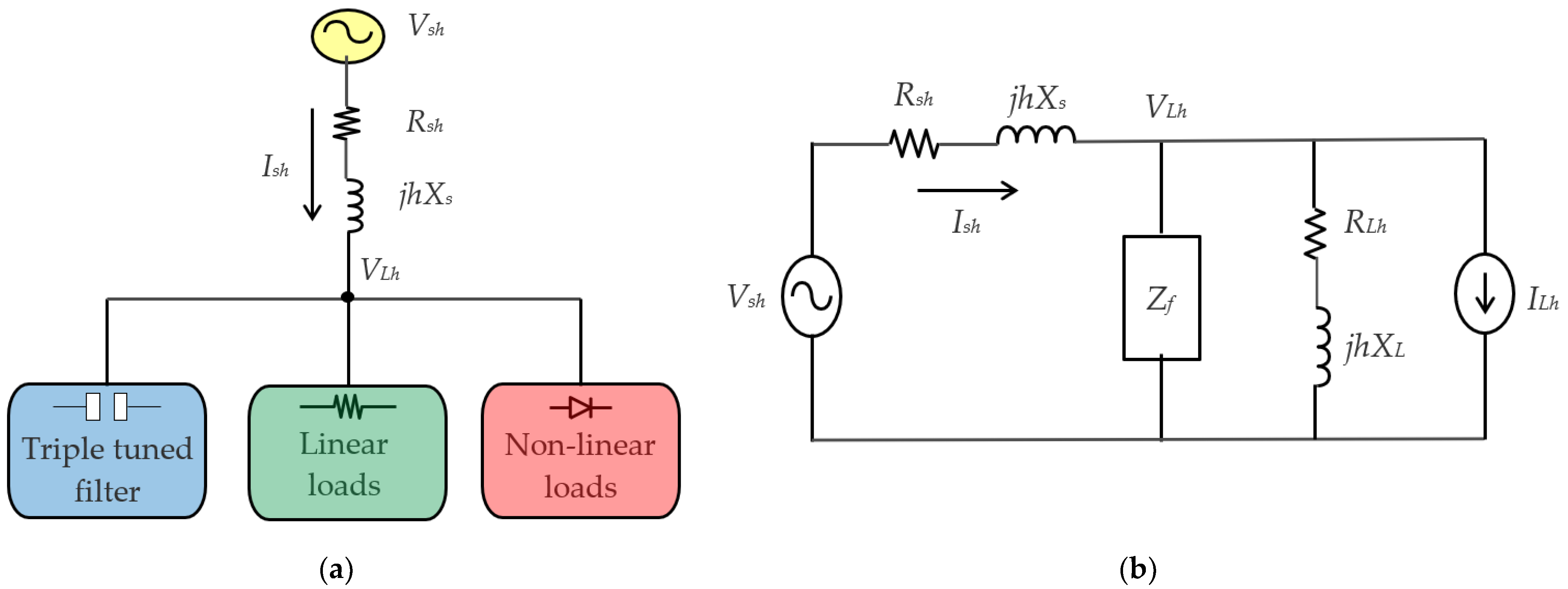
The studied system comprises a utility system, mixed linear and nonlinear loads, and filters. The single-line diagram of the system under study is shown in Figure 5a. Its equivalent circuit representing the utility with Thevenin’s voltage source and Thevenin resistance is illustrated in Figure 5b, where R_s and X_s represent the fundamental resistance and reactance of the line impedance at harmonic order h, and the linear load is modeled as a resistance R_L connected in series with inductance X_L in ohms at h. The filter is modeled as a resistance R_F connected in series with inductance X_F in ohms at the harmonic order h.

In the equivalent circuit, the impedance of the linear load, supply line, and filter are expressed as the hth harmonic impedances denoted $Z_{Sh}$, $Z_{Lh}$ and $Z_{Fh}$, respectively, thus:

$$Z_{Sh}=R_S+jh{X}_S,$$

(79)

$$Z_{Lh}=R_L+jh{X}_L,$$

(80)

$$Z_{Fh}=R_F+jh{X}_F.$$

(81)

Based on the circuit theorems, at the hth harmonic order, expressions of the line current $I_{sh}$ and load bus voltage $V_{Lh}$ can be expressed as follows:

$$I_{sh}=\frac{V_{Sh}}{Z_{Sh}+Z_{FLh}}+\frac{Z_{FLh}}{Z_{Sh}+Z_{FLh}}{I}_{Lh},$$

(82)

$$V_{Lh}=V_{Sh}-I_{Sh}{Z}_{Sh}$$

(83)

where $Z_{FLh}$ represents the parallel equivalent impedance of the filter’s impedance $Z_{Fh}$ and the load impedance $Z_{Lh}.$; so that

$$Z_{FLh}=\frac{Z_{Fh}{Z}_{Lh}}{Z_{Fh}+Z_{Lh}}$$

(84)

The per-phase transmission line power losses $\Delta P_L$ can be expressed as follows:

$$\Delta P_L={\displaystyle \sum _{h\ge 1}{I}_{Sh}^2{R}_S}$$

(85)

Total harmonic distortion voltage THD_V is used to specify the effective voltage value of the harmonic orders injected in the power system at the fundamental voltage and can be calculated as follows:

$$THDV(\%)=\frac{\sqrt{{\displaystyle {\sum }_{h\ne 1}{V}_h^2}}}{V_1}\times 100,$$

(86)

Total harmonic distortion current THD_I and the total demand distortion TDD_I are used to specify the effective current value of the harmonic orders injected in the power system relative to the fundamental current and can be expressed as:

$$THDI(\%)=\frac{\sqrt{{\displaystyle {\sum }_{h\ne 1}{I}_h^2}}}{I_1}\times 100,$$

(87)

$$TDDI(\%)=\frac{\sqrt{{\displaystyle {\sum }_{h\ne 1}{I}_h^2}}}{I_L}\times 100$$

(88)

where $V_1$ denotes the fundamental component of the load voltage, $I_1.$ denotes the fundamental component of the source current, and I_L denotes the maximum load demand.

3.2. Objective Function Formulation

According to [17], the adaptive weighted sum technique successfully solves issues with multiple objectives. Hence, in order to ensure enhancement of the power quality of the system using different performance terms, a multi-objective function is used to minimize the transmission line power losses given in (85) and the total voltage and current harmonic distortion given in (86) and (87). The objective function can be expressed as:

$$F=\mathrm{Minimize} [k_1\times \Delta P_L+k_2\times TH{D}_V+k_3\times TH{D}_I]$$

(89)

where $k_1$, $k_2$ and $k_3$ are the adaptive weights used in minimizing the power losses, THD_V and THD_I respectively, where $k_1\ge 0$, $k_2\ge 0$, $k_3\ge 0$ and $k_1+k_2+k_3=1$. Hence, the optimal filter design can be determined by choosing the optimal values for Q_f, h_a, h_b, h_c, mp₁, mp₂ for the TASTF and Q_f, h₁, h₂, h₃, mp₁, mp₂ for the DTTF.

3.3. Constraints

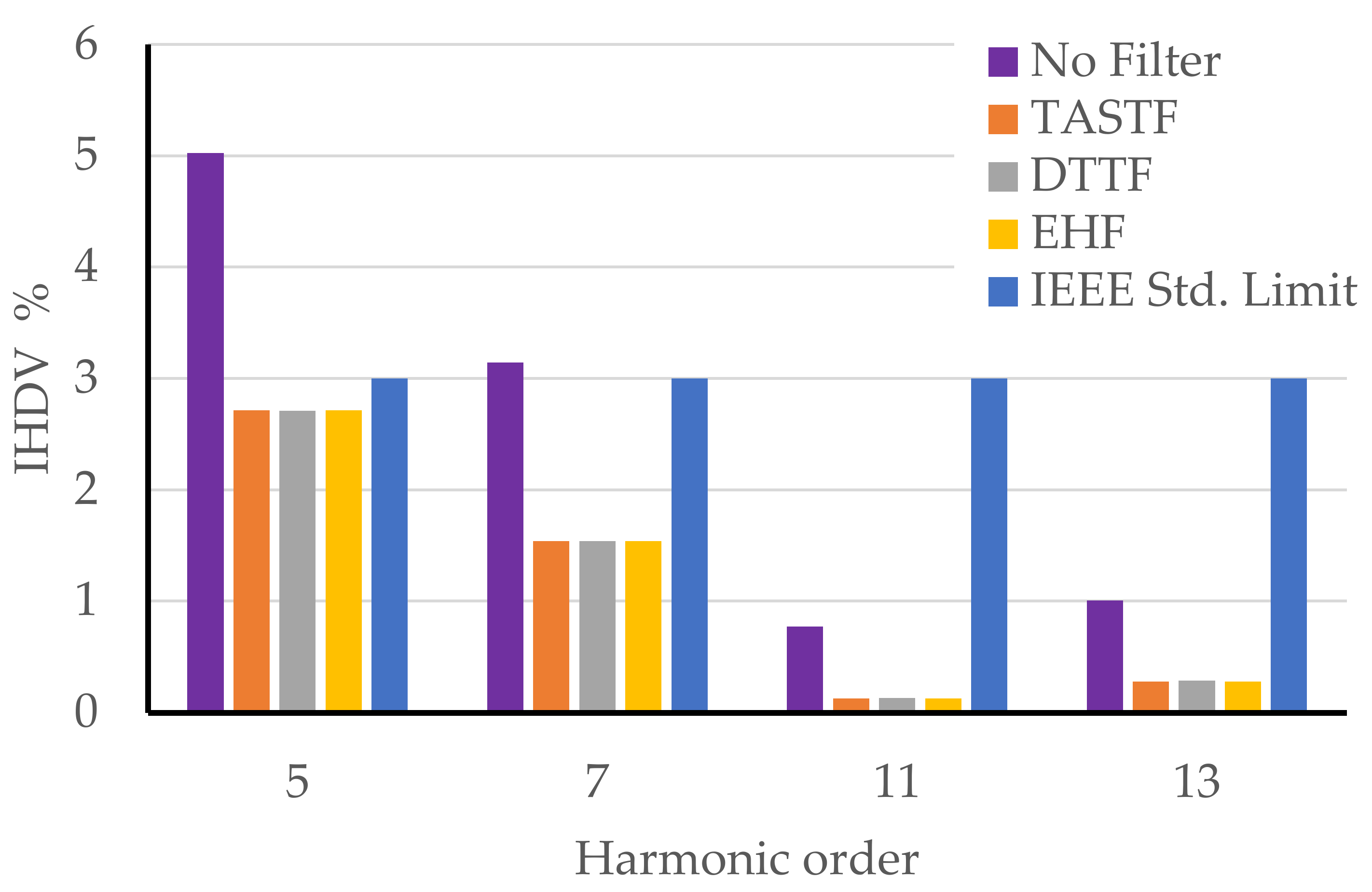
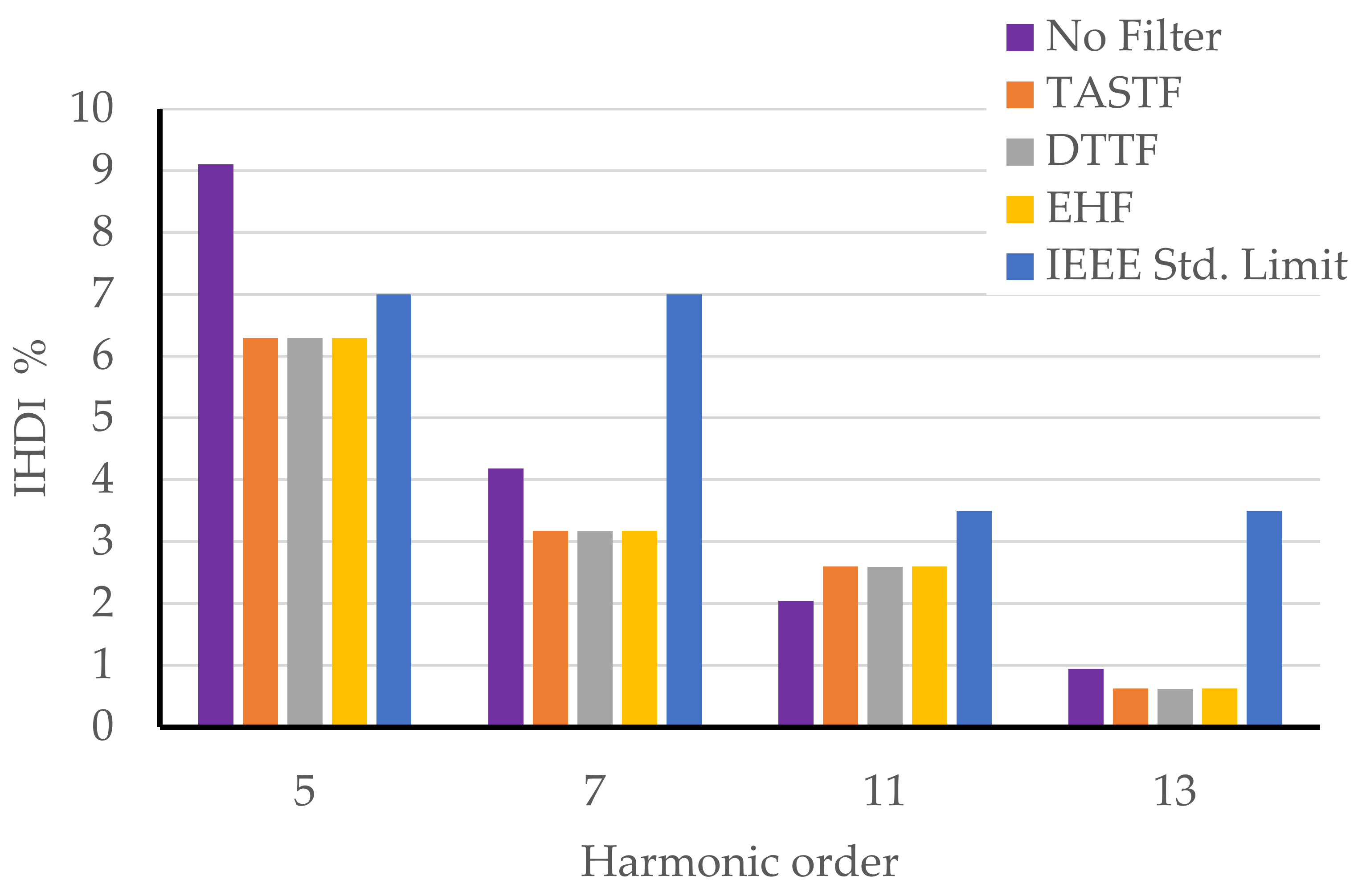
As reported in IEEE Std. 519 [18] and the Egyptian practice codes, preserving the displacement power factor (DPF) in an acceptable range higher than 90% lagging is desirable (90%≤ DPF ≤ 100%). The total demand distortion current (TDD_I) should be in an acceptable range below 8%, i.e., TDD_I ≤ 8%, and the individual current harmonic orders must be below 7 % for the 5th and 7th harmonic orders and 3.5% for the 11th and 13th harmonic orders. The total harmonic distortion voltage (THD_V) should be in a satisfactory range (THD_V ≤ 5%). Also, all individual voltage harmonic distortion must be limited to less than or equal to 3%.

4. Optimization Techniques

This paper uses a novel optimization called artificial rabbits optimization to optimize the filter parameters based on the TASTF, DTTF, and EHF design methods. In order to get the best solutions, the ant lion algorithm and whale optimizer algorithm are used to validate the results obtained.

4.1. Artificial Rabbits Optimization

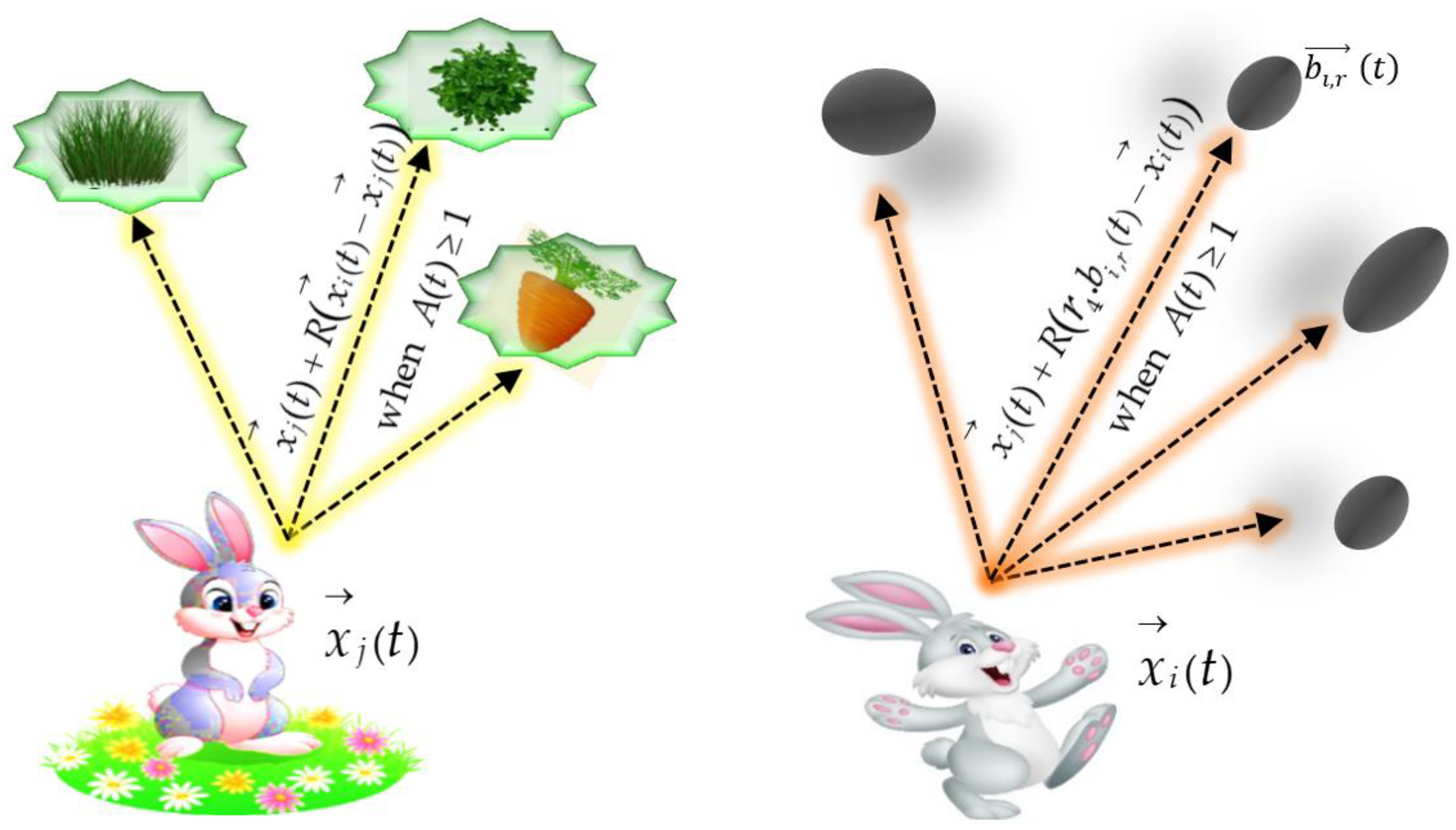
Artificial rabbits optimization (ARO), a new bio-inspired meta-heuristic method, was proposed and thoroughly tested by Wang et al. in 2022 for solving engineering problems. ARO was inspired by how rabbits in the wild survive. As herbivores, rabbits mostly eat grass, forbs, and leafy weeds. Rabbits never consume the grass close to their holes; instead, they seek nourishment elsewhere to avoid predators discovering their nest. Random hiding is another means of rabbit survival. Rabbits must move quickly to avoid their many predators because they are at the bottom of the food chain, which will shrink their energy, so rabbits need to adaptively switch between detour foraging and random hiding [19].

Rabbits search far and disregard what is nearby when foraging. That is called the foraging habit “detour foraging” since they only consume grass randomly in other places. The following expression represents the mathematical model of rabbits’ detour foraging [19]:

$$\begin{array}{l}\overrightarrow{v_i}(t+1)={\overrightarrow{x}}_j(t)+R({\overrightarrow{x}}_i(t)-{\overrightarrow{x}}_j(t))+round(0.5(0.05+r_1))n_1,\\ i,j=1,\dots \dots ,nandj\ne i\end{array}$$

(90)

$$R=LC$$

(91)

where n is the size of the population, $\overrightarrow{v_i}\left(t+1\right)$ is the candidate position of the ith rabbit at the time t + 1, $\overrightarrow{x_i}\left(t\right), \overrightarrow{x_j}\left(t\right)$ denotes the locations of the ith or jth rabbit at the time t, rand returns a random permutation of integers from 1 to the dimension of the problem (d), r₁ is a random number between 0 and 1, L is the running length, which represents the movement speed when carrying out the detour foraging, C is 0 or 1, and n₁ subjects to the standard normal distribution. Predators frequently pursue and attack rabbits. Rabbits must locate a secure hiding spot if they are to live. In order to avoid being discovered, they are forbidden from choosing a burrow at random for refuge. The following equations mathematically describe this random concealment technique [19]:

$$\begin{array}{l}\overrightarrow{v_i}(t+1)={\overrightarrow{x}}_j(t)+R(r_4.b_{i,r}(t)-{\overrightarrow{x}}_i(t))\hspace{1em},i=1,\dots \dots ,n\\ \end{array}$$

(92)

where $\overrightarrow{b_{j,r}} \left(t\right)$ represents a randomly selected burrow for hiding from its d burrows, and r₄ denotes a random number between 0 and 1. The energy of a rabbit, which will progressively diminish over time, powers the search mechanism. In order to represent the transition from exploration to exploitation, an energy component is created. The following is a definition of the energy factor in ARO [19]:

$$A(t)=4(1-\frac{t}{T})\ln \frac{1}{r}$$

(93)

where $A\left(t\right)$ denotes the energy factor, r is the random number between 0 and 1, and T is the maximum number of iterations.

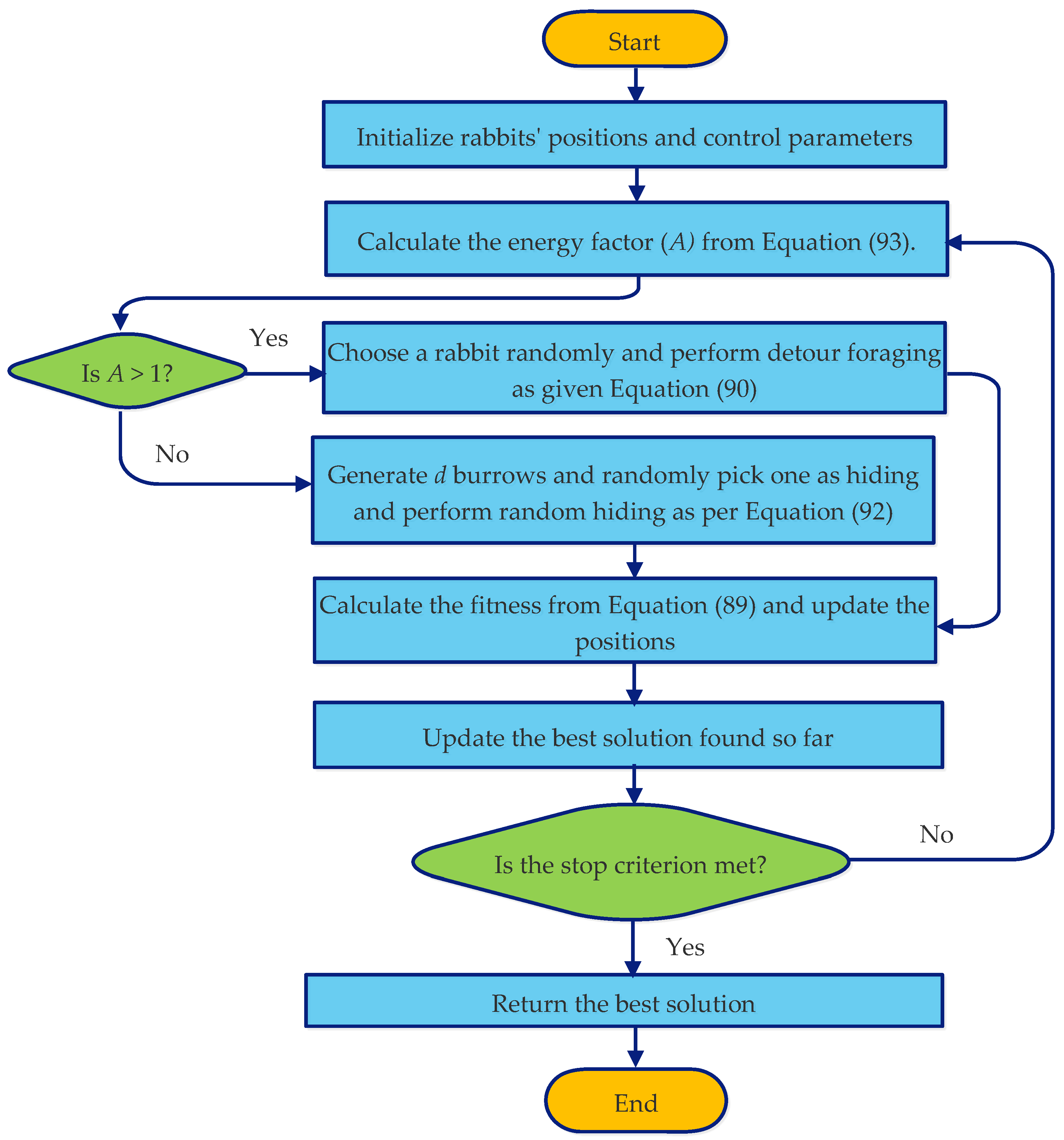
The search mechanism is depicted in Figure 6, which illustrates that the ARO algorithm creates a collection of random populations of artificial rabbits (possible solutions) in the search space. A rabbit updates its location concerning either a randomly selected rabbit from the population or a randomly chosen rabbit from one of its burrows at each iteration. By increasing the number of iterations, the energy factor A decreases, which might drive every member of the population to alternate between detour foraging activity and random hiding behavior. The best-so-far answer is returned once all updating and computation have been completed interactively and the termination requirement has been fulfilled. Figure 7 explores the flowchart of the ARO algorithm.

4.2. Ant Lion Optimizer

Mirjalili presented a nature-inspired algorithm called ant lion optimizer (ALO) in 2015 [20]. The ALO algorithm imitates the way ant lions hunt in nature. There are five basic processes in hunting prey: setting up traps, entrapping ants in them, capturing prey, and setting up new traps. An insect belonging to the net-winged, or Neuroptera, order is called an ant lion. More detail about ALO can be found in [20].

4.3. Whale Optimization Algorithm

In 2016, Mirjalili and Lewis introduced the whale optimization algorithm (WOA) to metaheuristic algorithms [21]. The distinctive way humpback whales hunt inspired the authors of [21] to develop the WOA. The WOA mathematical model is described in detail in [21].

5. Results and Discussion

This section presents the results obtained from the TASTF, DTTF, and EHF. All proposed algorithms are developed using MATLAB™. The system parameters investigated in this study are obtained from an illustrative example presented in IEEE Std. 519 [18]. These parameters are shown in

Table 1. System data.

Parameter	Value
Line voltage of the AC network (kV)	4.16
Frequency (Hz)	50
Three-phase short circuit capacity (MVA)	150
Three-phase fundamental frequency active power (MW)	5.1
Three phases fundamental frequency reactive power (MVAr)	4.965
Thevenin’s resistance (Ω)	0.0115
Thevenin’s reactance (Ω)	0.1154
Resistance of the linear load impedance (Ω)	1.742
Reactance of the linear load impedance (Ω)	1.696
Transmission line power losses per phase (kW)	31.7406
VS5 (%)	5.023
VS7 (%)	3.144
VS11 (%)	0.772
VS13 (%)	1.008
IL5 (%)	9.098
IL7 (%)	4.184
IL11 (%)	2.04
IL13 (%)	0.938

.

The search populations for all optimization techniques were set to 50, and the maximum number of iterations was 100. The lower and upper bounds for Q_f, h₁, h₂, h₃, mp_1, and mp₂ are given in

Table 2. The parameters’ search space.

Parameter	Qf (kVAr)	h1	h2	h3	mp1	mp2
Lower bound	0	4	6	9.8	5	7
Upper bound	2000	4.9	6.9	12.5	5.9	9.5

. The adaptive weights k₁, k_2, and k₃ were chosen after many trials as 0.5, 0.25, and 0.25, respectively.

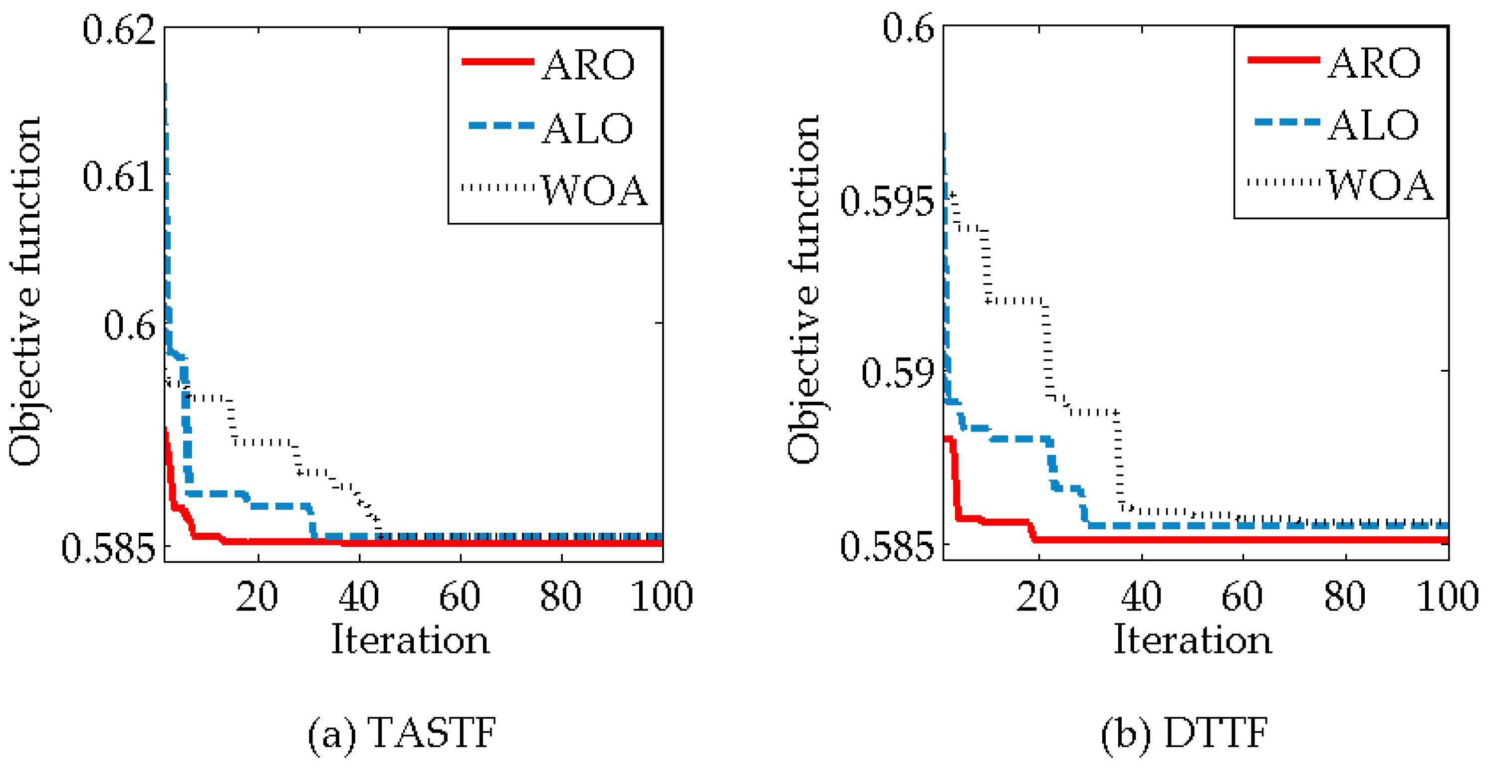
The ARO, ALO, and WOA techniques have shown their ability to enhance the system power quality, and the results are almost nearby. However, the ARO shows its superiority in finding the optimal parameters by selecting a minimum filter reactive power in a lower execution time with a slight reduction of power losses and voltage THD than ALO and WOA, as presented in

Table 3. Results obtained by the optimization algorithms.

Parameter	TASTF			DTTF
	ARO	ALO	WOA	ARO	ALO	WOA
Qf (kVAr)	1617.8230	1626.8774	1630.2466	1617.7685	1624.2584	1632.0160
Ploss (kW)	17.2833	17.2858	17.2873	17.2833	17.2844	17.2872
THDv (%)	3.1330	3.1356	3.1362	3.1341	3.1528	3.1544
TDDI (%)	5.3723	5.4532	5.4702	5.3726	5.4622	5.4683
Execution time (s)	14.7600	17.4820	19.0370	14.8950	18.0020	19.5370

. This is also presented in Figure 8, which shows the convergence curves of the ARO, ALO, and WOA for optimizing the TASTF and DTTF parameters. It illustrates that ARO converges to the minimum fitness value after 20 iterations. Thus, the optimized values obtained by ARO are used in the different investigations presented in the paper.

The optimized values of the TASTF and DTTF obtained with ARO and those calculated for EHF are explored in

Table 4. Optimized values of the TASTF and DTTF obtained with ARO.

Parameter	TASTF	DTTF	EHF
Qf (kVAr)	1617.8230	1617.7685	1617.8923
h1	4.5483	4.5180	4.5481
h2	6.0600	6.0726	6.0601
h3	10.0000	10.0001	10.0000
mp1	5.2444	5.2665	5.2443
mp2	7.8443	7.8710	7.8442
C1 (mF)	0.4100	0.8622	0.8631
L1 (mH)	1.1947	0.2683	0.2615
C2 (mF)	0.2378	7.4087	7.9553
L2 (mH)	1.1602	0.0493	0.0463
C3 (mF)	0.2153	2.0201	2.0812
L3 (mH)	0.4706	0.0810	0.0791

, indicating that the three methods’ parameters are almost close.

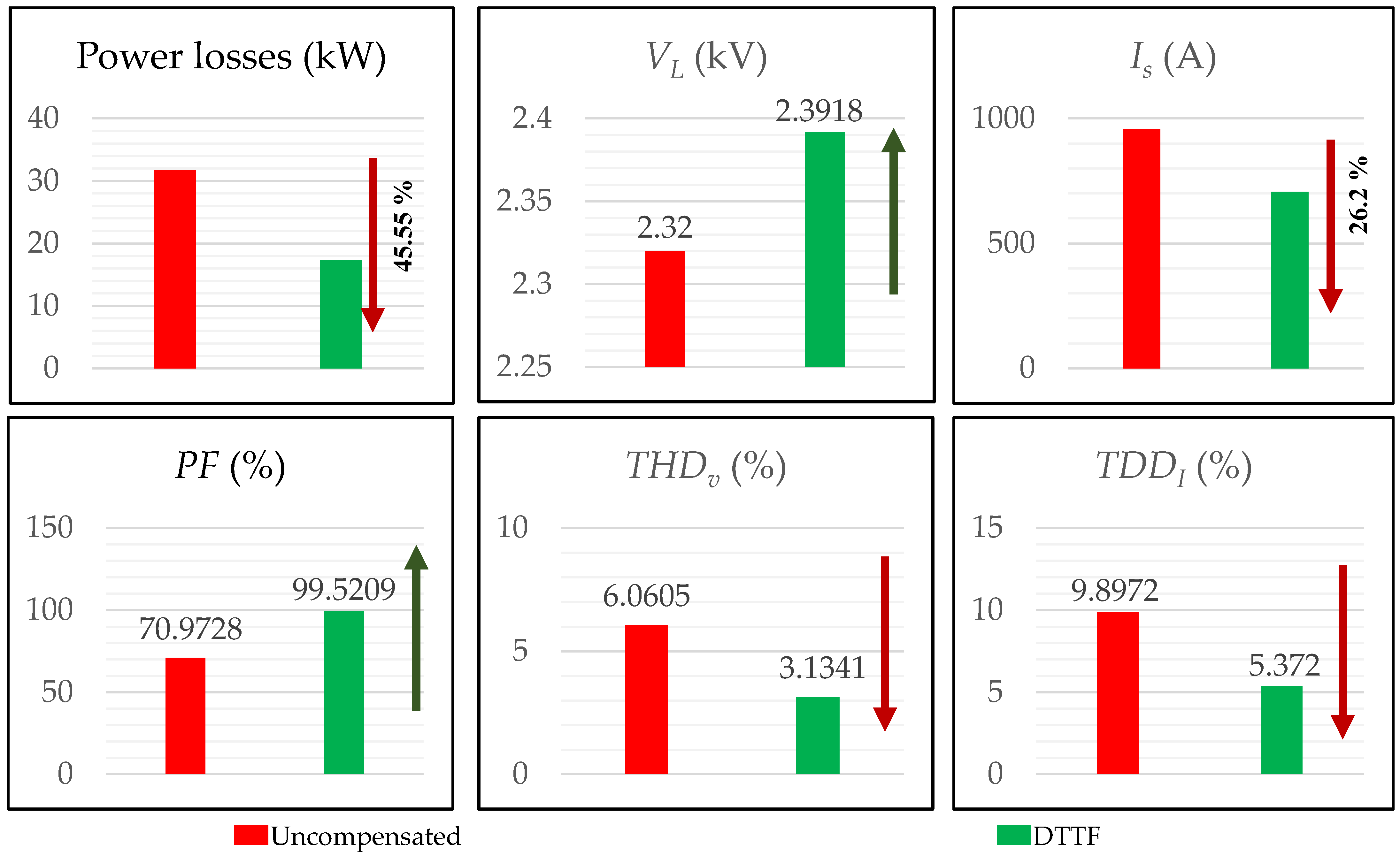
In order to evaluate the effectiveness of the proposed design methodologies of the proposed filter, the results obtained using ARO are compared with the results presented in the comparative analysis of the double-tuned harmonic passive filter design methodologies in [8], multi-arm single-tuned (MAST), direct design method (DDM) and analogy method (AM) between them. The comparison in

Table 5. Compensated system results compared to the original system and the results in [8].

Parameter	Uncompensated	Triple Tuned			Double Tuned [8]
		TASTF	DTTF	EHF	MAST	DDM	AM
Qf (kVAr)	---------	1617.8230	1617.7685	1617.8923	1849.5500	1663.6244	1660.5176
Ploss (kW)	31.7406	17.2833	17.2833	17.2833	17.3994	17.3995	17.3993
PF	70.9728	99.5210	99.5209	99.5211	98.9021	98.2548	99.4870
DPF	71.6527	99.9761	99.9760	99.9762	99.3515	98.7322	99.9487
THDv	6.0605	3.1330	3.1341	3.1340	3.4236	3.1129	3.5758
THDI	10.2629	7.5330	7.5310	7.5313	7.1631	7.7262	7.1833
TDDI	9.8972	5.3724	5.3720	5.3700	5.1027	5.4872	5.0614
VL (kV)	2.3200	2.3917	2.3918	2.3917	2.4029	2.3805	2.3912
Is	957.6339	706.6515	706.6502	706.6510	714.1830	712.3240	706.4221

validates the presented optimal designs’ effectiveness with ARO in minimizing the total power losses and enhancing the system power quality indices with a much lower filter rating. The results also confirmed that the three proposed methods have almost the same impact on the system’s performance. The DTTF positively impacts the system power quality levels, as shown in Figure 9. It was found that the power losses decreased by 45.55%, THD_V decreased to 3.1341%, TDD_I decreased to 5.372%, and the power factor (PF) increased to 99.5209%, which significantly enhanced the load bus voltage, which increased to 2.3918 kV, reduced the line current by 26.2%, while complying with all constraints.

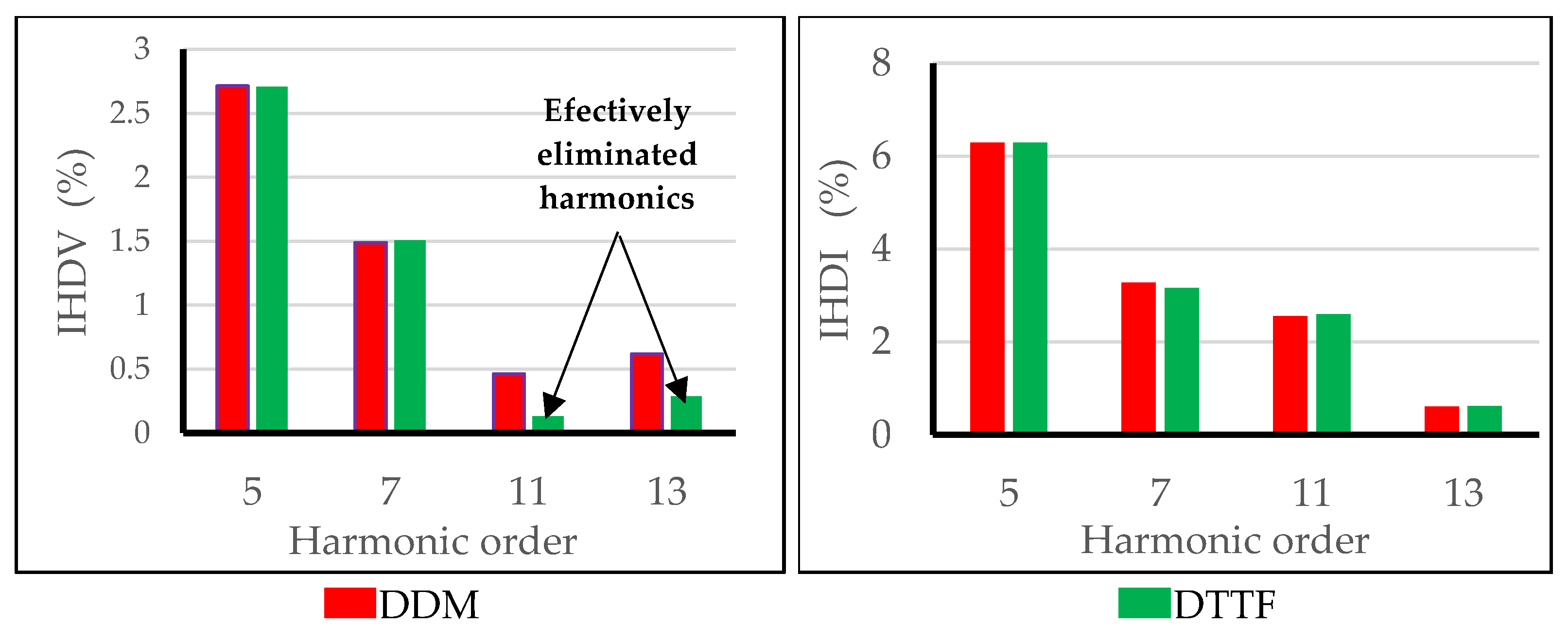
Figure 10 and Figure 11 show the individual harmonic distortion of load voltage (IHD_V) and source current (IHD_I) and their maximum values reported in IEEE Std. 519 [18]. Figure 12 shows IHD_V and IHD_I after compensation when using the DTTF compared to that obtained using the DDM [8]. It was found that using the DTTF can reduce the voltage harmonic distortion of the 11th and 13th orders more than the DDM without any adverse effects on their current harmonic distortion. In addition to the benefits of the TTF shown, it can eliminate a wide range of harmonic orders by adjusting the tuned harmonic orders as required in highly harmonically-polluted systems.

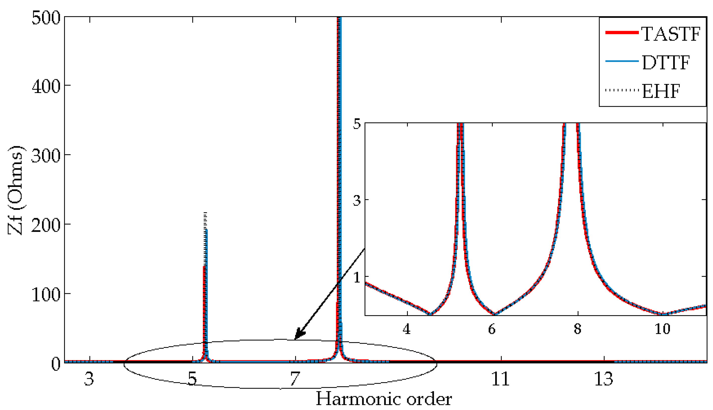
The total filter impedances for the TASTF, DTTF, and EHF are explored in Figure 13, which shows that the three impedances are almost identical. That indicates the superiority of the combination of mathematical and optimization formulation for the three filters to obtain the optimal values of the parameters needed for power quality enhancement.

6. Conclusions

A new mathematical model for the triple-tuned filter is thoroughly presented in three different design approaches—TASTF, DTTF, and EHF. The TASTF mathematical design is simple, unlike the DTTF, which was found to be complicated and provides the filter design in one shot. On the other side, the EHF’s mathematical analysis was complex and relied on designing the TASTF. The provided designs are then optimized to mitigate the system harmonics, minimize the power losses, and enhance power quality using a candidate-weighted multi-objective function for minimizing voltage THD, current THD, and power losses. The optimization techniques ARO, ALO, and WOA, are utilized to get the optimal filter parameters.

The system presented in IEEE STD-519-1992 is investigated in this study. The results obtained validate the efficiency of the ARO-based design to enhance the system power quality (it converged to the minimum fitness value after 20 iterations while utilizing lower filter reactive power). The power losses were reduced by 45.55%, THD_v was reduced to 3.134% instead of 6.061%, TDD_I was decreased to 5.37% instead of 9.897%, and the power factor was enhanced to reach 99.5209%. There was also a significant impact on reducing the line current by 26.2% and improving the load bus voltage, which increased to 2.392 kV. The in-depth comparative analysis of the simulation results highlights how well the three proposed designs enhance the system using less reactive power, making them much more economical in industrial and commercial applications.

Finally, the design strategy confirmed the ability to provide and optimize the triple-tuned filter that will enable researchers to design quad-tuned filters and others. Future works will investigate the damped filter design and its practical implementation and economic benefits.

References

- Lumbreras, D.; Gálvez, E.; Collado, A.; Zaragoza, J. Trends in power quality, harmonic mitigation and standards for light and heavy industries: A review. Energies 2020, 13, 5792. [Google Scholar] [CrossRef]
- Electric, S. Electrical Installation Guide According to IEC International Standards; Zobaa, A.F., Aleem, S.H.E.A., Abdelaziz, A.Y., Eds.; Classical and Recent Aspects of Power System Optimization; Academic Press: Cambridge, MA, USA; Elsevier: Amsterdam, The Netherlands, 2018; ISBN 9780128124413. [Google Scholar]
- Khattab, N.M.; Abdel Aleem, S.H.E.; El’Gharably, A.F.; Boghdady, T.A.; Turky, R.A.; Ali, Z.M.; Sayed, M.M. A novel design of fourth-order harmonic passive filters for total demand distortion minimization using crow spiral-based search algorithm. Ain Shams Eng. J. 2022, 13, 101632. [Google Scholar] [CrossRef]
- Fahmy, M.A.; Ibrahim, A.M.; Baici, M.E.; Aleem, S.H.E.A. Multi-objective optimization of double-tuned filters in distribution power systems using Non-Dominated Sorting Genetic Algorithm-II. In Proceedings of the 2017 10th International Conference on Electrical and Electronics Engineering, ELECO 2017, Bursa, Turkey, 30 November–2 December 2017; Elsevier: Amsterdam, The Netherlands; pp. 195–200, ISBN 9786050107371. [Google Scholar]
- Cheepati, K.R.; Ali, S.; Suraya Kalavathi, M. Overview of double tuned harmonic filters in improving power quality under non linear load conditions. Int. J. Grid Distrib. Comput. 2017, 10, 11–26. [Google Scholar] [CrossRef]
- Kahar, N.H.B.A.; Zobaa, A.F. Optimal single tuned damped filter for mitigating harmonics using MIDACO. In Proceedings of the 2017 IEEE International Conference on Environment and Electrical Engineering and 2017 IEEE Industrial and Commercial Power Systems Europe (EEEIC/I&CPS Europe), Milan, Italy, 6–9 June 2017; pp. 17–20. [Google Scholar] [CrossRef]
- Melo, I.D.; Pereira, J.L.R.; Variz, A.M.; Ribeiro, P.F. Allocation and sizing of single tuned passive filters in three-phase distribution systems for power quality improvement. Electr. Power Syst. Res. 2020, 180, 106128. [Google Scholar] [CrossRef]
- Zobaa, A.M.; Abdel Aleem, S.H.E.; Youssef, H.K.M. Comparative Analysis of Double-Tuned Harmonic Passive Filter Design Methodologies Using Slime Mould Optimization Algorithm. In Proceedings of the 2021 IEEE Texas Power and Energy Conference (TPEC), College Station, TX, USA, 2–5 February 2021. [Google Scholar] [CrossRef]
- Bartzsch, C.; Huang, H.; Roessel, R.; Sadek, K. Triple tuned harmonic filters-design principle and operating experience. In Proceedings of the International Conference on Power System Technology, Kunming, China, 13–17 October 2002; Volume 1, pp. 542–546. [Google Scholar] [CrossRef]
- Bo, C.; Xiangjun, Z.; Yao, X. Three tuned passive filter to improve power quality. In Proceedings of the 2006 International Conference on Power System Technology, Chongqing, China, 22–26 October 2006. [Google Scholar] [CrossRef]
- Li, P.; Hao, Q. The algorithm for the parameters of AC filters in HVDC transmission system. In Proceedings of the 2008 IEEE/PES Transmission and Distribution Conference and Exposition, Chicago, IL, USA, 21–24 April 2008. [Google Scholar] [CrossRef]
- Klempka, R. Design and optimisation of a simple filter group for reactive power distribution. Math. Probl. Eng. 2016, 2016, 4125014. [Google Scholar] [CrossRef] [Green Version]
- Karadeniz, A.; Balci, M.E. Comparative evaluation of common passive filter types regarding maximization of transformer’s loading capability under non-sinusoidal conditions. Electr. Power Syst. Res. 2018, 158, 324–334. [Google Scholar] [CrossRef]
- Klempka, R. Analytical optimization of the filtration efficiency of a group of single branch filters. Electr. Power Syst. Res. 2022, 202, 107603. [Google Scholar] [CrossRef]
- Viète, F. Opera Mathematica; van, F., Schooten, Ed.; Lvgdvni Batavorvm, ex officinâ Bonaventuræ & Abrahami Elzeviriorum. 1646. Available online: https://www.loc.gov/item/26006234/ (accessed on 16 November 2022).
- Girard, A. Invention nouvelle en l’algèbre. Haan, e.D.B.d., Ed.; Imprimé chez Muré frères: Leiden, Holland, 1884. [Google Scholar]
- Maher, M.; Ebrahim, M.A.; Mohamed, E.A.; Mohamed, A. Ant-lion inspired algorithm based optimal design of electric distribution networks. In Proceedings of the 2017 Nineteenth International Middle East Power Systems Conference (MEPCON), Cairo, Egypt, 19–21 December 2017; pp. 613–618. [Google Scholar] [CrossRef]
- IEEE Standard 519-1992; IEEE Recommended Practice and Requirements for Harmonic Control in Electric Power Systems. IEEE: New York, NY, USA, 2014.
- Wang, L.; Cao, Q.; Zhang, Z.; Mirjalili, S.; Zhao, W. Artificial rabbits optimization: A new bio-inspired meta-heuristic algorithm for solving engineering optimization problems. Eng. Appl. Artif. Intell. 2022, 114, 105082. [Google Scholar] [CrossRef]
- Mirjalili, S. The ant lion optimizer. Adv. Eng. Softw. 2015, 83, 80–98. [Google Scholar] [CrossRef]
- Mirjalili, S.; Lewis, A. The Whale Optimization Algorithm. Adv. Eng. Softw. 2016, 95, 51–67. [Google Scholar] [CrossRef]
Figure 1.
The three arms of a single-tuned filter.
Figure 2.
Impedance characteristic of the TASTF.
Figure 3.
The direct triple-tuned filter.
Figure 4.
DTTF’s impedance characteristic.
Figure 5.
The system under study: (a) Its single line diagram; (b) Its per-phase equivalent circuit.
Figure 6.
Search mechanism based on the energy factor.
Figure 7.
ARO algorithm’s flowchart.
Figure 8.
ARO, ALO, and WOA’s convergence curves.
Figure 9.
Performance of the DTTF in terms of the investigated metrics.
Figure 10.
The individual load voltage harmonics.
Figure 11.
The individual load current harmonics.
Figure 12.
The system’s individual load voltage and current harmonics using DTTF compared with DDM in [8].
Figure 13.
The filter impedance of TASTF, DTTF, and EHF.