Article

A Neuro-Predictive Controller Scheme for Integration of a Basic Wind Energy Generation Unit with an Electrical Power System

by
Mohamed Abd-El-Hakeem Mohamed
1,
Hossam Seddik Abbas
2,
Mokhtar Shouran
3,* and
Salah Kamel
4
1
Faculty of Engineering, Al-Azhar University, Qena 83511, Egypt
2
Faculty of Engineering, Assuit University, Assuit 71543, Egypt
3
Wolfson Centre for Magnetics, School of Engineering, Cardiff University, Cardiff CF24 3AA, UK
4
Electrical Engineering Department, Faculty of Engineering, Aswan University, Aswan 81542, Egypt
*
Author to whom correspondence should be addressed.
Submission received: 27 May 2022 / Revised: 4 August 2022 / Accepted: 7 August 2022 / Published: 11 August 2022
(This article belongs to the Special Issue Electrical Power System Dynamics: Stability and Control)

Abstract

:
Developing control methods that have the ability to preserve the stability and optimum operation of a wind energy generation unit connected to power systems constitutes an essential area of recent research in power systems control. The present work investigates a novel control of a wind energy system connected to a power system through a static VAR compensator (SVC). This advanced control is constructed via integration between the model predictive control (MPC) and an artificial neural network (ANN) to collect all of their advantages. The conventional MPC needs a high computational effort, or it can cause difficulties in implementation. These difficulties can be eliminated by using Laguerre-based MPC (LMPC). The ANN has high performance in optimization and modeling, but it is limited in improving dynamic performance. Conversely, MPC operation improves dynamic performance. The integration between ANN and LMPC increases the ability of the Neuro-MPC (LMPC-ANN) control system to conduct smooth tracking, overshoot reduction, optimization, and modeling. The new control scheme has strong, robust properties. Additionally, it can be applied to uncertainties and disturbances which result from high levels of wind speed variation. For comparison purposes, the performance of the studied system is estimated at different levels of wind speed based on different strategies, which are ANN only, Conventional MPC strategy, MPC-LQG strategy, ANN- LQG strategy, and the proposed control. This comparison proved the superiority of the proposed controller (LMPC-ANN) for improving the dynamic response where it mitigates wind fluctuation effects while maintaining the power generated and generator terminal voltage at optimum values.

1. Introduction

Nowadays, wind energy systems are the most successful resource of renewable energy systems, and their global power capacity is exponentially increasing [1]. Figure 1 summarizes the existing types of wind turbines [2], which are classified according to the IEC.

1.1. Literature Review

The basic components of a wind energy generation unit are wind turbines followed by the gear box and an asynchronous generator with reactive power compensation [3]. Generic models of this system are given by IEC 61400-27-1 [4]. The main purpose of wind energy control systems is that wind turbines withstand wind speed fluctuations. Additionally, wind turbines operate within permissible limits at maximum values of generating power [5]. There are many types of control approaches to wind energy systems connected to the grid, some of the main types are summarized as follows.
Many studies have been carried out on wind energy conversion systems connected to the grid such as adaptive control which can be direct [6] or indirect control [7]. Additionally, feedforward control [8] or feedback control [9] may be used. Conventional control approaches such as Proportional Integral Derivative (PID) and (PI) [10,11], are the most widely used within wind energy conversion systems, but they are less robust, especially with high non-linearity and rapidly changing parameter systems. The artificial neural network approach was used for the optimization and modeling of wind turbine-generators systems [12,13,14]. The fuzzy logic control approach is used for adjusting the blade angle of the wind turbine to produce the optimum value of generating power [15]. Additionally, this approach can be used to damp the subsynchronous resonance [16] and improve LVRT for wind energy conversion systems that are connected to power systems [17]. The SMC approach [18], has the ability to overcome uncertainties and problems, and also it has a simple design and easy implementation. The control approach via backstepping [19], was designed and implemented to improve the performance of WECs connected to the grid. The application of predictive control within different wind energy power systems is presented in [20]. In [21], PI, FC, ANN, SC, and backstepping, were applied to wind energy generation systems. The high performance of this system has been proven with artificial neural networks. Optimal control strategies such as MPC, H∞, and LQG controllers are more effective than standard PID controllers, particularly for removing oscillation [22]. In [23], PI, FC, and MPC were applied to wind energy generation systems. Also the results of comparison demonstrated that, the fast response of this system has been proven with MPC so in recent years more research focus has focused on it [24]. Advanced MPC strategies are used in MPC combined with other strategies such as hierarchical MPC [25], multi-objective MPC [26], nonlinear MPC [27], and distributed MPC [28]. The MPC parameters are optimized by (PSO) [29]. In [30] a mix of adaptive model predictive controller (AMPC) and recursive polynomial model estimation is presented. The next generation of controls [31] will be established in the mix of MPC–LQG.

1.2. Research Gap and Motivation

Figure 2 presents several previous studies about wind energy generation control strategies. It can mention some of the research gaps as follow:
(1)
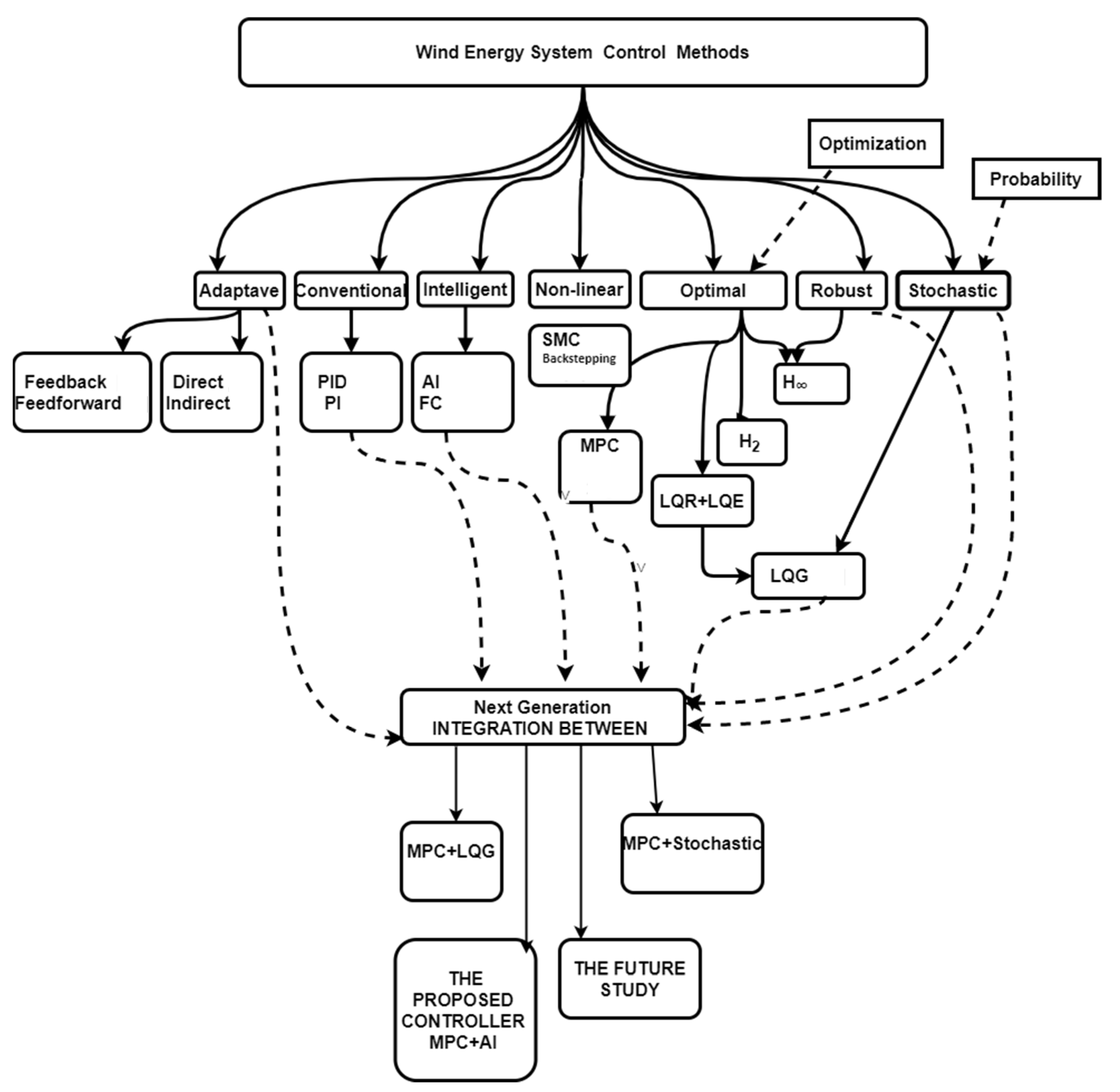
Most of the previous studies only concerned optimal control strategies or, only conventional controllers or an intelligent control (e.g., PID and MPC controllers). However, a few recent studies applied the advanced MPC controller.
(2)
Advanced MPC strategies are used for MPC combined with heuristic, meta-heuristic, or hierarchical algorithms. There is a good deal of possible integration between two or more approaches as shown in Figure 2. That might produce the next generation of controls to overcome the limitations of the previous control methods. Therefore, this study applies hybrid MPC with an artificial neural network to improve performance and smooth tracking.
(3)
Most of the techniques in previous works were often based on simplified models of the generator and the power electronics dynamics; their impact on the mechanical stresses of the mechanical part of the system was ignored. In this work, however, we consider a nonlinear model describing the dynamics of the wind turbine, the SCIG, and the SVC, the latter is used to regulate the generator terminal voltage.
(4)
The advanced MPC strategies have not been applied to all types of wind energy generation units.
(5)
The classical DMPC needs a high computational effort or can be difficult to implement, especially at high sampling frequency control; this can be solved by using Laguerre networks.

1.3. Contribution and Paper Organization

(1)
This paper investigates a new hybrid control via predictive control Laguerre-based MPC and artificial neural network (LMPC-ANN) approaches. To the best of the authors’ knowledge, this scheme was not found in the WEC control systems literature.
(2)
Complexity of MPC conventional algorithms is reduced by using MPC Laguerre-based MPC which reduces the computational time and makes it easy to implement.
(3)
The integration between ANN and MPC, increases the ability of the proposed control system for smooth tracking, overshoot reduction, optimization, and modeling. In addition, the new control scheme has strongly robust properties. Additionally, it can be applied for uncertainties and disturbances which result from wind speed variation.
(4)
The obtained results via the proposed controller show that it stabilizes the system (the type 1 wind energy system connected to the grid, which suffers from instability problems) and manages to render the states of the system the same as the normal operating conditions, despite fluctuating wind speeds.
The paper is sectioned as follows. Section 1 gives an overview of the approaches and methodologies that are used in this study. Next, Section 2 explains and describes the proposed MPC-based ANN scheme. Section 3 contains the simulation results and corresponding discussion. Section 4 gives the conclusions and suggestions of this study. Finally, the Appendix A describes the modeling of the system under study. Appendix B describes system parameters. Appendix C describes MPC-LQG Controller. Appendix D describes ANN-LQG Controller. Appendix E describes ANN for the LMPC-ANN Controller.

2. Materials and Methods

This section introduces the proposed methodology for controlling the wind energy system type 1 introduced in Appendix A, which can deal with the operating condition variability of the system according to the values of the wind speed. First, the control objectives adopted in this work are presented. Then, we detail the proposed approach.

2.1. Control Objectives

The control objective of the wind energy system when the wind speed values are less than the rated value, is to maximize the power extracted from the wind. On the other hand, at wind speed values more than the rated value, it is required to stabilize the extracted power to the rated value via the blade’s pitch angle actuator. Moreover, the FC-TCR is used to regulate the voltage at the generator terminal. Next, we introduce the Neuro-Predictive scheme for controlling the WES system.

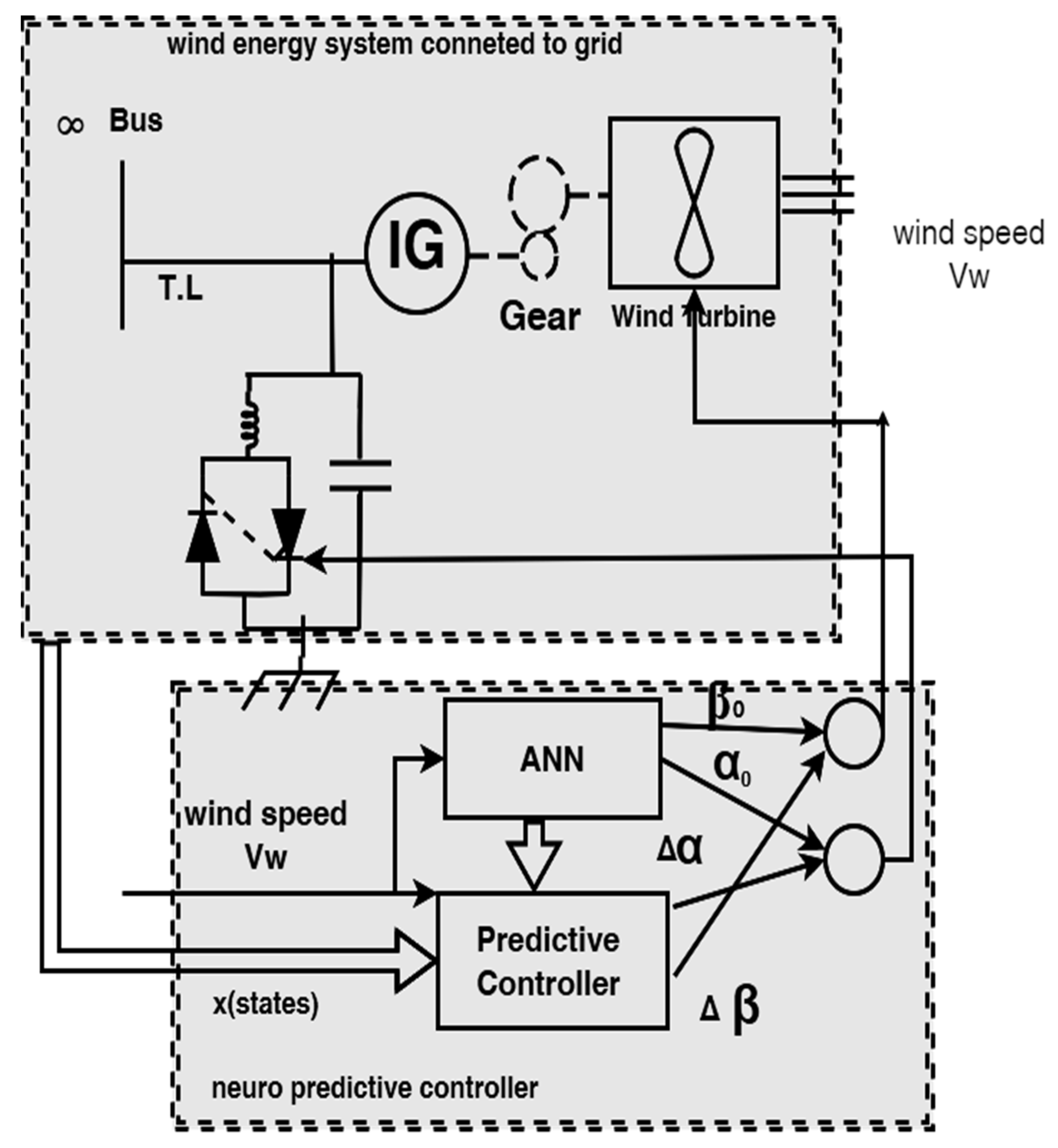
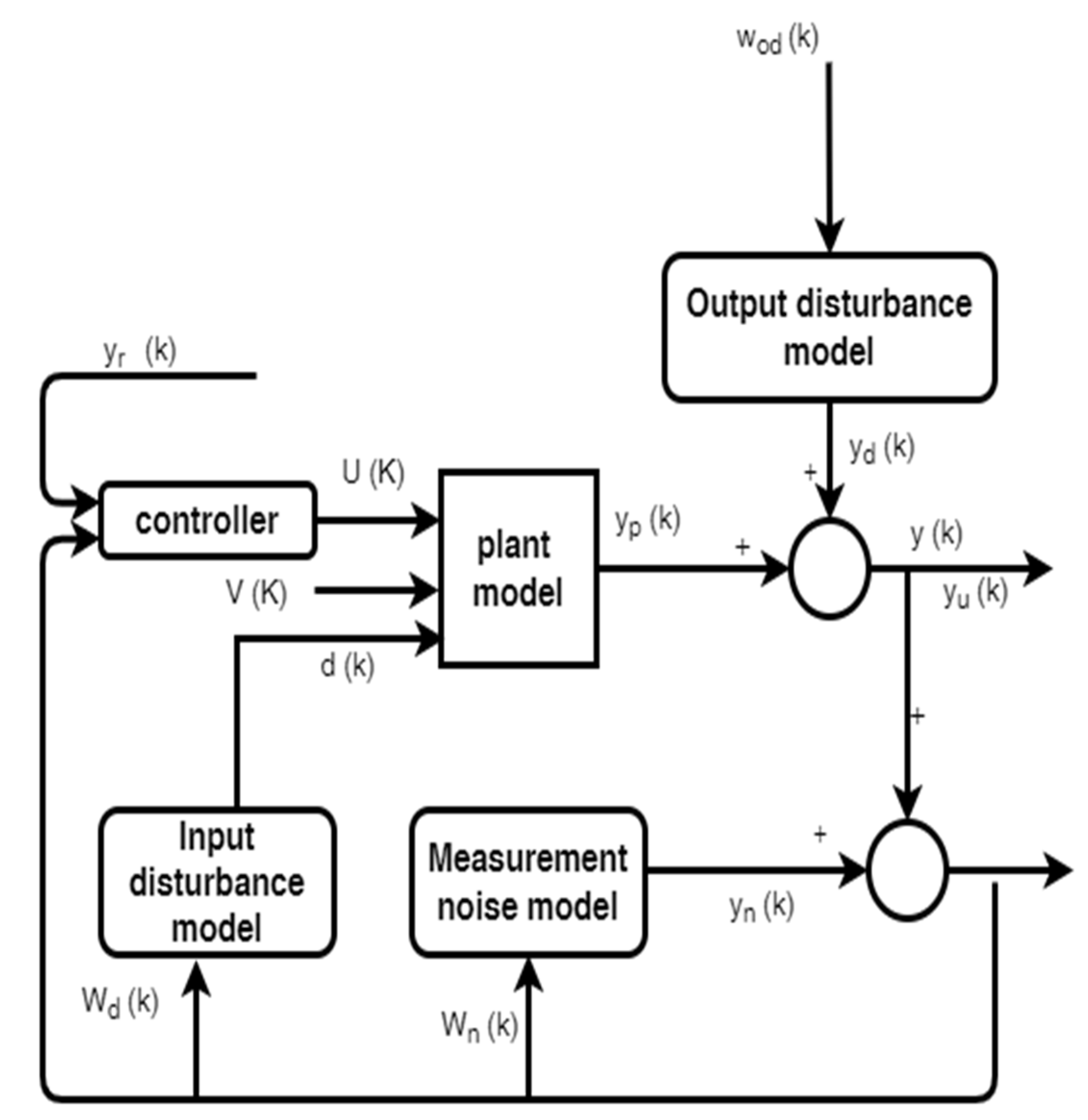
2.2. Modeling of the System

The mathematical model of the system considered here is shown in Figure 3. It consists of thirteen differential equations for all system components which are wind turbines, SCIG, grid, overhead transmission lines, and SVC (fixed-capacitor (FC) and Thyristors Controlled Reactor (TCR)). These are described in detail in Appendix A. This model can be represented by:
x ˙ n = f ( x n , u n ,   v )
where
  • v is the instantaneous average wind speed.
  • x n is the state vector of the systems.
  • u n is the vector of the control inputs.
Where
u n = [ β r α ] T
In order to control the system using MPC-based linear control approach linearized models should be obtained at each operating point corresponding to the value of the wind speed. We use the first order term of Taylor to approximate Equation (1) around a specified operating point to establish a linearized model, this is represented by
p x = A x + B u
where
  • A , B are the system matrices given in Appendix A.
  • x = [ Δ i s q   Δ i s d   Δ i r q   Δ i r q   Δ ω r   Δ V s q   Δ V s d   Δ i l q   Δ i l d   Δ i t q   Δ i t d   Δ ω t   Δ δ   Δ β ] T
  • u = [ Δ β r Δ α ] T .
First, Figure 3 describes the configuration of the proposed scheme. The ANN is used to estimate the value of the steady-state ( x n , u n ) at any operating point, that represents the differential equations of the system as., Δ f ( x n , u n ,   v ) = 0 . The value of ( x n , u n ) can be easily used to obtain the corresponding linearized model, which is used for the MPC algorithm to compute the optimal control input. We train the ANN offline to learn the steady-state values of the system given the wind speed. Using ANN in this scheme should save the time to solve f ( x n , u n ,   v ) = 0 , which otherwise should be performed online. At any value of the wind speed, the value of ( x n , u n ) drives the MPC to produce the optimal incremental values of the inputs to provide the control input to the plant of each instant as shown in Figure 3.

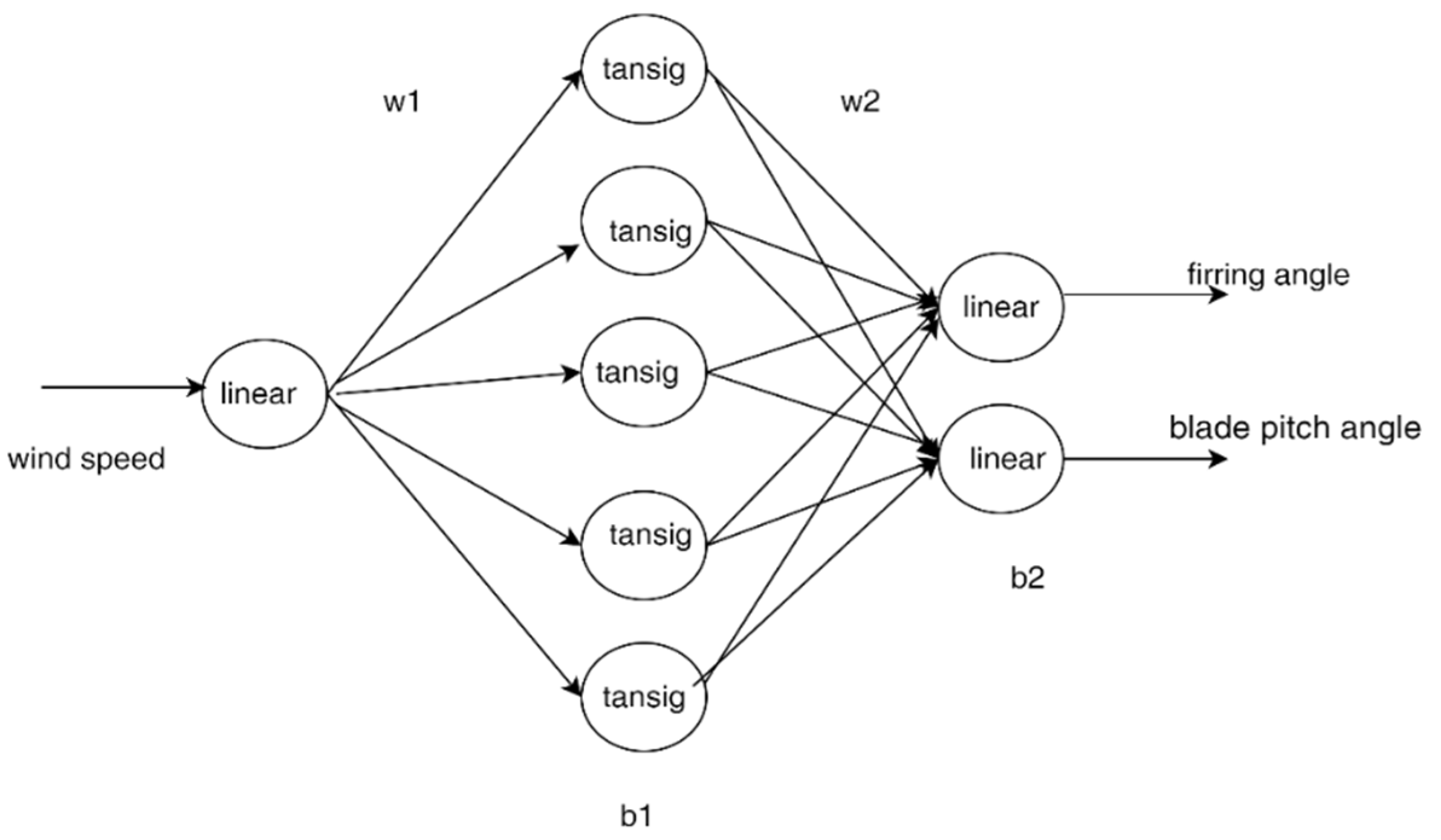
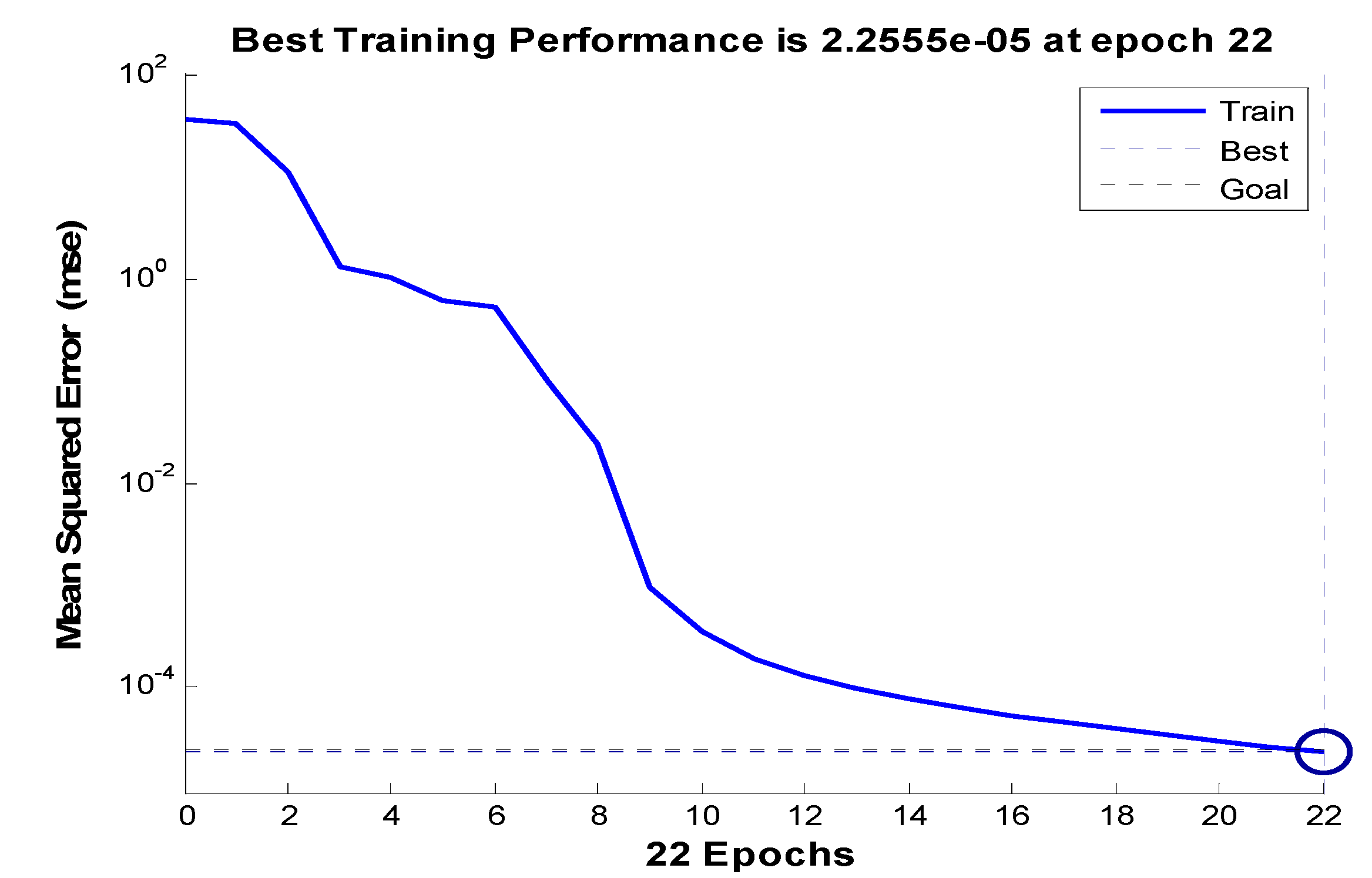
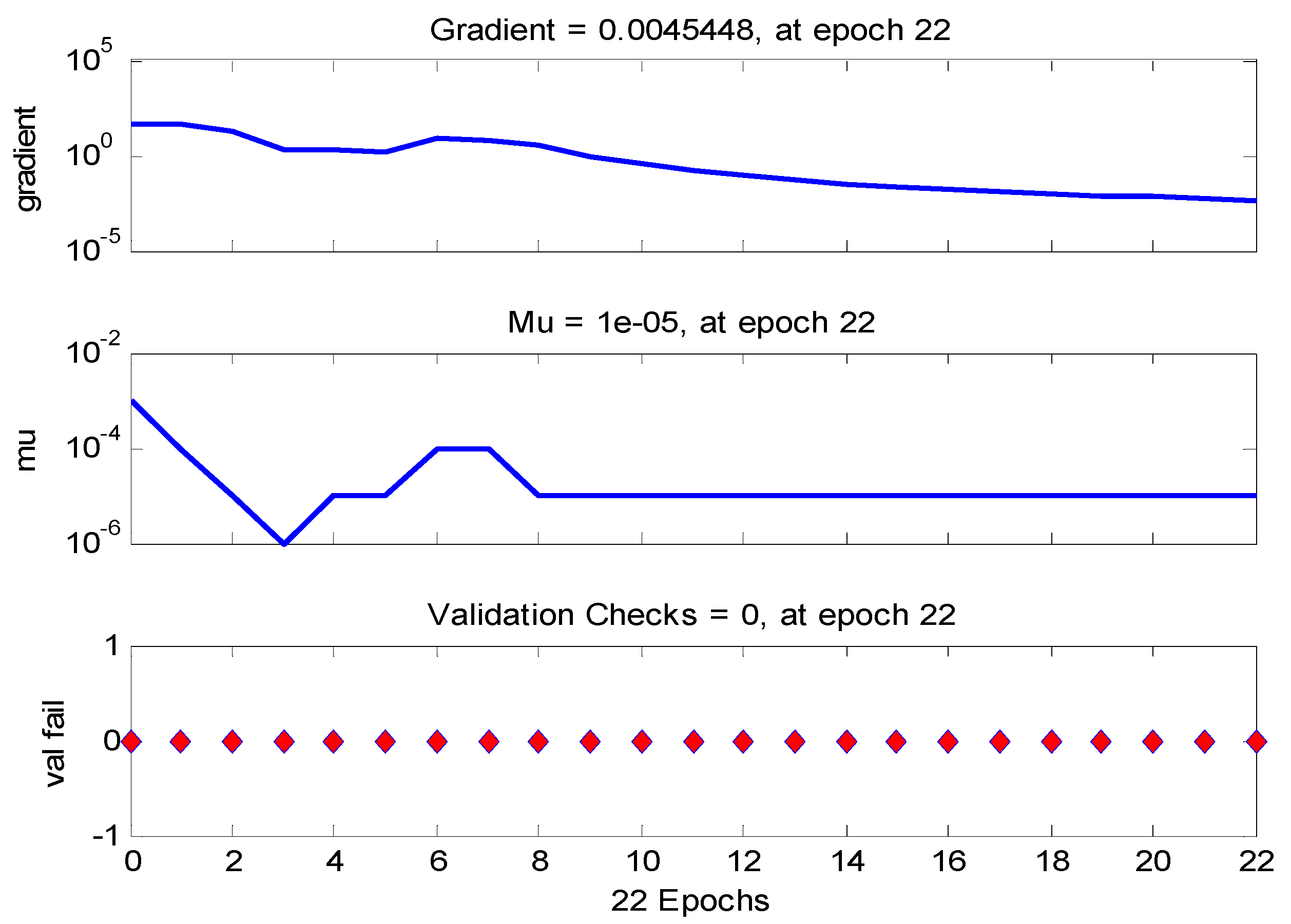
2.3. Training the ANN

Given a set of data ( x n , u n , v * ) for the wind speeds more than rated value, the ANN process as shown in Figure 4, can be trained off-line to learn the relation between v * and ( x n , u n ). It turns out that a single layer feedforward ANN with hyperbolic tan as an activation function was able to learn reasonably well such input-output relation. The Matlab neural network toolbox has been used to pre-process the data, train, and validate the ANN (Appendix E).

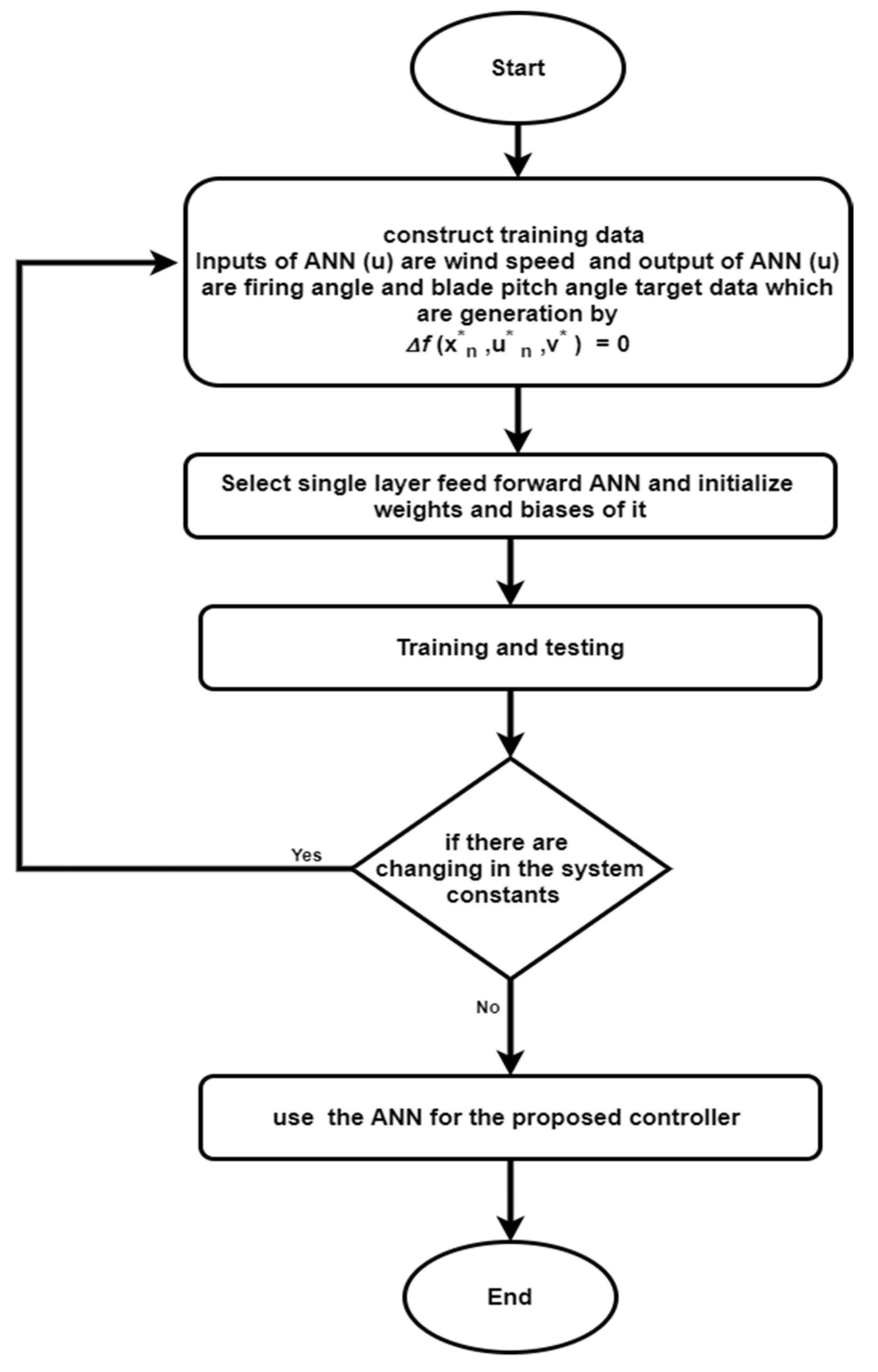
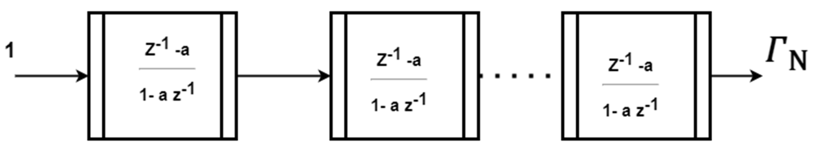
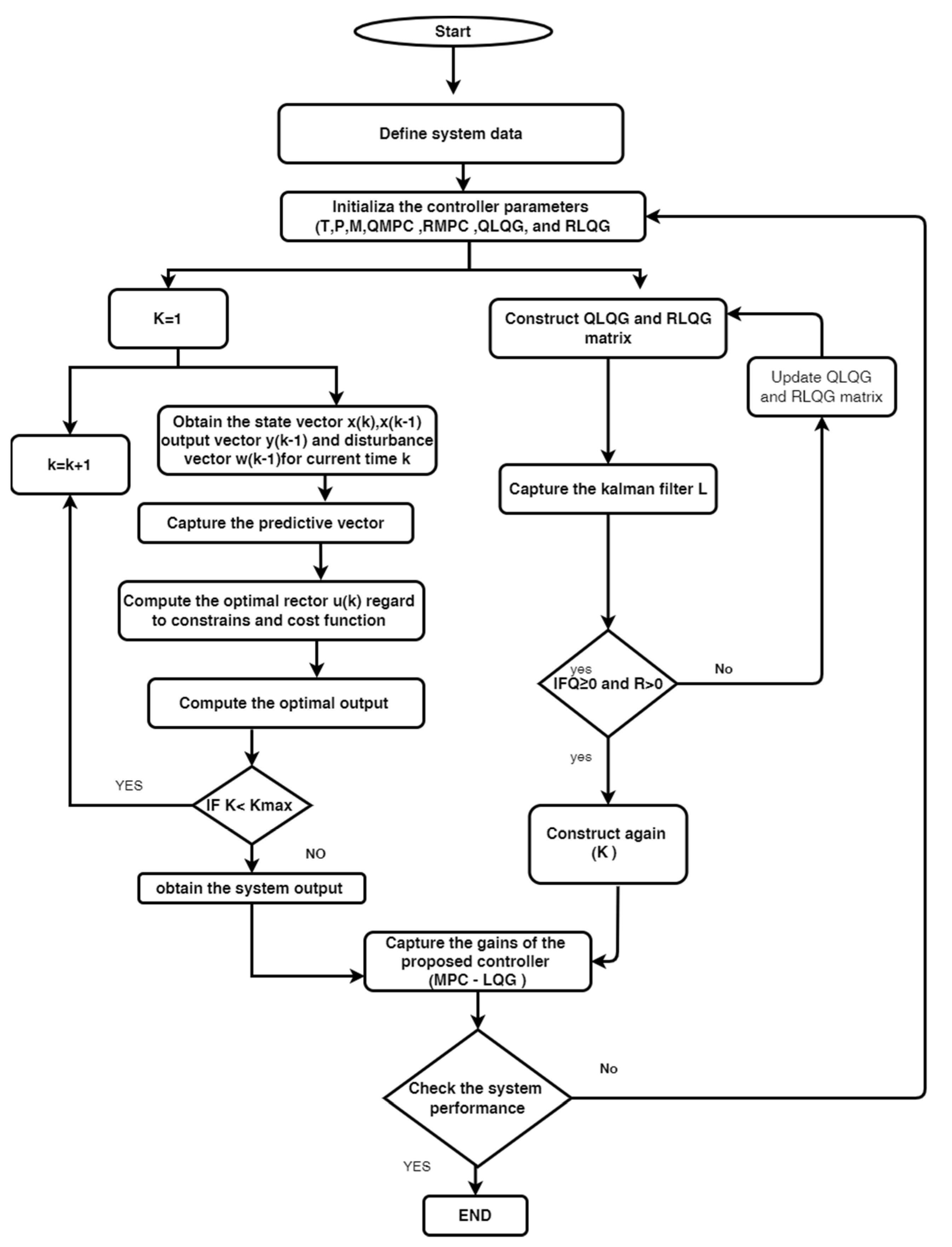
2.4. MPC-Based Laguerre Function
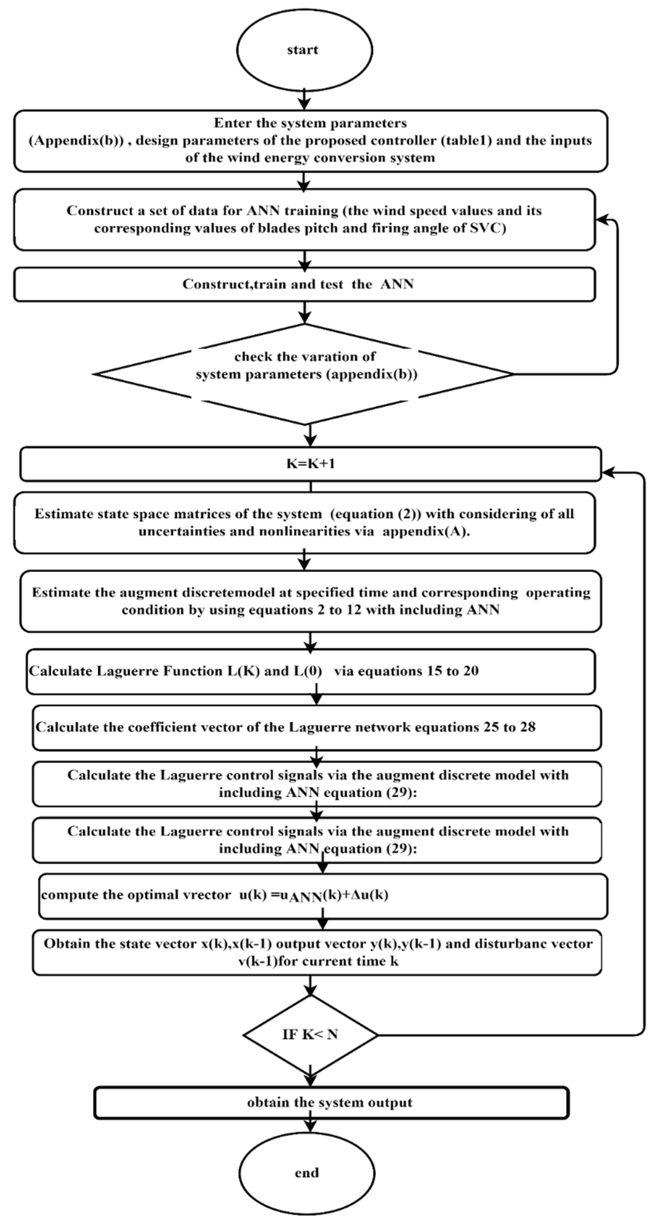
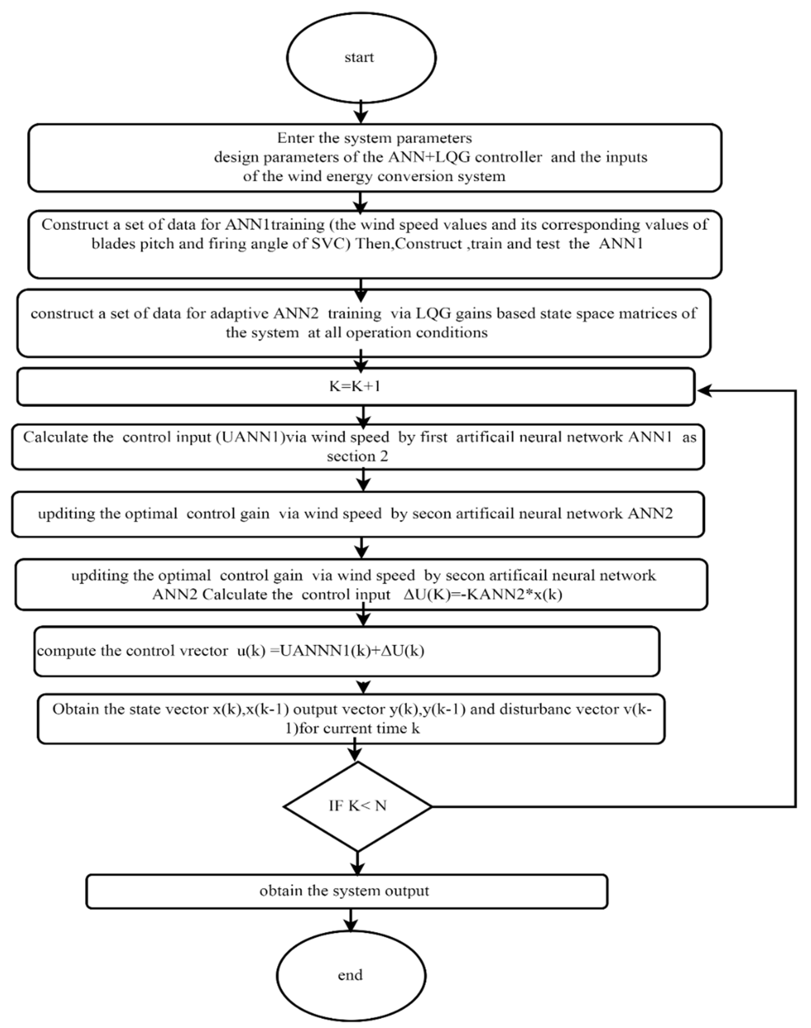
In this section, we continue to describe the new hybrid control via predictive control Laguerre-based MPC and artificial neural network (LMPC-ANN). For the construction of the proposed controller, the mathematical model of the wind energy generation unit should be put in the discrete state space form as follows [32].
x m ( k + 1 ) = A m × x m ( k ) + B m × u ( k )
y m ( k ) = C m × x m ( k )
where: x m ( k ) R n x ,   u ( k ) R n u and y ( k ) R n y Rny are the system state, input, and output, respectively, at a sampling instant k, Am, Bm, Cm are the state-space matrices.
In order to include embedded integral action for the control design, we augment the model as follows [33]
x ( k + 1 ) = A × x ( k ) + B × u ( k )
y ( k ) = C × x ( k )
where
x ( k + 1 ) = [ Δ x m ( k ) y ( k ) ] T
Δ x m ( k ) = x m ( k ) x m ( k 1 )
Δ u ( k ) = u ( k ) u ( k 1 )
A = [ A m 0 m T C m A m I ]
B = [ B m C m B m ]
A m = [ 0 m I ]
where I is the identity matrix. 0 m is the matrix with zero entries with appropriate dimensions.
The standard MPC problem is to minimize at each sampling instant the cost function
J = m = 1 N p x ( k i + m | k i ) T Q x ( k i + m | k i ) T + Δ U T U R Δ U
Over the parameter vector of the control sequence Δ U, where
Δ U = [ Δ u ( k i ) Δ u ( k i + 1 ) …… Δ u ( k i + N c 1 ) ] T
Np and Nc are, respectively, the prediction and control horizons, Np > Nc, x(ki + m|ki) is the predicted state variable vector at the sampling instant, given current state x(ki), Q = CC and R > 0 are weighting matrices, with Q has the dimension of x and R has a dimension of Δ u Q and R are used to tune the performance of the controller and they are varied based on two arbitrary constants (alpha, lambda) as described in [33].
A closed-form solution to this problem can be obtained, and the receding horizon principle is applied, i.e., the first sample of the sequence Δ U is implemented. Moreover, input-output constraints can be easily included, in this case, the optimal solutions are obtained using quadratic programming. Next, the MPC design procedure is generalized by introducing a set of discrete orthonormal basis functions into the design. Such generalization will help to reformulate the predictive control problem to simplify the solutions and tune the predictive control system.
Furthermore, a long control horizon can be realized without using a large number of parameters, which can lead to an appropriate MPC approach in the case of rapid sampling, complicated process dynamics and/or high demands on closed-loop performance, and cheap computational load for online implementation. Moreover, it predicts numerically conditioned solutions than those of the basic approach. The basic idea is to approximate the sequence Δ u ( k i ) Δ u ( k i + 1 ) Δ u ( k i + N c 1 ) by a set of discrete Laguerre functions, see [Wang Book] for justifying the use of such functions. The block diagram z-transform of discrete-time Laguerre network [34] is shown in Figure 5, which is based on the following relations:
Γ k ( z ) = Γ k 1 ( z ) z 1 a 1 a z 1
Γ 1 ( z ) = 1 a 2 1 a z 0
where a is the pole of the discrete-time Laguerre network, and a < 1 for the stability of the network. The parameter a is selected by the user, which is referred to as the scaling factor. The Laguerre networks are known for their orthonormality. For MPC design, the Laguerre functions [33,34] are used in the time domain. Based on the relation (29), the set of Laguerre functions can be described by the difference equation
L ( k + 1 ) = A l L ( k )
L ( k ) = [ l 1 ( k ) l 2 ( k ) …… l N ( k ) ] T
with li(k) is the inverse z-transform Γ i(z), and the matrix Al   RN × N is given by
A l = [ a 0 0 0 β 1 a 0 0 a β 1 β 1 a 0 a 2 β 1 : a β 1 : β 1 : : 0 : ( 1 ) N 2 a N 1 β 1 ( 1 ) N 3 a N 3 β 1 β 1 a ]
with β 1 = 1 − a2 and N is the number of terms used in the Laguerre network. So, this implies the initial condition
L ( 0 ) = β 1 [ 1 a a 2 a 3 ( 1 ) N 1 a N 1 ] T
The Laguerre networks are commonly used in system identification to capture the dynamic response of a system. Similarly, the control sequence in Δ U can be approximated by a set of Laguerre functions as follows
Δ u ( k i + k ) = j = 1 N c j ( k i ) l j ( k ) = L ( k ) T η
with ki being the initial time of the moving horizon window and k being the future sampling instant and η = [ c 1 c 2 c 3 c 4 …… c N ] T , with c1, c2, …… cN are the coefficients of the Laguerre series expansion. Therefore, given the state-space realization (2ab) with the initial state variable x(ki), the prediction of the future state variable, x(ki + m|ki) at a sampling instant m ki in terms of Laguerre functions can be represented by
x ( k i + m | k i ) = A m x ( k i ) + i = 0 m 1 A m i 1 B L ( i ) T η
where Δ u(ki + i) is replaced by L ( i ) T η . Similarly, the prediction for the plant output at future sample m, i.e., y (ki + m|ki) can be represented. This shows that both the predictions of the state variables and the output variables are expressed in terms of the coefficient vector η of the Laguerre network instead of Δ U. Thus, η will be optimized and computed in the MPC design. Now, the cost function can be rewritten in terms of η as
J = m = 1 N p x ( k i + m | k i ) T Q x ( k i + m | k i ) T + η T U R L η
In order to obtain η that minimizes the cost function, we solve the partial derivative
J η = 0
for η consequently, the optimal solution of η is given by [35]
η = Ω 1 Ψ x ( k i )
let
Ω = m = 1 N p φ ( m ) Q φ ( m ) T + R L
Ψ = m = 1 N p φ ( m ) Q A m
φ ( m ) T = i = 0 m 1 A m i 1 B L ( i ) T
Finally, by implementing the receding horizon principle, the control law a sampling instant ki, which should be implemented online is given by
Δ u ( k i ) = = L ( 0 ) T η
where L ( 0 ) T is computed from (13), which can be considered as at a time-varying state feedback policy where A, B, Q and R are calculated via the discreet matrices model [33]. This controller deals adaption of control signals via ANN. The ANN and the predictive control-based Laguerre function are used for optimal control of a wind energy system. Figure 6 presents a flowchart of integration between two strategies that were discussed in this section to produce the proposed controller performance. Additionally, it can be summarized in the following steps:
Step 1: 
Enter the system parameters (Appendix B), design parameters of the proposed controller (Table 1), and the inputs of the wind energy conversion system.
Step 2: 
Construct a set of data that contains the wind speed values and the corresponding values of blades pitch and firing angle of SVC for optimum power and voltage generation.
Step 3: 
Construct, train, and test an ANN via the set data in step 2.
Step 4: 
If there is no change in the system parameters go to step 5, or repeat step 2 and step 3.
Step 5: 
Estimate the mathematical model of the system (Equation (2)) with consideration for all uncertainties and nonlinearities. It is estimated via thirteen differential equations for all system components which are given in Appendix A.
Step 6: 
Estimate the augment discrete model at specified times and corresponding operating conditions by using step 5 and equations 2 to 12 including ANN.
Step 7: 
Calculate the Laguerre function L(K) and L(0) via equations 15 to 20.
Step 8: 
Calculate the coefficient vector η of the Laguerre network equations 25 to 28.
Step 9: 
Calculate the Laguerre control signals via the augment discrete model with including ANN as: Δ u ( k i ) = = L ( 0 ) T η
Step 10: 
Calculate the control signals of ANN u A N N ( k i ) = f ( v )
Step 11: 
Calculate the optimum control signals u o p ( k i ) = u A N N ( k i ) + Δ u ( k i )
Step 12: 
Repeat steps 5 to 10 for the next instant until it reaches the N sample.
Step 13: 
End.
Table 1. Shows the initial values for designing the of the neuro-predictive controller.
Parameter for DesigningThe Values
lambda=0.9
alpha1.5
Β1
Time sampling0.01
the number of terms for each input (N)10
prediction horizon (Np)5
contains the Laguerre pole locations for each input (a)0.9

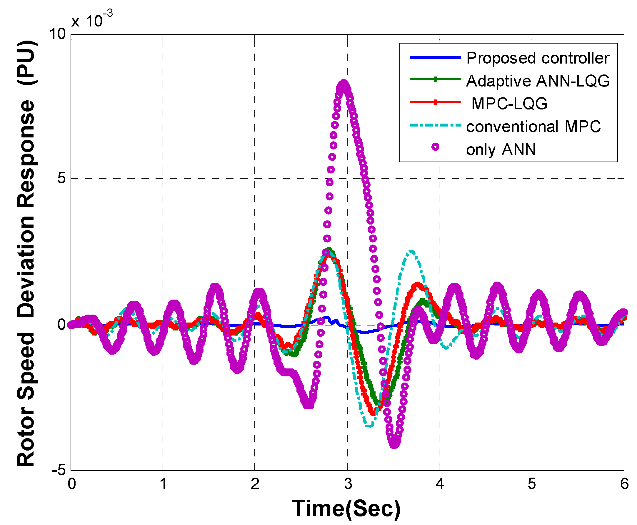
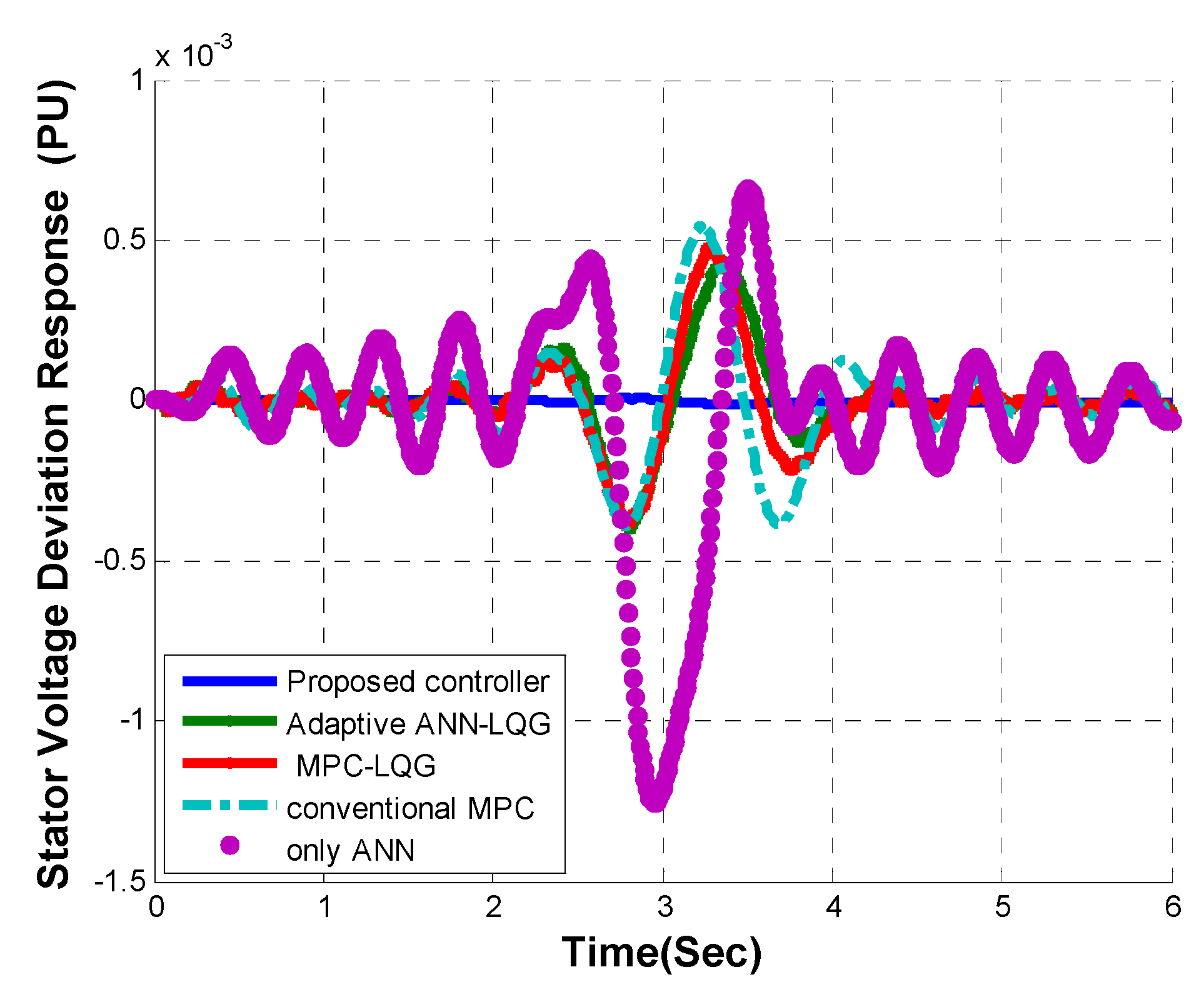
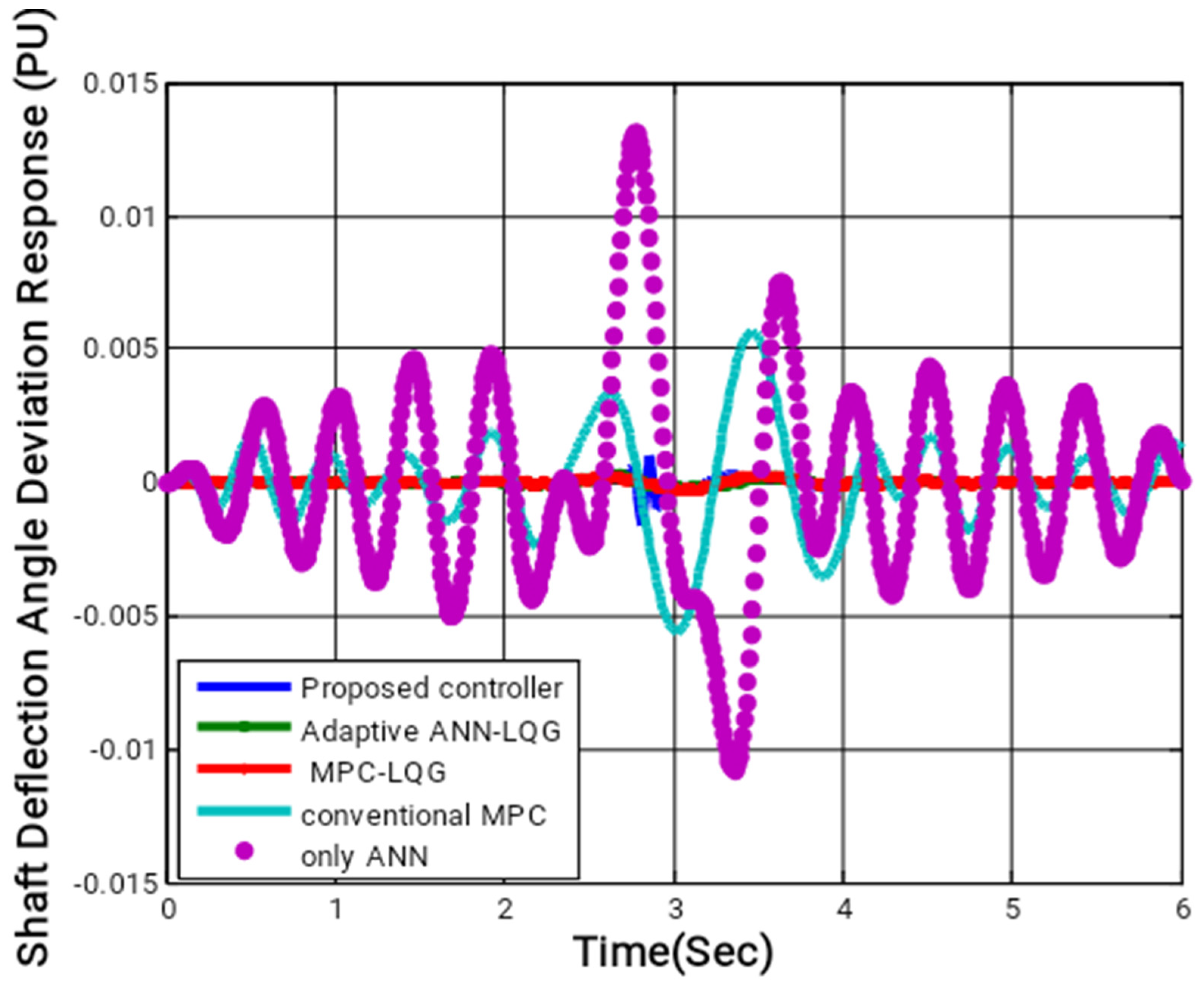
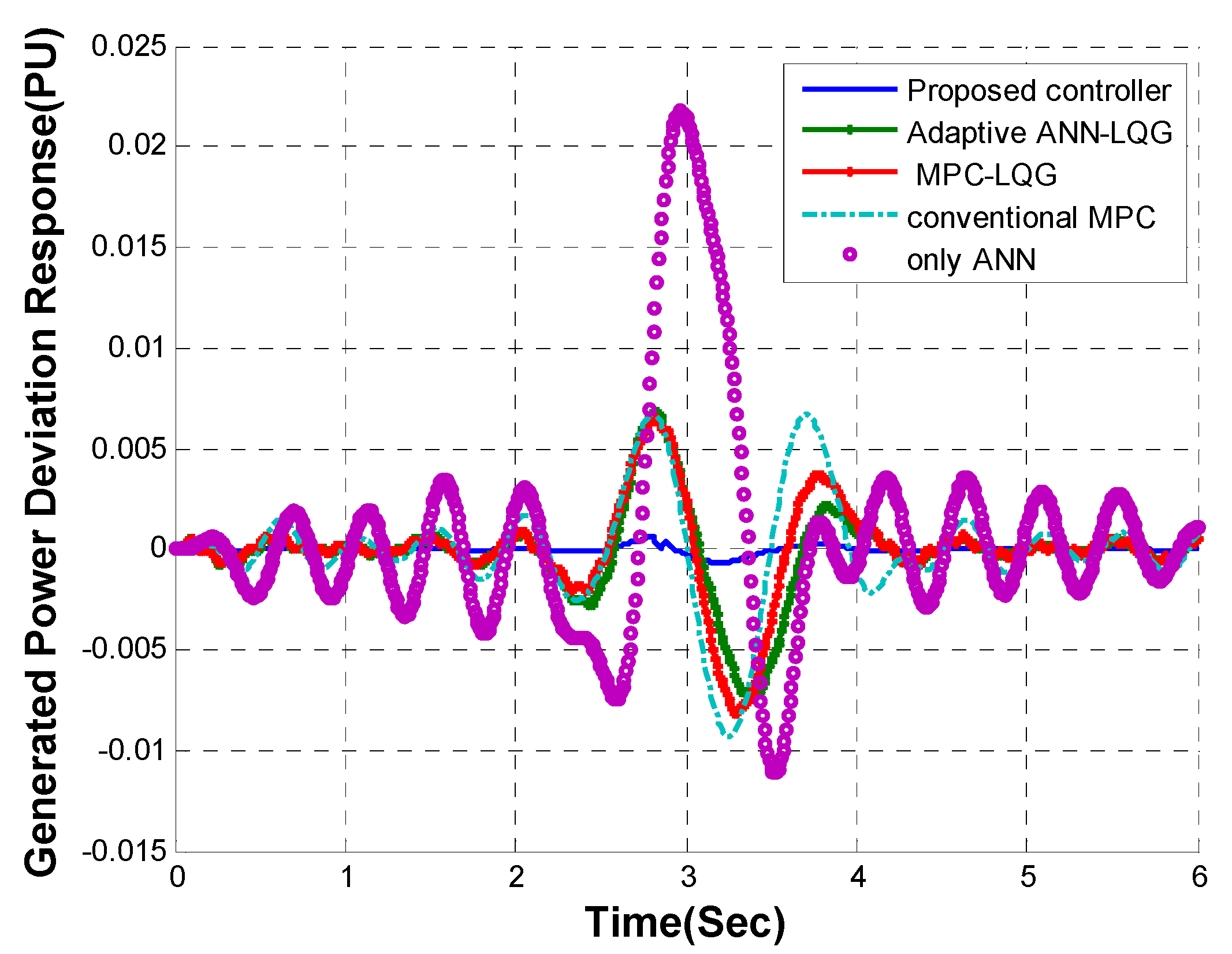
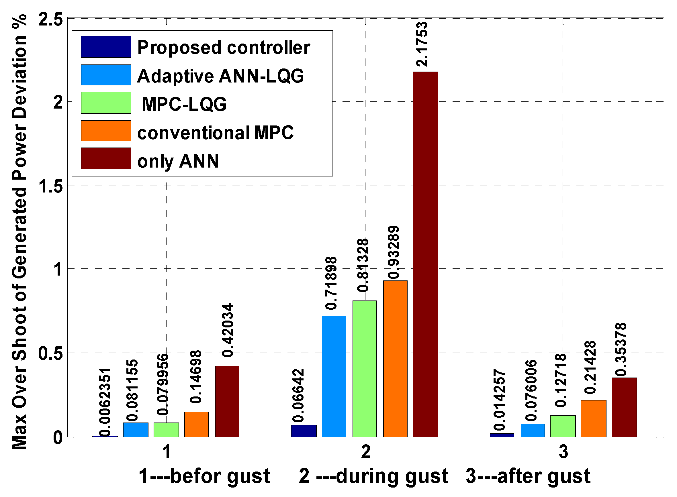
3. Results and Discussion

In this section, the neuro-predictive (LMPC-ANN) controller is applied to a 3 MW wind energy generation unit connected to a power system through SVC, as shown in Figure 3. All constants of the system elements are given in Appendix B. Table 1 shows the initial values for the design of the neuro-predictive controller. There are three time zones used to study the effectiveness of the controller as follow:
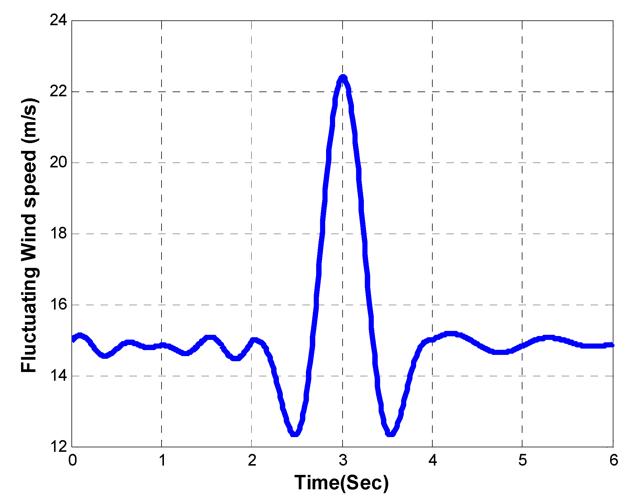
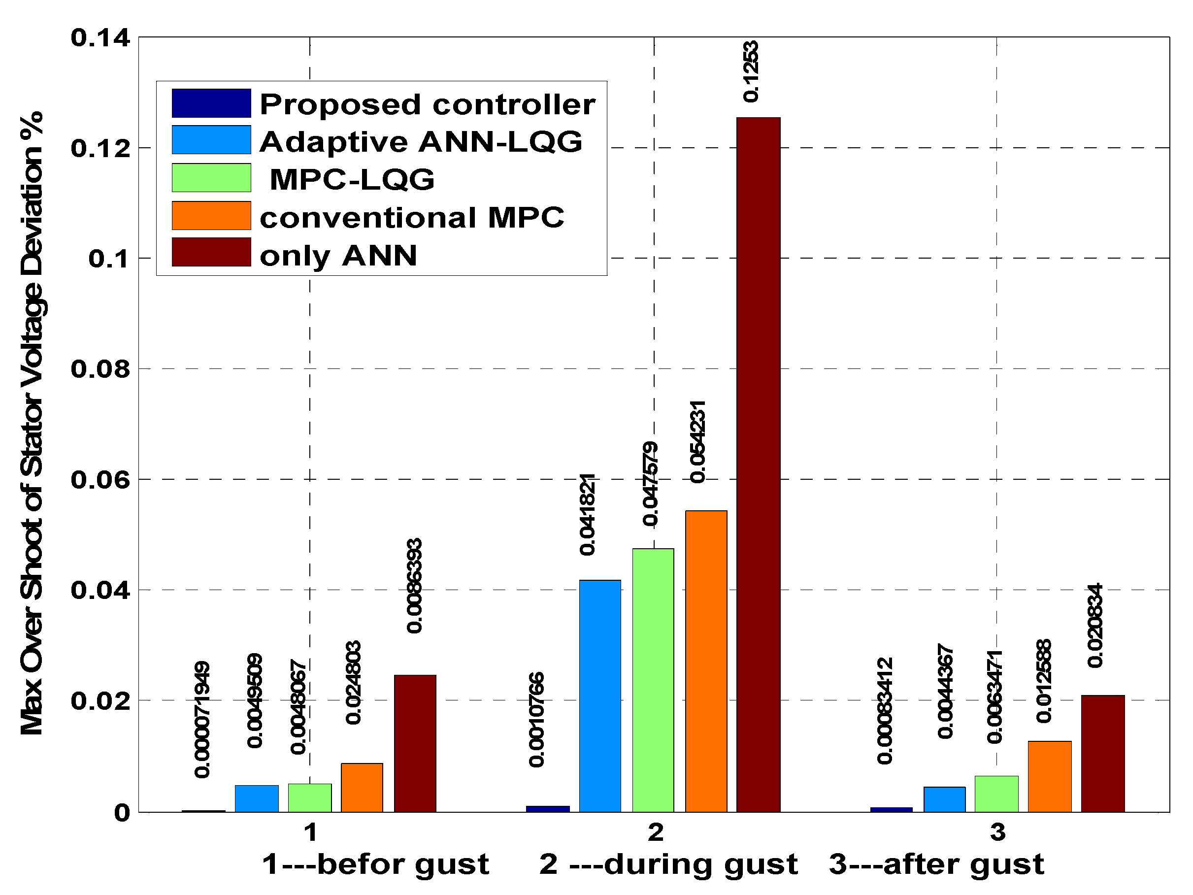
REGION A (before gust):
in this region, wind speed values are within a normal variation zone as shown in Figure 7; measurements are taken within the first two seconds.
REGION B (during gust):
this region is measured during wind gusts which are sudden variations in the wind speed as shown in Figure 7. Values are between t = 2 to t = 4 in this system.
REGION C (after gust):
this region is measured after wind gusts, the value of wind speed returns to the normal variation as is shown in Figure 7; they are measured as between t = 4 s and t = 6 s.
The performance of the studied system is estimated based on different strategies, which are:
  • The ANN only
  • Conventional MPC [20] strategy is given in Appendix C
  • Adaptive ANN-LQG [36] strategy is given in Appendix C
  • Conventional MPC-LQG [31] strategy is given in Appendix D
  • The proposed controller is neuro-predictive (LMPC-ANN)
  • Figure 8, Figure 9, Figure 10 and Figure 11 show the response of the system with different controllers in terms of the deviations of the rotor speed (Δωr), shaft deflection angle (Δδ), stator voltage (ΔVs), and generated power (ΔPg)
In the previous figures, the system performance before a gust with different controllers is shown. We can notice that the system with only ANN suffers from instability problems, and it cannot dampen the oscillation result from the normal fluctuation of wind speed. On the other hand, the systems with MPC, ANN-LQG, and MPC-LQG have a better dynamic response than in the previous case. The systems with LMPC-ANN achieve the best dynamic response in comparison to the other modern controllers such as ANN-LQG and MPC-LQG. Additionally, the same figures show that the systems with only ANN during the gust have high oscillation with the largest value of max overshoot due to gust fluctuation of wind speed, on other hand the systems with conventional MPC, ANN-LQG, and MPC-LQG have a slightly better dynamic response than in the previous case. Regardless, the system with LMPC-ANN still demonstrates the best dynamic response in comparison to the other modern controllers (ANN-LQG and MPC-LQG). Furthermore, the system behavior after gusts return is approximately the same as before with different controllers. To summarize the analysis of these results, Figure 12 and Figure 13 show the maximum values of overshoot in generating power and voltage in different cases, the wind fluctuation effects are mitigated while maintaining the power generated and generator terminal voltage at optimum values.
Table 2 and Table 3 highlight the effectiveness of the proposed neuro-predictive control compared to the other strategies in reducing the maximum overshoot of generating power and voltage. It is clear from Table 2 and Table 3 that the reduction in maximum overshoot of generating power and voltage with proposed neuro-predictive control is better compared to the best results obtained through the other modern control strategies.
Generally, it is clear that the responses of the system without a controller oscillate highly. On the other hand, the system with the NEURO-MPC controller can stabilize the system and dampen the oscillations. However, the responses with the proposed controller outperform those with the modern controllers, especially ANN-LQG and MPC-LQG. The oscillations with the proposed gust died out within less than 0.9 sec. The obtained results show that the proposed control stabilizes the system and renders the system states at the normal operating conditions at all levels of fluctuating wind speeds.

4. Conclusions

In this work, a predictive control scheme based on an artificial neural network has been proposed to control a wind-driven squirrel cage induction generator (SCIG) system connected to a grid. The ANN is used to obtain the steady-state values of the system, corresponding to any values of the wind speed to complete the associated linearized model of the system. The control objective is to mitigate wind fluctuation effects by regulating the rated power generated by the system while maintaining its terminal voltage at the rated value. For this purpose, a predictive control scheme is designed based on orthonormal Laguerre functions. The predictive control is integrated with the ANN. The use of the ANN can simplify the online computation of the operating points. The proposed predictive control shows a better response in comparison with a conventional controller, which can improve the power system stability, and reliability and increase the operational lifetime.
The proposed controller can adapt its operation according to the wind speeds and hence can achieve optimal performance at any value of the wind speed. The system with such predictive control has been tested under fluctuating wind speeds. From the present analysis, the obtained results show that the system without controllers suffers from instability problems, on other hand, the proposed control stabilizes the system and manages to render the system states at the normal operating conditions at different values of the wind speeds. The future expansion of this work, would be to investigate the neuro-predictive scheme’s impact on different types of wind energy systems. Additionally, to observe it applied to different types of renewable energy systems.

Author Contributions

Conceptualization, M.A.-E.-H.M., H.S.A. and S.K.; Data curation, M.A.-E.-H.M., H.S.A. and S.K.; Formal analysis, M.A.-E.-H.M., H.S.A. and S.K.; Funding acquisition, M.A.-E.-H.M., H.S.A. and S.K.; Investigation, M.A.-E.-H.M., H.S.A. and S.K.; Methodology, M.A.-E.-H.M., H.S.A., M.S. and S.K.; Project administration, M.A.-E.-H.M., H.S.A. and S.K.; Resources, M.A.-E.-H.M. and M.S.; Software, M.A.-E.-H.M. and M.S.; Supervision, M.A.-E.-H.M.; Validation, M.A.-E.-H.M. and M.S.; Visualization, M.A.-E.-H.M.; Writing—original draft, M.A.-E.-H.M. and M.S.; Writing—review & editing, M.A.-E.-H.M. and M.S. All authors have read and agreed to the published version of the manuscript.

Funding

This research received no external funding.

Conflicts of Interest

The authors declare no conflict of interest.

Nomenclatures

SYMPOLDESCRIBTION
(MPC)Model predictive control
(ANN)Artificial neural network
(SVC)Static VAR compensator
(SCIG)Squirrel cage induction generator
(FC-TCR) Fixed-capacitor Thyristors controlled reactor
(WECS)Wind energy conversion system
v is the instantaneous average wind speed
x n is the state vector of the systems
u n is the vector of the control inputs such
β Blades pitch angle
α Firing angle
A , B are the system matrices
i s d The d component of stator current
i s q The q component of stator current
i r q The q component of rotor current
ω r Wind turbine angular speed
i l d The d component of TCR current
i l q The q component of TCR current
i t d The d component of T.L current
i t q The q component of T.L current
X m Magnetizing reactance
Am, Bm, Cmare the state-space matrices
I   and   0 m represent, respectively, the identity matrix and a matrix with zero entries with appropriate dimensions.
ΔU The control sequence
NcControl horizon
NpPrediction horizon
x(ki + m|ki)Predicted state variable vector at sample time m, given current state x(ki)
ηParameter vector in the Laguerre expansion
c1, c2, · · ·,cNare the coefficients of the Laguerre series expansion.
ΔDeflection angle of the drive shaft,
Ψ. Ω MPC cost function matrices
V s The stator voltage terminal
Pggenerated power
Q and R are used to tune the performance of the controller
(FC)Fixed-capacitor
(TCR) Thyristors controlled reactor
T g Induction generator torque
Neuro-LQRThe conventional controller
yOutput signal
D s Damping Ds constant
G r Gear box ratio
KsThe spring constant
p Pairs no of pole
ω g Induction generator angular speed
J g Entire constant generator
ω t Wind turbine angular speed
T t Wind turbine torque
λ Tip speed ratio
V w Wind speed
ω s Stator speed
S Slip of the machine
X e Equivalent reactance of the transmission line
V s d The d component of stator voltage
R e Equivalent resistance of the transmission line
V s q The q components of stator voltage
X c Equivalent reactance of the FC
X l Equivalent reactance of the TCR
R r Rotor resistance
p Differentiation operator
LDiscrete and continuous-time Laguerre functions in vector form

Appendix A. Modeling of a Wind Energy System Type 1

The schematic diagram of the system considered here is shown in Figure 2. It consists of a horizontal axis type of wind turbine and a SCIG connected to the grid via an overhead transmission line through SVC (fixed-capacitor (FC) and Thyristors controlled reactor (TCR)) [32]. Next, the dynamics of each component of this system are described.

Appendix A.1. Wind Turbine

The wind turbine model describes the aerodynamics, mechanics, and pitch actuator dynamics of the system as shown in Figure 4.
Equations (A1) and (A2) describe the dynamics of the generator and rotor sides, respectively [37]:
p ω g = 1 J g ( T s g T g )
p ω t = 1 J t ( T t T s t )
where p is differentiation operator, ωg and ωt are the angular speeds on the generator and rotor sides, respectively, Jg, Jt are the inertias, Tg, Tt are the generator and turbine torques and Tsg, Tst are the transmitted torques via the gear ratio (Gr) as
T s g = T s t G r
The torque Tst is given by
T s t = D s p δ + K s δ
where Ds and Ks are constants terms and δ represents the deflection of the drive shaft.
Wind turbines can be characterized by using non-dimensional curves.
The developed torque is given as:
T t = 0.5 ρ A R C p V w 2 λ
where A is the swept area, ρ is the air density, Cp is power coefficient, λ is tip speed ratio which is given by
λ = ω t R V w
R is the rotor radius of the turbine
C p = ( 0.44 0.0167 β ) sin ( π ( λ 3 ) 15 0.3 β ) 0.00184 β ( λ 3 ) ω g = ω r P ω r = ( 1 S ) ω s j j
The pitch angle actuator represented by [38]
p β = 1 T b β + 1 T b β r
where βr is the control input of the wind turbine and Tb is a constant.
Finally, Equation (8) describes dynamics of twist of rotor shaft:
p δ = ω t ω g G r

Appendix A.2. The SCIG

The SCIG dynamic model in the d- and q-axis synchronous reference frame is given as follows [39]:
p i s q = A 1 R s i s q ( ω b A 2 ω r L m ) i s d + A 2 R r i r q ω r L m A 1 i r d + A 1 V s q
p i s d = ( ω b + ω r A 2 L m ) i s q A 1 R s i s d + ω r A 1 L m i r q + R r A 2 i r d + A 1 V s d
p i r q = A 2 R s i s q + ω r L s A 2 i s d + ( ω b + ω r L s A 1 ) i r d A 3 i r q A 2 V s q
p i r d = ω r L s A 2 + A 2 R s i s d ( ω b ω r L s A 1 ) i r q A 3 i r d A 2 V s d
where
A 1 = L r / L m 2 L s L r
A 2 = L m / L m 2 L s L r
A 3 = R r ( 1 + A 2 L m ) / L r
where: the electromagnetic torque of the generator can be expressed as:
T g = 3 P L m 2 ( i s q i r d i s d i r q )

Appendix A.3. SVC Model

FC-TCR -SVC [40] is used to regulate the generator terminal voltage by adjusting the Thyristor gating angle of the TCR branch. Consequently, its equivalent reactance provides the desired terminal voltage. The relation between the current and voltage of FC-TCR in the d- and q-axis synchronous reference frame can be given by
p i l q = ω b X l V s q ω b i l d
p i l d = ω b X l V s d + ω b i l q
p V s q = ω b X c i c q ω b V s d
p V s d = ω b X c i c d + ω b V s q

Appendix A.4. Transmission Line Model

Finally, the dynamics of the transmission line can be described by [39]:
p i t q = ω b X e ( V s q V b q ) R e ω b X e i t q ω b i t d
p i t d = ω b X e ( V s d V b d ) R e ω b X e i t d + ω b i t q

Appendix B. System Parameters Data

A. Induction Generator Parameters
4 poles, 6.6 Kv, 60 Hz.
Xm = 4.161 pu.;
X1s = 0.135 pu.;
X1r = 0.075 pu.;
Rs = 0.0059 pu.;
Rr = 0.0339 pu.;
Hg = 1.975 s:
B. Static VAR Compensator Parameters
Xlmax = 4:0 pu.; Xc = 3:8 pu.
C. Transmission Line Parameters
Xe = 0.15 pu.;
Re = 0.015 pu.;
V = 1.04 pu.
D. Wind Turbine Parameters
Horizontal axis wind turbine (6 MW)
Ht = 16:72 s;
R = 200 ft;
Gr = 103:6

Appendix C. MPC-LQG Controller

In this method, the MPC-LQG controller combines MPC and LQG controllers. In addition, the controller depends on the control horizon (M), prediction horizon (P), and sampling time (ts). The conventional MPC controller is illustrated in the Figure A1.
Figure A1. Conventional MPC configuration.
Energies 15 05839 g0a1
The controller blends the merits of the MPC and LQG approach. The design process of the proposed MPC-LQG controller has been conducted in MATLAB software using the MPC toolbox and the LQR function.
Where
x p   ( k + 1 ) = A p x p ( k ) + B P U u ( k ) + B p v v ( k ) + B p d d ( k )
y p ( k ) = C p x p ( k ) + D p u v ( k ) + D p v u ( k ) + D p d d ( k )
C p = s 0 1 . C
The goal of reducing the quadratic cost function was accomplished by achieving the optimal solution as follows
J = t o t f ( x , Q x + u R u + 2 X N u ) d t
Here, QLQG and RLQG are the weight and the control matrices, respectively. Then, to reduce the value of J, it is necessary to select the optimum value of the K control input.
u ( t ) = k ( t ) x ( t )  
The LQG together with the predictive control-based Laguerre function are used for optimal control of a wind energy system. Figure A2 presents a flowchart of the integration between two strategies which were discussed [31] to produce the proposed controller performance.
Figure A2. Flow chart of LQG-MPC cotroller [31].
Energies 15 05839 g0a2

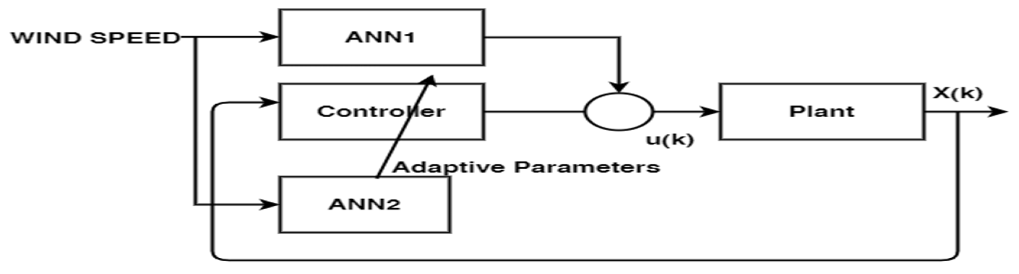
Appendix D. Adaptive ANN-LQG

The Neuro-Adaptive Control outline [40], strategies is designed based on the LQG controller. There are two ANNs to adapt the control signal online with wind speed variations as shown in Figure A3,. One of them is ANN1, which is trained as presented in Section 2. The other one is ANN2, which is trained via LQG gain computation at any possible value of wind speeds. Figure A4 shows the flow chart of the ANN-LQG controller.
Figure A3. Block diagram of ANN-LQG controller.
Energies 15 05839 g0a3
Figure A4. Flowchart of ANN-LQG controller.
Energies 15 05839 g0a4

Appendix E. Artificial Neural Network for the LMPC-ANN Controller

The following Figure A5 and Table A1 can be described the construction and properties of the ANN which is used for the proposed controller
Figure A5. Structure of the ANN for the LMPC-ANN controller.
Energies 15 05839 g0a5
Table A1. Structure of the ANN.
ConstructionDiscerption
w1hidden and input neurons weight
b1hidden nodes biases
hidden layer outputoh = tansig (w1*in, b11)
w2Hidden and output weights
b2output nodes biases
The output of ANNo1 = purelin (w2*oh, b2)

Parameters Computation for for The LMPC-ANN Controller

The training data was fed to Matlab Toolbox to calculate the weights and biases of artificial neural network.
The statistical data for artificial neural network training:
No of iterations = 1000
Max. Squared error = 1 × 10⁻⁷
Learning rate = 0.001
Figure A6. Neural network training performance.
Energies 15 05839 g0a6
Figure A7. Neural network training states.
Energies 15 05839 g0a7
The resulting weight matrices and biases of this ANN are given by:
b 1 = [   10.5628   0.6878   4.0000   1.5718 ]
w 1 = [   0.625   0.33130   0.163   2.445   12.20 ] t
b 2 = [ 2.129 4.5646 ]
w 2 = [ 0.0001 0.0064   0.00001   0.6337     1.6386 0.0320   1.3092   11.1940   1.1208       4.9879 ] t

References

  1. Ahmed, S.D.; Al-Ismail, F.S.M.; Shafiullah; Al-Sulaiman, F.A.; El-Amin, I.M. Grid Integration Challenges of Wind Energy: A Review. IEEE Access 2020, 8, 10857–10878. [Google Scholar] [CrossRef]
  2. Jha, D. A comprehensive review on wind energy systems for electric power generation: Current situation and improved technologies to realize future development. Int. J. Renew. Energy Res. 2017, 7, 1786–1805. [Google Scholar]
  3. García-Sánchez, T.; Muñoz-Benavente, I.; Gómez-Lázaro, E.; Fernández-Guillamón, A. Modelling Types 1 and 2 Wind Turbines Based on IEC 61400-27-1: Transient Response under Voltage Dips. Energies 2020, 13, 4078. [Google Scholar] [CrossRef]
  4. International Electrotechnical Commissio. Wind Turbines—Part 21: Measurement and Assessment of Power Quality Characteristics of Grid Connected Wind Turbines; IEC 61400-21; International Electro Technical Commission (IEC): Geneva, Switzerland, 2008. [Google Scholar]
  5. Tsili, M.; Papathanassiou, S. A review of grid code technical requirements for wind farms. IET Renew. Power Gener. 2009, 3, 308. [Google Scholar] [CrossRef]
  6. Mayosky, M.; Cancelo, I. Direct adaptive control of wind energy conversion systems using Gaussian networks. IEEE Trans. Neural Netw. 1999, 10, 898–906. [Google Scholar] [CrossRef]
  7. Dekali, Z.; Baghli, L.; Boumediene, A. Indirect power control for a Grid Connected Double Fed Induction Generator Based Wind Turbine Emulator. In Proceedings of the 2019 International Conference on Advanced Electrical Engineering (ICAEE), Dhaka, Bangladesh, 26–28 September 2019; pp. 1–6. [Google Scholar]
  8. Abokhalil, A. Grid Connection Control of DFIG for Variable Speed Wind Turbines under Turbulent Conditions. Int. J. Renew. Energy Res. 2019, 9, 1260–1271. [Google Scholar] [CrossRef]
  9. Chen, J.; Yao, W.; Zhang, C.-K.; Ren, Y.; Jiang, L. Design of robust MPPT controller for grid-connected PMSG-Based wind turbine via perturbation observation based nonlinear adaptive control. Renew. Energy 2018, 134, 478–495. [Google Scholar] [CrossRef]
  10. Sharaf, A.M.; Wang, G. Wind energy system voltage and energy enhancement using low cost dynamic capacitor compensation scheme. In Proceedings of the International Conference on Electrical, Electronic and Computer Engineering, ICEEC’04, Cairo, Egypt, 5–7 September 2004. [Google Scholar]
  11. Tamaarat, A.; Benakcha, A. Performance of PI controller for control of active and reactive power in DFIG operating in a grid-connected variable speed wind energy conversion system. Front. Energy 2014, 8, 371–378. [Google Scholar] [CrossRef]
  12. Zidani, Y.; Zouggar, S.; Elbacha, A. Steady-State Analysis and Voltage Control of the Self-Excited Induction Generator Using Artificial Neural Network and an Active Filter. Iran. J. Sci. Technol. Trans. Electr. Eng. 2017, 42, 41–48. [Google Scholar] [CrossRef]
  13. Colak, M.; Cetinbas, I.; Demirtas, M. Fuzzy Logic and Artificial Neural Network Based Grid-Interactive Systems for Renewable Energy Sources: A Review. In Proceedings of the 2021 9th International Conference on Smart Grid (icSmartGrid), Setubal, Portugal, 29 June–1 July 2021. [Google Scholar] [CrossRef]
  14. Sun, H.; Qiu, C.; Lu, L.; Gao, X.; Chen, J.; Yang, H. Wind turbine power modelling and optimization using artificial neural network with wind field experimental data. Appl. Energy 2020, 280, 115880. [Google Scholar] [CrossRef]
  15. Hosseini, E.; Behzadfar, N.; Hashemi, M.; Moazzami, M.; Dehghani, M. Control of Pitch Angle in Wind Turbine Based on Doubly Fed Induction Generator Using Fuzzy Logic Method. J. Renew. Energy Environ. 2022, 9, 1–7. [Google Scholar]
  16. Bostani, Y.; Jalilzadeh, S.; Mobayen, S.; Rojsiraphisal, T.; Bartoszewicz, A. Damping of Subsynchronous Resonance in Utility DFIG-Based Wind Farms Using Wide-Area Fuzzy Control Approach. Energies 2022, 15, 1787. [Google Scholar] [CrossRef]
  17. Shaukat, N.; Khan, B.; Ali, S.M.; Waseem, A. A Control Approach Based on Fuzzy Logic for Grid-Interfaced Wind Energy Conversion System. In Proceedings of the 2021 International Conference on Engineering and Emerging Technologies (ICEET), Istanbul, Turkey, 27–28 October 2021. [Google Scholar] [CrossRef]
  18. Mousavi, Y.; Bevan, G.; Kucukdemiral, I.B.; Fekih, A. Sliding mode control of wind energy conversion systems: Trends and applications. Renew. Sustain. Energy Rev. 2022, 167, 112734. [Google Scholar] [CrossRef]
  19. Aziz, D.; Jamal, B.; Othmane, Z.; Khalid, M.; Bossoufi, B. Implementation and validation of backstepping control for PMSG wind turbine using ds PACE controller board. Energy Rep. 2019, 5, 807–821. [Google Scholar]
  20. Yaramasu, V.; Kouro, S.; Dekka, A.; Alepuz, S.; Rodriguez, J.; Duran, M. Power conversion and predictive control of wind energy conversion systems. In Advanced Control and Optimization Paradigms for Wind Energy Systems; Springer: Singapore, 2019; pp. 113–139. [Google Scholar] [CrossRef]
  21. Yessef, M.; Bossoufi, B.; Taoussi, M.; Lagrioui, A.; Chojaa, H. Overview of control strategies for wind turbines: ANNC, FLC, SMC, BSC, and PI controllers. Wind. Eng. 2022, 0309524X221109512. [Google Scholar] [CrossRef]
  22. Reddy, Y.-S.; Hur, S.-H. Comparison of Optimal Control Designs for a 5 MW Wind Turbine. Appl. Sci. 2021, 11, 8774. [Google Scholar] [CrossRef]
  23. Sahoo, S.; Subudhi, B.; Panda, G. Comparison of Output Power Control Performance of Wind Turbine using PI, Fuzzy Logic and Model Predictive Controllers. Int. J. Renew. Energy Res. 2018, 8, 1062–1070. [Google Scholar] [CrossRef]
  24. Sahu, S.; Behera, S. A review on modern control applications in wind energy conversion system. Energy Environ. 2022, 33, 223–262. [Google Scholar] [CrossRef]
  25. Wei, J.; Wu, Q.; Li, C.; Huang, S.; Zhou, B.; Chen, D. Hierarchical Event-Triggered MPC-Based Coordinated Control for HVRT and Voltage Restoration of Large-Scale Wind Farm. IEEE Trans. Sustain. Energy 2022, 13, 1819–1829. [Google Scholar] [CrossRef]
  26. Hu, J.; Li, Y.; Zhu, J. Multi-objective model predictive control of doubly-fed induction generators for wind energy conversion. IET Gener. Transm. Distrib. 2019, 13, 21–29. [Google Scholar] [CrossRef]
  27. Kong, X.; Wang, X.; Abdelbaky, M.A.; Liu, X.; Lee, K.Y. Nonlinear MPC for DFIG-based wind power generation under unbalanced grid conditions. Int. J. Electr. Power Energy Syst. 2021, 134, 107416. [Google Scholar] [CrossRef]
  28. Kong, X.; Ma, L.; Wang, C.; Guo, S.; Abdelbaky, M.A.; Liu, X.; Lee, K.Y. Large-scale wind farm control using distributed economic model predictive scheme. Renew. Energy 2021, 181, 581–591. [Google Scholar] [CrossRef]
  29. Dashtdar, M.; Flah, A.; El-Bayeh, C.Z.; Tostado-Véliz, M.; Al Durra, A.; Abdel Aleem, S.H.; Ali, Z.M. Frequency control of the islanded micro grid based on optimized model predictive control by PSO. IET Renew. Power Gener. 2022, 16, 2088–2100. [Google Scholar] [CrossRef]
  30. Mohamed, M.A.; Diab, A.A.Z.; Rezk, H.; Jin, T. A novel adaptive model predictive controller for load frequency control of power systems integrated with DFIG wind turbines. Neural Comput. Appl. 2019, 32, 7171–7181. [Google Scholar] [CrossRef]
  31. Khamies, M.; Magdy, G.; Kamel, S.; Khan, B. Optimal model predictive and linear quadratic Gaussian control for frequency sta-bility of power systems considering wind energy. IEEE Access 2021, 9, 116453–116474. [Google Scholar] [CrossRef]
  32. Wang, L. Discrete model predictive controller design using Laguerre functions. J. Process Control 2004, 14, 131–142. [Google Scholar] [CrossRef]
  33. Wang, L. Model Predictive Control System Design and Implementation Using MATLAB®. In Advances in Industrial Control, 2nd ed.; Springer-Verlag: London, UK, 2009. [Google Scholar]
  34. Wahlberg, B. System identification using Laguerre models. IEEE Trans. Autom. Control 1991, 36, 551–562. [Google Scholar] [CrossRef]
  35. Pinheiro, T.C.F.; Silveira, A.S. Constrained discrete model predictive control of an arm-manipulator using Laguerre function. Optim. Control Appl. Methods 2020, 42, 160–179. [Google Scholar] [CrossRef]
  36. Jamsheed, F.; Iqbal, S.J. An Adaptive Neural Network-Based Controller to Stabilize Power Oscillations in Wind-integrated Power Systems. IFAC-PapersOnLine 2022, 55, 740–745. [Google Scholar] [CrossRef]
  37. Boukhezzar, B.; Siguerdidjane, H. Nonlinear Control of a Variable-Speed Wind Turbine Using a Two-Mass Model. IEEE Trans. Energy Convers. 2010, 26, 149–162. [Google Scholar] [CrossRef]
  38. Rasila, M. Torque-and Speed Control of a Pitch Regulated Wind Turbine. Master’s Thesis, Chalmers University of Technology, Gothenburg, Sweden, 2003. [Google Scholar]
  39. Ezzeldin, S.A.; Xu, W. Control Design and Dynamic Performance Analysis of a Wind Turbine-Induction Generator Unit. IEEE Trans. Energy Convers. 2000, 15, 73–78. [Google Scholar]
  40. Jovcic, D.; Pahalawaththa, N.; Zavahir, M.; Hassan, H. SVC dynamic analytical model. IEEE Trans. Power Deliv. 2003, 18, 1455–1461. [Google Scholar] [CrossRef]
Figure 1. Wind turbine systems [2]: (a) Type1 (b) Type 2 (c) Type 3 (d) Type 4.
Energies 15 05839 g001
Figure 2. Control strategies for wind energy conversion system [6,7,8,9,10,11,12,13,14,15,16,17,18,19,20,22,23,24,29,31,32,33].
Energies 15 05839 g002
Figure 3. Neuro-Predictive configuration for controlling the WECS.
Energies 15 05839 g003
Figure 4. Flow chart of ANN process.
Energies 15 05839 g004
Figure 5. Discrete-time Laguerre network.
Energies 15 05839 g005
Figure 6. Flowchart of the neuro-predictive control.
Energies 15 05839 g006
Figure 7. Fluctuating wind speed.
Energies 15 05839 g007
Figure 8. Rotor speed deviation response.
Energies 15 05839 g008
Figure 9. Stator voltage deviation response.
Energies 15 05839 g009
Figure 10. Shaft deflection angle response.
Energies 15 05839 g010
Figure 11. Generated power deviation response.
Energies 15 05839 g011
Figure 12. Max overshoot in generation power at different operating modes.
Energies 15 05839 g012
Figure 13. Max overshoot in generated voltages at different operating modes.
Energies 15 05839 g013
Table 2. Max overshoot percentage of generated power deviation at different operating modes and different control strategies.
StrategiesSystem with a ANN OnlySystem with a Conventional MPCSystem with a ANN + LQGSystem with a MPC + LQGSystem with Proposed Controller
Modes
Before gust0.4203430.1469840.0811550.0799566.24 × 10−3
During gust2.1753270.9328890.8132770.7189840.06642
Under guest0.3537820.2142820.1271830.0760060.014257
Table 3. Max overshoot percentage of generated voltages deviation at different operating modes and different control strategies.
StrategiesSystem with a ANN onlySystem with a Conventional MPCSystem with a ANN + LQGSystem with a MPC + LQGSystem with Proposed Controller
Modes
Before gust0.0248030.0086390.0049518.85 × 10−57.741 ×10⁻⁵
During gust0.1252970.0542310.0475790.0002870.00162
Under guest0.0208340.0125880.0063476.26552 × 10−50.000171
Publisher’s Note: MDPI stays neutral with regard to jurisdictional claims in published maps and institutional affiliations.

