Indices to Study the Electrical Power Signals in Active and Passive Distribution Lines: A Combined Analysis with Empirical Mode Decomposition

Abstract

The broad diffusion of renewable energy-based technologies has introduced several open issues in the design and operation of smart grids (SGs) when distributed generators (DGs) inject a large amount of power into the grid. In this paper, a theoretical investigation on active and reactive power data is performed for one active line characterized by several photovoltaic (PV) plants with a great amount of injectable power and two passive lines, one of them having a small peak power PV plant and the other one having no PV power. The frequencies calculated via the empirical mode decomposition (EMD) method based on the Hilbert-Huang transform (HHT) are compared to the ones obtained via the fast Fourier transform (FFT) and the wavelet transform (WT), showing a wider spectrum of significant modes mainly due to the non-periodical behavior of the power signals. The results obtained according to the HHT-EMD analysis are corroborated by the calculation of three new indices that are computed starting from the electrical signal itself and not from the Hilbert spectrum. These indices give the quantitative deviation from the periodicity and the coherence degree of the power signals, which typically deviate from the stationary regime and have a nonlinear behavior in terms of amplitude and phase. This information allows to extract intrinsic features of power lines belonging to SGs and this is useful for their optimal operation and planning.

1. Introduction

The massive use of non-linear loads and electronic-based equipment in residential and industrial plants greatly affects the operation and management of distribution lines. These problems are rapidly increasing after the deregulation of the electrical power energy sector. Therefore, the real-time and off-line monitoring of electrical power systems has become a very important task. Several techniques have been used to extract relevant features from measured quantities in order to monitor, diagnose and model the power systems [1], especially for the distribution system. Smart distribution technologies provide new capabilities to automatically locate and isolate faults using automated feeder switches and re-closers, dynamically optimize voltage and reactive power levels, and monitor asset health to effectively guide the maintenance and replacement of equipment [2]. As a result, the electrical grid becomes more flexible, reliable, reconfigurable, efficient, secure, sustainable, intelligent and observable at a wide range of voltage levels. Therefore, SGs are investigated and deployed to change the way electrical power systems are planned, designed, managed, and monitored [3,4]. Nevertheless, the SGs require massive information and the ability to manage big data, i.e., “high volume, high velocity, and/or high variety information assets that require new forms of processing to enable enhanced decision making, insight discovery and process optimization” [5]. Although a considerable amount of effort was spent to compact the electrical information [6,7,8,9,10,11], an analysis of the current literature reveals that the compression of signal waveforms from power systems is far from being as mature as for speech, image, and video compression [4].

The several electrical signals of an SG can be, at the same time, linear and nonlinear, stationary and non-stationary, periodic and non-periodic, because they belong to lines with very different loads (static, rotating, power electronics-based, and so on) and generators (deterministic-based, stochastic-based). For example, for SGs with high penetration of DGs, a significant amount of conventional generation can be replaced by distributed PV resources with the result of the lack of the reactive power [12]. The reduced system inertia is another consequence of utilizing higher amounts of PV generators [13,14], which declines the overall power system stability [15], such as during transient periods. The power disturbances can be measured in several modes depending on line parameters (such as power fluxes, length of the line, low/medium/high voltage network, passive or active line, etc.). When unexpected fluctuations appear, they introduce anomalies in the correct operation of the system. For example, while a short circuit manifests itself as a high-frequency component [16], a load variation gives rise to a low-frequency component [17]. These problems are even more important for active lines, i.e., lines that can either absorb or feed the active power, than for passive lines that can only absorb active power.

Roughly speaking, the mathematical tools for the electrical signal analysis by means of compression techniques can be grouped in two categories: lossless techniques [18,19,20,21] and lossy algorithms [6,10,22,23,24,25]. Table I of [4] reports a comparison among them, highlighting the compression ratio and the distortion values. Nevertheless, it is not easy, even for an expert, to decide what is the best method to use in any specific case. Sometimes, the electrical signals are stationary and periodic, then standard tools such as a discrete Fourier transform and its variants and wavelets are the best choice. Otherwise, more powerful mathematical tools have to be used.

In this paper, we propose the application of the EMD based on the calculation of the HHT [26] able to extract the main features of a non-linear, non-stationary, non-periodic electrical signal. Recently, the EMD and its variants were used as tools to study the main features of several kinds of signals including electrical ones [27,28,29,30,31,32]. In this respect, the HHT-EMD analysis presents several advantages with respect to the FFT one that is able to give a correct quantitative description only for linear, stationary and periodic systems. The HHT-EMD analysis has been used on signals collected by the distribution system operator and related to several distribution lines in three different scenarios: (i) line without grid-connected PV plant; (ii) line with a very low PV power; (iii) line with a great amount of PV power (as monitored in [33]). In order to evaluate the effectiveness of the HHT on electrical power signals we compare HHT results to those of the FFT analysis. The analysis proposed in [34] for seasonal periods is now extended to the whole period of the data sets covering about nine months.

In addition, in this work the HHT-EMD investigation is supported by the definition of three indices able to extract the main features of electrical power signals. Indeed, to the best of our knowledge, in the literature the most representative index introduced to study the behavior of signals, including the electrical ones, is the index of stationarity. However, this index is expressed either in terms of the Hilbert spectrum and the Hilbert marginal spectrum [35] or from different distance measures between time-frequency representations to detect abrupt changes in non-stationary noisy signals [36]. Instead, the indices introduced in this study are quite different. Firstly, they are defined starting from the electrical signals themselves in terms of statistical averages. Secondly, they do not give any direct information about the non-linear behavior of the electrical signals but they provide direct information about the degree of coherence, the time-correlation and the periodicity, whereas the degree of the non-linearity is obtained indirectly. The three proposed indices are not quantitatively related to the degree of stationarity. The information contained in these indices completes the HHT-EMD analysis, while the comparison between the calculated values of these indices is useful to choose the proper algorithm (for example, either the FFT or HHT-EMD technique) for the signal under investigation.

The paper is organized as follows: Section 2 recalls the formulation of the EMD tool based on the HHT and introduces the proposed indices useful to characterize quantitatively the electrical signal. In Section 3 the system being tested is described and the measured power data are presented. Section 4 discusses the results obtained by the proposed approach giving special emphasis to the calculation of the indices applied to the measured power data for operating lines belonging to an SG. Finally, Section 5 concludes the paper.

2. Theoretical Framework

In this Section, the well-known EMD based on the HHT formalism is introduced, recalling the main definitions known from the literature. Secondly, three indices to quantitatively describe the electrical power signal features and to allow a more definite classification of power lines are proposed and briefly discussed.

2.1. HHT and EMD

The theoretical investigation is based on the well-known HHT formalism consisting of the calculation of the Hilbert transform Y(t) = H{X(t)} of a time-dependent signal X(t):

$$Y(t)=\frac{1}{\mathsf{\pi }}P{\displaystyle \underset{-\infty }{\overset{\infty }{\int }}\frac{X\left(t^{\prime }\right)}{t-t^{\prime }}}d{t}^{\prime }$$

(1)

where P denotes the principal value. The Hilbert complex extension of X(t) gives the analytical signal associated to X(t), $Z\left(t\right)=X\left(t\right)+jY\left(t\right)=X\left(t\right)+jH\left\{X(t)\right\}=a\left(t\right)e^{j\mathsf{\theta }\left(t\right)}$, where j is the imaginary unit and where the amplitude a(t) and the phase $\mathsf{\theta }\left(t\right)$ are expressed by $a\left(t\right)={\left[X^2\left(t\right)+Y^2\left(t\right)\right]}^{\frac{1}{2}}$ and $\mathsf{\theta }\left(t\right)=\arctan \left[\frac{Y\left(t\right)}{X\left(t\right)}\right]$, respectively. By applying the stationary phase method to the Fourier transform F(ω) of Z(t) yields $\mathsf{\omega }\left(t\right)=\frac{d\mathsf{\theta }\left(t\right)}{dt}$, where ω(t) is the instantaneous angular frequency [37]. According to the EMD tool [26], the signal X(t) is decomposed into a finite collection of individual characteristic intrinsic modes named Intrinsic Mode Functions (IMFs), viz. $X\left(t\right)={\displaystyle \sum _{l=1}^N{c}_l}\left(t\right)+r_N\left(t\right)$, where c_l(t) is a time-dependent signal with variable amplitude and r_N(t) is the residue resulting from the sifting process. For each IMF coefficient c_l (t) characterized by an angular frequency ω_l(t) it is possible to write the complex representation:

$$z_l\left(t\right)=c_l\left(t\right)+j\frac{1}{\mathsf{\pi }}P{\displaystyle \underset{-\infty }{\overset{\infty }{\int }}\frac{c_l\left(t^{\prime }\right)}{t-t^{\prime }}}d{t}^{\prime }=a_l\left(t\right){\mathrm{e}}^{j{\mathsf{\theta }}_l\left(t\right)}$$

(2)

with a_l(t) the amplitude of z_l(t) and ${\mathsf{\theta }}_l\left(t\right)={\displaystyle \int {\mathsf{\omega }}_l\left(t\right)}dt,l=1,2,...N$.

The original amplitude X(t) of the electrical signal expanded in a Fourier representation via the IMF components can be written in the form:

$$X(t)\approx \mathrm{Re}\left[{\displaystyle \sum _{l=1}^N{z}_l}\left(t\right)\right]=\mathrm{Re}\left[{\displaystyle \sum _{l=1}^N{a}_l}\left(t\right){\mathrm{e}}^{j{\mathsf{\theta }}_l\left(t\right)}\right]=\mathrm{Re}\left[{\displaystyle \sum _{l=1}^N{a}_l}\left(t\right){\mathrm{e}}^{2\mathsf{\pi }j{\displaystyle \int f_l\left(t\right)dt}}\right]$$

(3)

where Re denotes the real part, f_l(t)= ω_l(t)/2π is the instantaneous frequency of the l-th IMF and where the residue r_N is neglected for instance when it is a monotonic function from which no IMFs can be extracted.

In our framework, the electrical signal X(t) is represented either by the active power P(t) or by the reactive power Q(t). Therefore, the Hilbert transform expressed by Equation (1) and the Fourier representation given in Equation (3) are specifically expressed in terms either of P(t) or of Q(t) in place of the generic variable X(t). Equation (3) represents the Hilbert amplitude spectrum H(ω,t) or, more simply, the well-known Hilbert spectrum.

2.2. The Three Indices for an Electrical Signal

In this subsection, a formulation of characteristic indices of an electrical signal is proposed. The proposed indices are defined by taking into account the main features of the electrical signal without the need to know the corresponding Hilbert spectrum as is often done, for example, for computing the stationary index [35]. In particular, the three indices refer to the deviation from a purely periodical behavior and to the coherence degree of the electrical signal giving only indirect information about the degree of non-linearity. The computation of these indices is important because it allows the extraction of general features of the power signal depending on the concentration of PV plants and on the type of users of a given power line.

In order to give a quantitative analysis of the periodicity and coherence of the electrical signal, three indices for classifying the active and reactive powers signal expressing, (1) the deviation from periodicity (DP), (2) the coherence index (CI), (3) the phase coherence (PC), have been defined. The DP and CI are time-dependent, while PC is a real and positive number.

We first discuss (1). It is useful to define a time correlation function between S(t) (where S(t) = P(t), Q(t)) and a sinusoidal (sinωt) or co-sinusoidal (cosωt) signal as a convolution [38], viz.

$$DP\left(t\right)=\langle \cos \mathsf{\omega }{t}^{\prime }S\left(t+t^{\prime }\right)\rangle =\underset{T\to \infty }{\lim }\frac{1}{T-t}{\displaystyle \underset{0}{\overset{T-t}{\int }}\cos \mathsf{\omega }{t}^{\prime }S\left(t^{\prime }+t\right)d{t}^{\prime }}$$

(4)

where <…> denotes the time average over the whole period. Equation (4) measures the deviation of the power signal from a purely periodic function during the total period T. The angular frequency ω of the cosine function is the frequency of the first harmonic of the FFT of the power signal that can be regarded as the most representative frequency of the time-dependent signal.

Concerning (2), let us consider two generic signals, S₁(t) and S₂ (t) (with S₁(t), S₂ (t) = P(t), Q(t)). The index CI expresses the time coherence degree and it can be written as a time-correlation function given by the convolution between the two signals [38], namely:

$$CI\left(t\right)=\langle S_1\left(t^{\prime }\right)S_2\left(t+t^{\prime }\right)\rangle =\underset{T\to \infty }{\lim }\frac{1}{T-t}{\displaystyle \underset{0}{\overset{T-t}{\int }}{S}_1\left(t^{\prime }\right)S_2\left(t+t^{\prime }\right)d{t}^{\prime }}$$

(5)

In order to compute the indices DP and CI (see Equations (4) and (5)), the electrical signals have to be normalized to their maximum values.

The PC index computes the coherence degree between two different electrical signals (one of them can be a sinusoid) [39]. This index is a number ranging between 0 and 1 and it is expressed in terms of the FFT of the phases of the two electrical signals as follows:

$$PC=\frac{{\displaystyle \sum _i{\left[{|\text{FFT}}_i\left({\Phi }_1\right)\left|\right|{\text{FFT}}_i\left({\Phi }_2\right)|\right]}^2}}{{\displaystyle \sum _i{\left|{\text{FFT}}_i\left({\Phi }_1\right)\right|}^2}{\displaystyle \sum _i{\left|{\text{FFT}}_i\left({\Phi }_2\right)\right|}^2}}$$

(6)

where Φ₁ and Φ₂ are the phases summed over the time instants i.

The numerical computation of the indices given in Equations (4)–(6) is presented and exploited in Section 4 for the power line datasets introduced in Section 3.

3. Description of the System Being Tested and Measured Power Data

In this Section, the system being tested is described in detail and the measured active and reactive power data are presented. The system is an SG located in the south of Italy and constituted by several passive and active lines. These lines feed both residential and commercial users. Each line absorbs a peak mean power in the range 50/350 kW over a length which varies from 250 to 470 m. In the first place, the analysis was performed on seven lines with different amounts of PV power. However, we have been able to collect the lines with similar features. Finally, at the end of the analysis, for the aims of this paper, we have chosen three representative lines, one active and two passive, with important load variations during the day and the week. The line L₁ is passive with a peak power of about 100 kW and no PV power. The line L₂ is passive, it has a very low amount of PV power (1 grid-connected PV plant, 6 kWp) and it has a peak-absorbed power of 50 kW. The line L₃ is an active line with a great amount of PV power (over 100 kWp) and with a maximum peak of about 80 kW of absorbed power. Power measurements have a sampling period of 10 minutes and have been captured between the end of September 2013 and the end of June 2014 for a total of 278 days with 144 samples per day (278 × 144 + 1 = 40033 events recorded), corresponding approximately to 9 months. In particular, the line L₁ has a great amount of residential users, the line L₂ has a prevalence of commercial users, and the line L₃ has several residential users also fed with grid-connected PV plants.

It is important to note that in the region where the power data were captured (the south of Italy) the relevant months for the customers, especially the ones fed with grid-connected PV plants, are May and June that can be considered for all practical purposes summer months. First, the duration of the day is longer especially during June, and second, the share of air conditioning in demand can be comparable or even higher with respect to that of the central summer months like July and August. For these reasons, we expect that the present analysis covering a period of 9 months is realistic to extract the described general trend that could be obtained for a 12 months period.

In Figure 1a–c, the active powers for L₁, L₂, and L₃ for the total sampling period are depicted. The corresponding reactive powers are displayed in Figure 1d–f. To highlight the main information, the samples of both the active and reactive powers contained in six hours have been grouped in only one sample equal to the mean value for a sake of a clear figure, even if the whole analysis is based on a 10 min sampling time. Due to the high DG penetration, the active line L₃ exhibits negative values of the active absorbed power, and this means that the line injects energy into the grid. It is worth noting that the negative values are concentrated in the first part, for the month of September, and especially towards the end, for the months of May–June, just when the daylight hours of the day increase; in these months L₁ and L₂ show a different behavior, characterized by narrower oscillations. During the autumn and winter months, the line L₃ becomes a globally passive line, even if there are some time-limited negative values. Furthermore, this means that the three lines are globally inductive and L₂ shows an increasing trend towards the end, probably due to the intensive use of air conditioners by commercial users.

As shown in Figure 1, the waveform of the active and reactive powers appears non-periodic and noisy. Moreover, it is also evident the deformed wave-profile with pointed crests and troughs expression of a highly non-linear oscillation.

4. Results and Discussion

In this Section, we discuss the main results found by applying the HHT-EMD and the indices presented in Section 2 to the power lines datasets. For a complete description of the frequency spectrum associated to all the power lines, a comparison between the HHT, the FFT and the WT has been performed. It has been found that the HHT-EMD analysis takes into account of non-periodical and non-linear features of an electrical signal and it allows a wider spectrum of modes to be found that could not be extracted by limiting the investigation to the FFT and WT techniques. The computation of the indices adds important information to the HHT-EMD for a more complete understanding of the power lines under study.

4.1. FFT Results

In Figure 2, the FFT spectra of the lines for both active and reactive powers are shown. For the three power lines studied, four main peaks are associated with the different spectral amplitudes of the main harmonics H₁, H₂, H₃ and H₄ both for the active and the reactive powers. The peaks are observable at the frequencies 11.50 × 10⁻⁶ Hz, 23.10 × 10⁻⁶ Hz, 34.70 × 10⁻⁶ Hz and 46.30 × 10⁻⁶ Hz corresponding to 24 h, 12 h, 8 h and 6 h, respectively. We can observe that L₂ exhibits an additional peak at a frequency of 1.66 × 10⁻⁶ Hz (1 week) related to another operation mode. We attribute the nature of this mode to the commercial loads, which are massively present in L₂. We also note that the PV line L₃ shows a similar frequency behavior for the active and reactive powers (see Figure 2c,f) with a main first harmonic and decreasing amplitude of the higher harmonics.

4.2. Wavelet Results

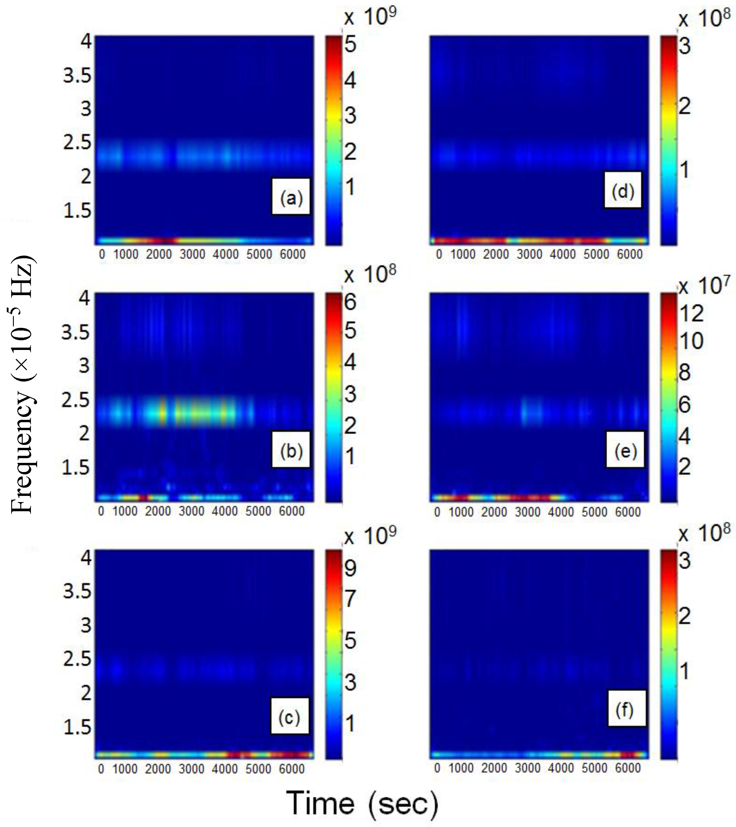
In order to make a quantitative comparison with the FFT results on power signals and to check whether taking into account also the non-stationary behavior can lead to different results, we have also used the complex Morlet wavelet mother as prototype of WT. For technical details about the basic formalism, see [25]. Note that this choice is not restrictive because other kinds of WT existing in literature would lead to very similar results. The calculated time-frequency behavior for both active and reactive powers is illustrated in Figure 3.

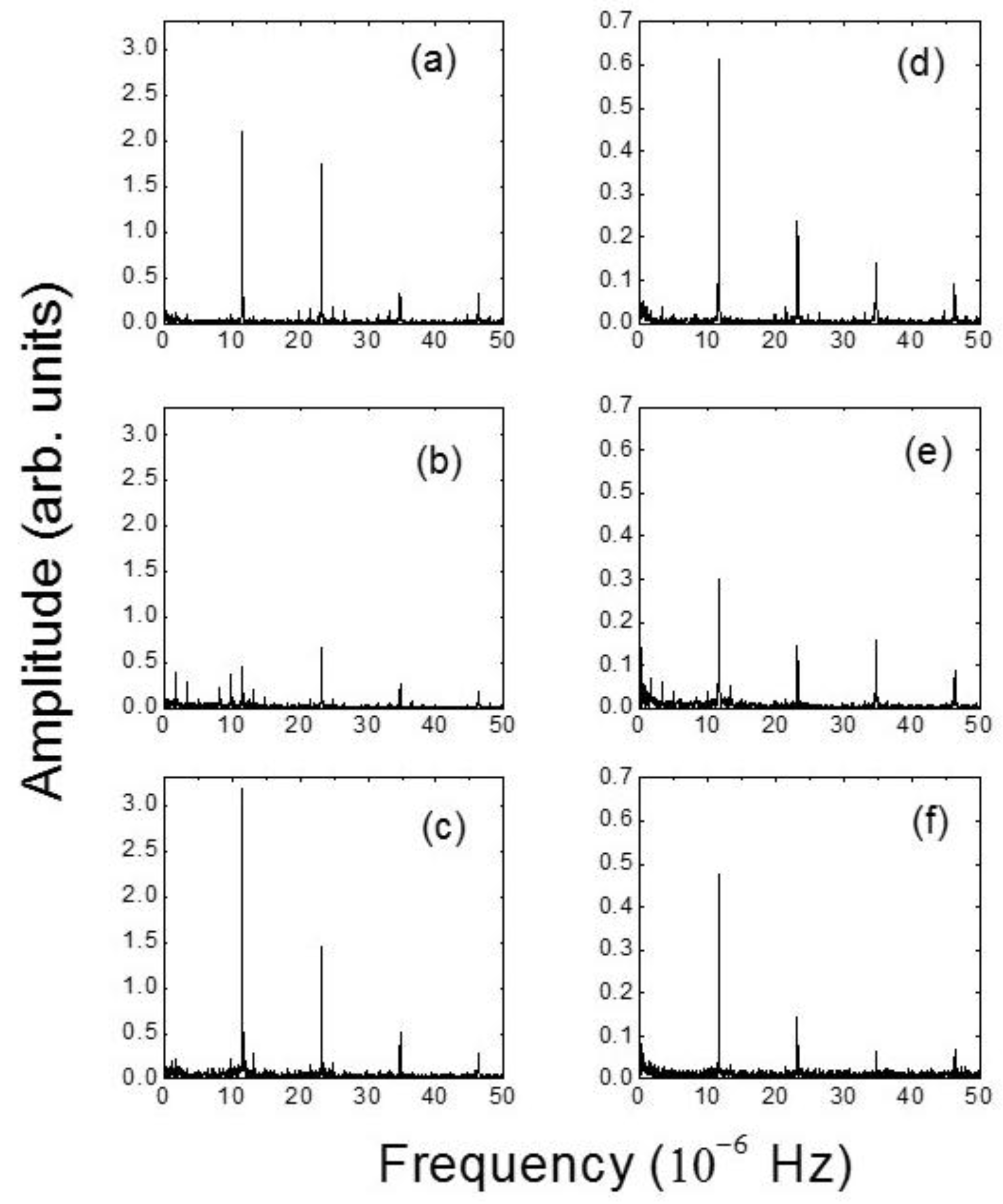
The frequencies extracted from the time-frequency domain are 11.55 × 10⁻⁶ Hz, 23.10 × 10⁻⁶ Hz, 34.70 × 10⁻⁶ Hz for the three lines. Looking at Figure 3 the two FFT frequencies corresponding to the harmonics H₁ and H₂ (24 h and 12 h, respectively) are found also according to the WT-based method both for active and reactive powers for lines L₁ and L₃, while for line L₂ only the one corresponding to 12 h was computed. Instead, the frequencies corresponding to the H₃ and H₄ harmonics (8 h and 6 h, respectively) lack in the WT analysis for the line L₃, but the frequency corresponding to H₃ compares well to the one found with WT analysis in lines L₁ (small value) and L₂. These results suggest that the non-stationary behavior included within the WT analysis does not lead to essential changes of the frequencies corresponding to the main H₁ and H₂ harmonics. On the other hand, a limited additional frequency present in the FFT spectra for the line L₂ corresponding to a week’s activity was also found.

Nevertheless, despite its solid basis, the above preliminary analysis performed according to the FFT and to the WT techniques does not allow the full characterization of the different lines―for instance, in terms of their non-linear behavior that is in turn strictly connected with the deviation from periodicity for an electrical power signal. For this reason, as a first further step the HHT analysis combined with the EMD has been applied to the three lines and the obtained results have been compared to the ones derived by means of the FFT and WT analysis. However, since the HHT-EMD tool did not completely quantitatively characterize the features of the power signal, the new suggested indices introduced in Section 2 have been computed. Note that the calculation of the three indices expressed in Equations (4)–(6) is the main step of our investigation.

4.3. HHT-EMD Results Compared to FFT and Wavelet Results: Calculation of Frequencies of IMFs

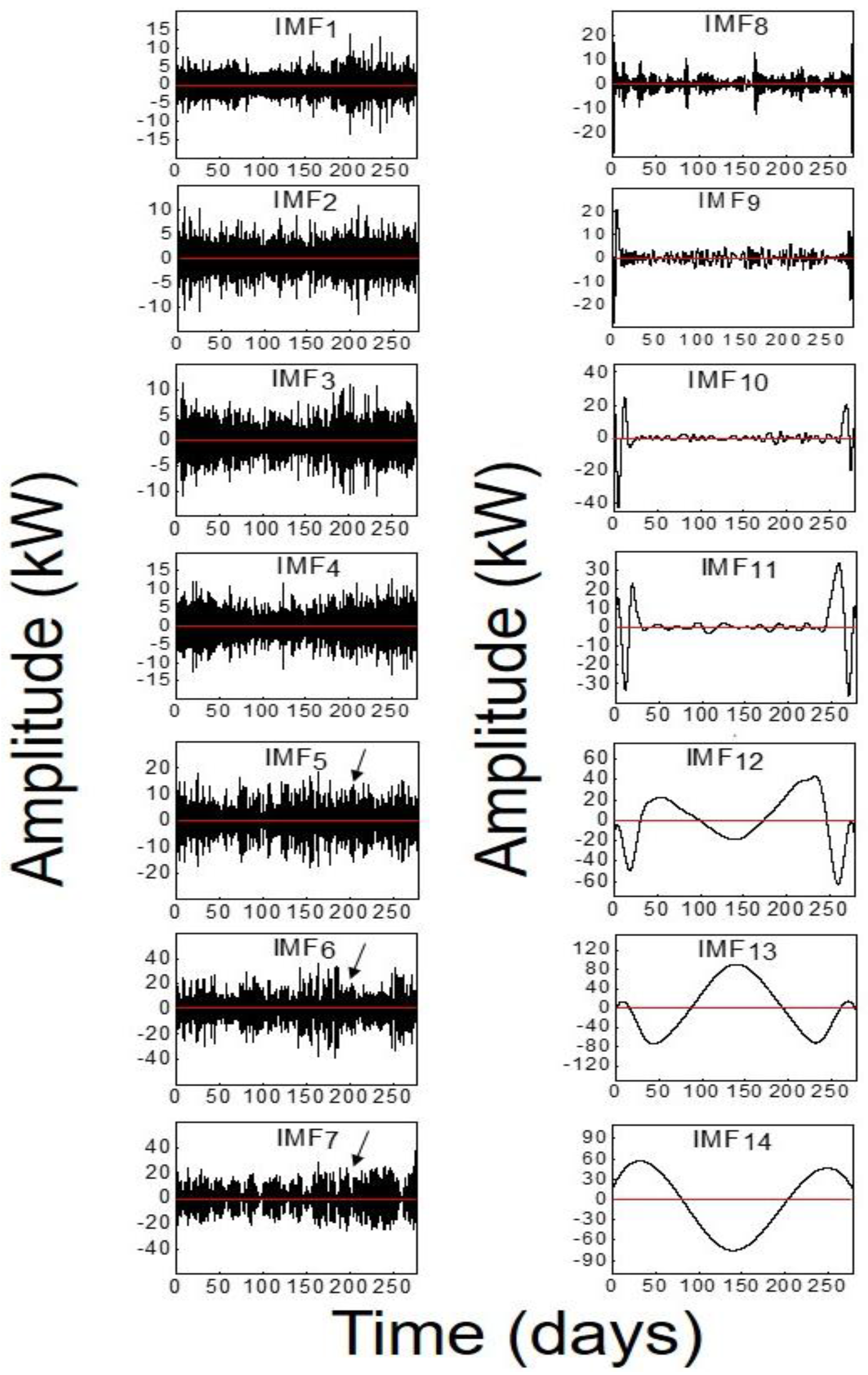
According to the EMD analysis based on the HHT technique, the electrical signal is decomposed into 14 IMFs for both the active and the reactive powers of the three lines. As an example, Figure 4 shows the time behavior of the 14 IMFs of the P₃ active power for the whole sampling period, labeled as IMF_i with I = 1, 2, … 14 in decreasing frequency order. The corresponding amplitudes of the IMFs related to the other active powers and reactive powers have a similar trend.

Looking at Figure 4, the number of oscillations of the IMFs decreases as the IMF order increases. This depends on the procedure used for the iterative extractions of each IMF. In fact, each step of EMD provides a new signal equal to the subtraction between the original one and the mean value of the envelope curves of its local maximum and minimum values. At the end of the process, it retains only the residual non-oscillatory term r_N (not shown).

Looking at the amplitudes of the IMFs it can be seen that there are no changes in the oscillation frequency, confirming that for each IMF amplitude there are no superpositions of different monocomponents. The IMFs 5–7 (denoted with arrows in Figure 4) have frequencies comparable to those corresponding to the FFT harmonics and also to some of the WT frequencies. The amplitudes averaged over the whole period have zero mean values, as should be expected.

The frequencies of the IMFs according to the average procedure described below are summarized in

Table 1. Frequencies of the 14 IMFs for L₁, L₂ and L₃ lines.

ν (×10−6 Hz)
P1	439.48	278.28	151.09	73.28	32.65	17.28	8.50	2.21	0.17	0.08	0.13	0.12	0.04	0.02
P2	440.85	283.98	156.79	82.73	43.01	22.75	11.82	5.16	1.29	0.79	0.46	0.12	0.08	0.04
P3	426.45	272.28	155.71	88.64	44.50	19.70	10.12	5.25	2.37	1.00	0.38	0.13	0.08	0.04
Q1	444.30	288.14	163.33	93.64	51.75	27.06	12.08	5.83	3.12	0.96	0.12	0.14	0.08	0.04
Q2	456.71	292.76	156.75	90.10	51.59	27.07	11.91	4.79	0.83	0.21	0.13	0.08	0.04	-
Q3	416.99	291.72	184.56	127.44	87.01	54.83	30.68	13.57	6.87	3.41	0.71	0.13	0.12	0.08

. As a general remark, it is evident that there is a greater number of frequencies calculated via the HHT-EMD than the ones determined by means of the FFT and WT analysis. This is not surprising because it is strictly connected mainly to the non-periodical behavior of the power signals in all the lines with different degrees of deviation from periodicity (see Section 4 for details) and to a lesser extent also to the non-stationary behavior. The deviation from a purely periodical behavior is in turn related to the non-linear behavior of power signals in DLs of SGs. In particular, the HHT approach combined with the EMD procedure allows the extraction of additional modes compared to the FFT.

Finally, just as EMD is based on the envelope curves of local maximum and minimum values, IMFs with lower frequencies can be extracted before IMFs with higher frequencies. For example, looking at the first row of Table 1 for P₁, it can be observed that IMF₁₀ has 0.08 × 10⁻⁶ Hz, whereas the IMF₁₁ and IMF₁₂ have higher frequencies, equal to 0.13 × 10⁻⁶ Hz and 0.12 × 10⁻⁶ Hz, respectively. Note that the frequencies shown in Table 1 are not properly the instantaneous frequencies expressed in Equation (3) that by definition depend on time as is typically shown in the so-called Hilbert spectrum. As a matter of fact, in order to compare the obtained frequencies with the corresponding ones computed via FFT and WT techniques, we have performed an average of the instantaneous IMF frequencies over the total sampling period. This procedure recalls the one employed for the calculation of the Hilbert average marginal spectrum obtained from the Hilbert spectrum by integrating it over the total sampling period and by dividing the result of this integration by the total sampling period. Of course, this analogy is no longer valid when the instantaneous frequency of the tone does not oscillate in a very narrow band so there could be points assigned to a different frequency in the Hilbert marginal spectrum. However, we would also like to stress that the Hilbert marginal spectrum has relevant meaning in the analysis of the HHT frequencies, is strictly connected to the HHT analysis and also used for extracting the general features of an electrical power signal. The advantage of this procedure is that it is possible to directly compare these mean single frequency values with the ones obtained with the other two techniques described above. On the other hand, this approach does not change the discussion since we have found that the instantaneous IMF frequencies extracted from the EMD technique do not appreciably vary with time despite the daily variations of loads in the different power lines. The weak variation as a function of time also characterizes the frequencies calculated by means of the WT analysis (see Figure 3).

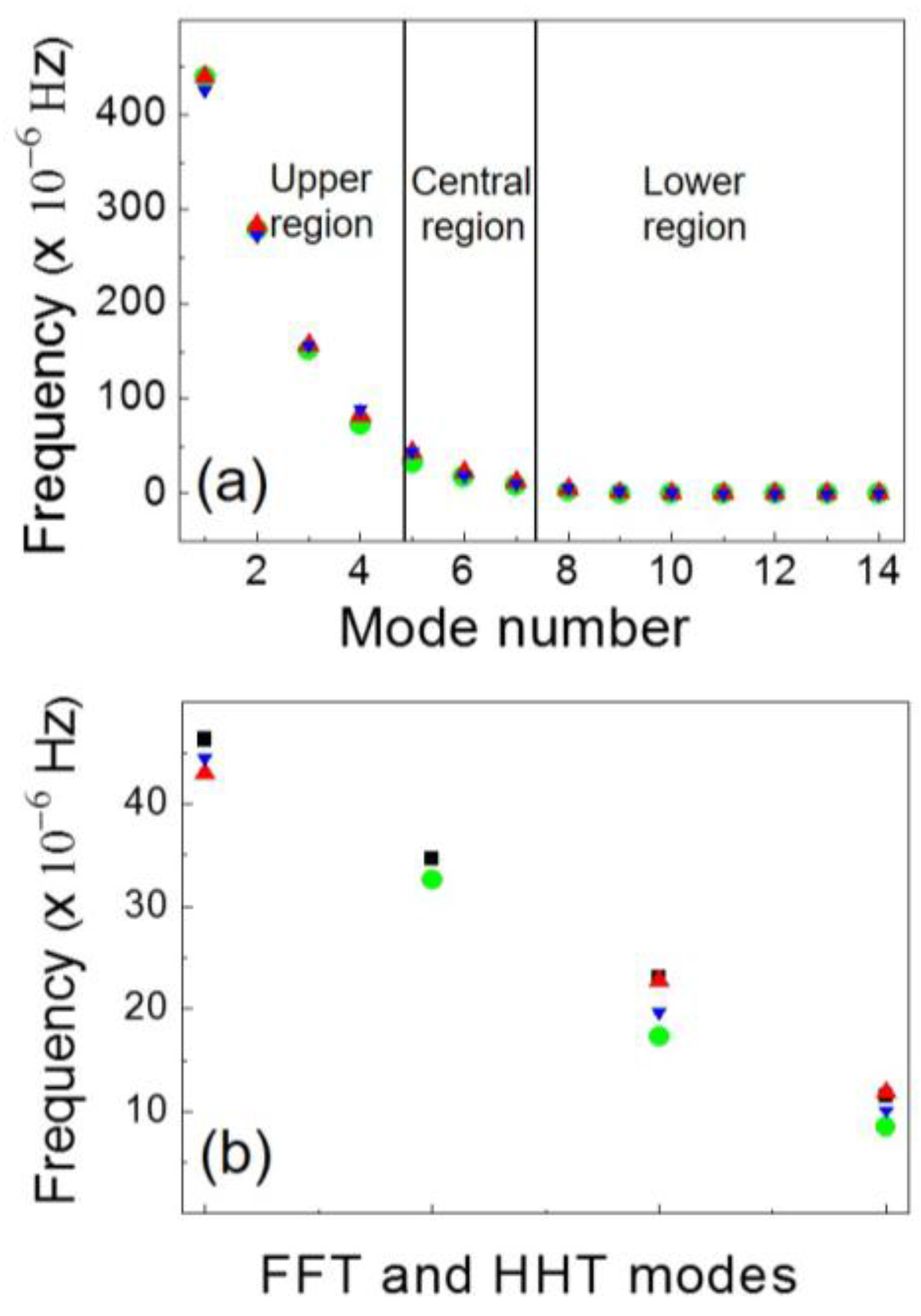
In order to clarify better the following discussion, we distinguish for every line three different frequency regions of the spectrum. In Figure 5a, the three frequency regions are shown by plotting the frequencies of the IMFs related to the three active powers. In addition to the central region, covering the frequency range of the typical harmonics found in the FFT spectrum, there are other two regions, the upper and the lower one. The lower region includes low frequencies with values up to about 5 × 10⁻⁶ Hz and, apart from one exception, the found frequencies are not present in the FFT spectrum. The central region has frequencies included in the range between about 10 × 10⁻⁶ Hz and about 50 × 10⁻⁶ Hz and corresponds more or less to the ones of the FFT spectrum. In the upper region there are frequencies having values above 50 × 10⁻⁶ Hz up to approximately 450 × 10⁻⁶ Hz; these frequencies are not present in the FFT spectrum. This wide range of frequencies computed via the HHT calculation is the combined result of the deviation from a purely periodical behavior, in turn strictly related to non-linearity effects that cannot be taken into account by the FFT analysis. For a detailed quantitative discussion on this point see next Section 4, where the calculated indices presented in Section 2 are discussed.

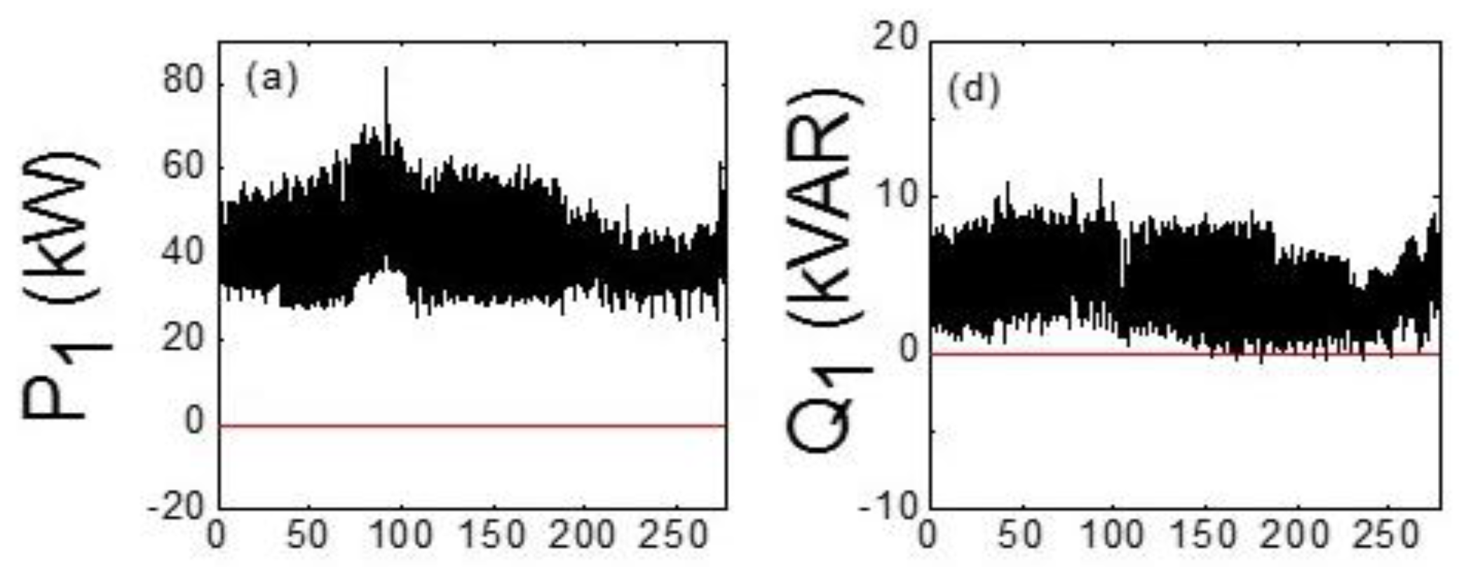
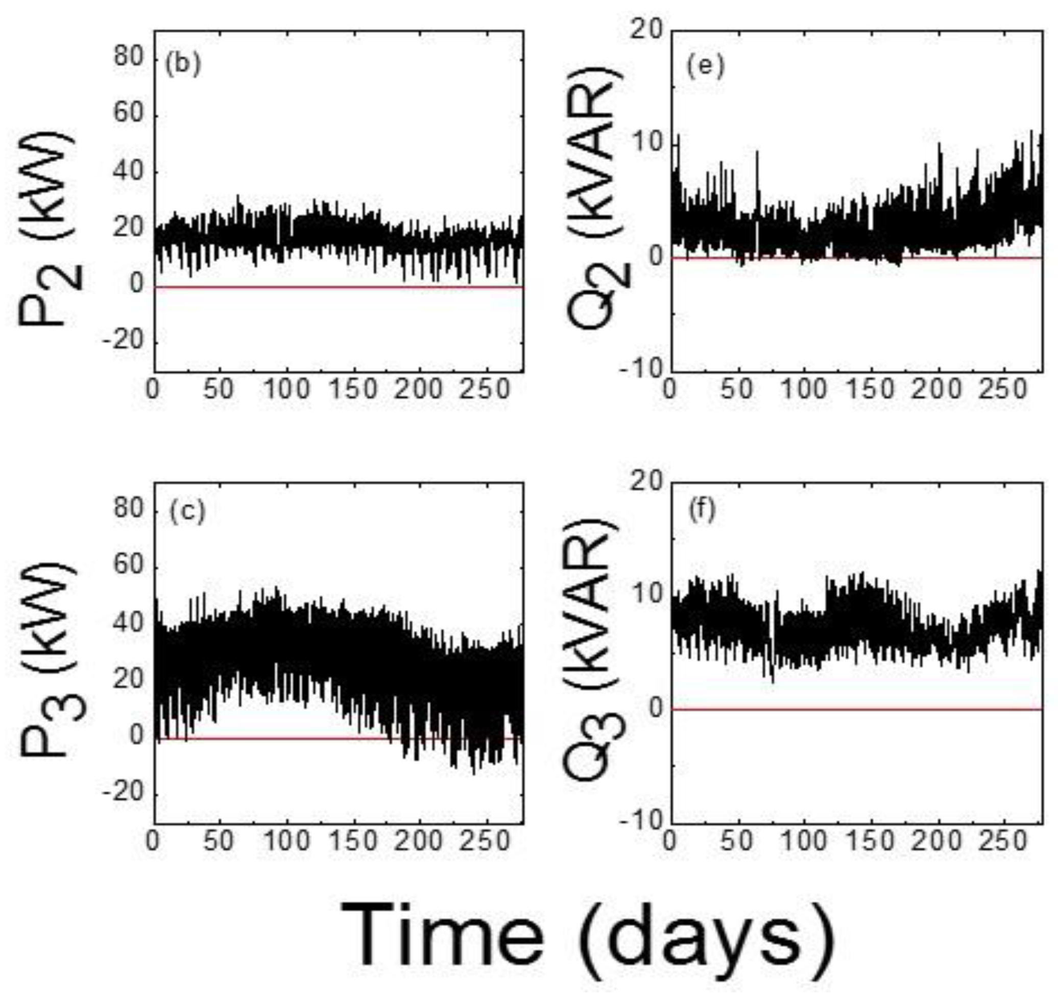
We now quantitatively discuss the frequencies related to the active powers. For the L₁ passive line and the L₃ active line the HHT frequencies differ appreciably especially in the upper and central regions (see also Table 1). This different trend is not surprising because of the strong difference in PV plants feeding the two lines which leads to different values of the active powers with P₃ assuming also negative values (see Figure 1c). Moreover, frequencies referred to the active powers of the L₂ passive line have overall different values with respect to those of P₁ and P₃.

More specifically, it is useful to make a quantitative comparison among the frequencies belonging to the central region with the corresponding frequencies of the typical FFT harmonics for P₁, P₂ and P₃ active powers. The comparison between the HHT-EMD frequencies and the FFT harmonics is illustrated in Figure 5b. For the first passive line L₁, the two first most representative frequencies 8.50 and 17.28 × 10⁻⁶ Hz (green circles) strongly differ from the frequencies of the H₁ (11.50 × 10⁻⁶ Hz) and H₂ (23.10 × 10⁻⁶ Hz) harmonics, respectively determined via the FFT (black squares), while the third one at 32.65 × 10⁻⁶ Hz has a much closer value to the frequency (34.70 × 10⁻⁶ Hz) of the H₃ harmonic.

On the other hand, there is no trace of the one corresponding to the 6 h peak as found according to the FFT. By contrast, the HHT-EMD frequencies corresponding to those of the H₁, H₂ and H₄ (46.30 × 10⁻⁶ Hz) harmonics for the second passive line L₂ (red up triangles) are rather close to the FFT ones, while the frequency related to the H₃ harmonic is not present in the HHT calculation. The frequencies obtained for the L₃ active line are slightly different with respect to the FFT ones especially those corresponding to the H₁ and H₂ harmonics (blue down triangles). Also for the L₃ active line there is the lack of the mode corresponding to the frequency of the H₃ harmonic and a frequency at 88.64 × 10⁻⁶ Hz not found according to the FFT calculation (it would be the equivalent of the frequency of the H₅ harmonic). This frequency corresponds to 3 h. The same conclusions can be drawn if the HHT-EMD frequencies are compared to the WT frequencies, which are superimposable to the ones of the FFT. Special attention deserves also the analysis of other characteristic frequencies belonging to the IMFs in the lower region of the spectrum. In particular, in addition to several frequencies not present in the FFT spectrum, the HHT analysis also confirms, for the L₂ passive line, the frequency (1.29 × 10⁻⁶ Hz) corresponding to 1 week found via the FFT analysis, which is typical of commercial loads. Concerning the frequencies of the IMFs above 50 × 10⁻⁶ Hz in the upper region, these would correspond approximately for every line to 2 h, 1 h and about ½ h, respectively. The above-mentioned additional features typical of the HHT spectrum and related to a combination of non-linear effects, deviation from a periodical behavior and non-stationary behavior were not extracted from the FFT and WT analysis.

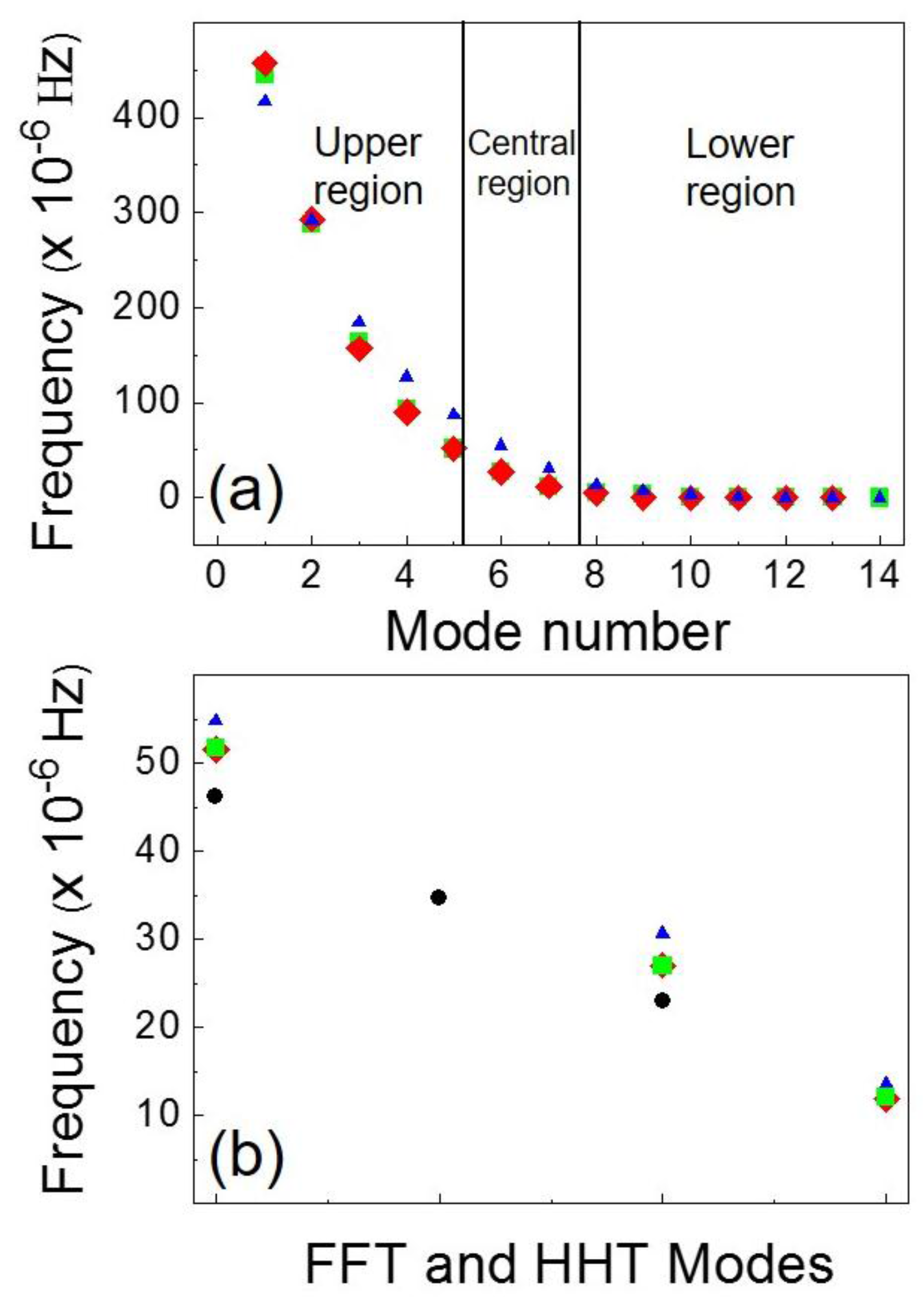
To check further the findings obtained for the P(t) signal we have processed the same datasets for the corresponding reactive powers Q(t) illustrated in Table 1 where the Q₂ reactive power has 13 IMFs frequencies and the Q₃ has 4 additional IMFs in the lower frequency region (not shown). The frequencies of the IMFs are also plotted in Figure 6a for Q(t) and subdivided into the three regions as done in Figure 5a. In Figure 6b the FFT frequencies of the main FFT harmonics related to the reactive powers are compared to the HHT corresponding ones in the central region of the spectrum.

Looking at Table 1 and Figure 6a, the frequencies of the IMFs corresponding to the Q₁ and Q₂ reactive powers are rather close each other due to the similar behavior of the signal (see Figure 1d,e), apart from some discrepancies which result from the difference between PV plants characterizing the L₁ and the L₂ passive lines. Instead, due to the different behavior of Q₃ (see Figure 1f), most of the calculated frequencies of the IMFs are different with respect to those of L₁ and L₂. Unlike the FFT analysis that gives very similar results, the comparison of the frequencies related to the active and the reactive powers, leads to different results. Indeed, there are significant differences between the frequencies related to the active powers and the corresponding ones associated to the reactive powers especially in the central region of the IMF frequencies. For example, the frequencies corresponding to those of the H₂ and H₃ harmonics typical of the FFT spectra were not found (see Figure 6b). The frequencies 12.08 × 10⁻⁶ Hz and 11.91 × 10⁻⁶ Hz rather close to that of the H₁ harmonic (11.50 × 10⁻⁶ Hz) were found only for Q₁ and Q₂ belonging to the lines L₁ and L₂, respectively but not for Q₃ belonging to the line L₃. Even though the HHT calculated frequencies 51.55 × 10⁻⁶ Hz, 51.72 × 10⁻⁶ Hz and 54.83 × 10⁻⁶ Hz for Q₁, Q₂ and Q₃ are higher than the frequency of the typical FFT H₄ harmonic (46.30 × 10⁻⁶ Hz), they can be considered their corresponding HHT frequencies. The found discrepancies can be ascribed to the more accurate analysis given by HHT.

In fact, the HHT computation is able to highlight the local properties of a typical power signal related to the effects of non-linearity that in turn give rise to its not-fully periodical character. In this respect, we believe that the deviation from periodicity of the power signal (for a quantitative analysis see Section 4) could lead to the lack of some of the frequencies in the HHT spectrum and especially the ones corresponding to the higher FFT harmonics.

We also performed an analysis of the data for single year’s quarters based on the HHT and some results are different (here not shown). For more details about this seasonal analysis see [34].

4.4. The Indices: Numerical Evaluation

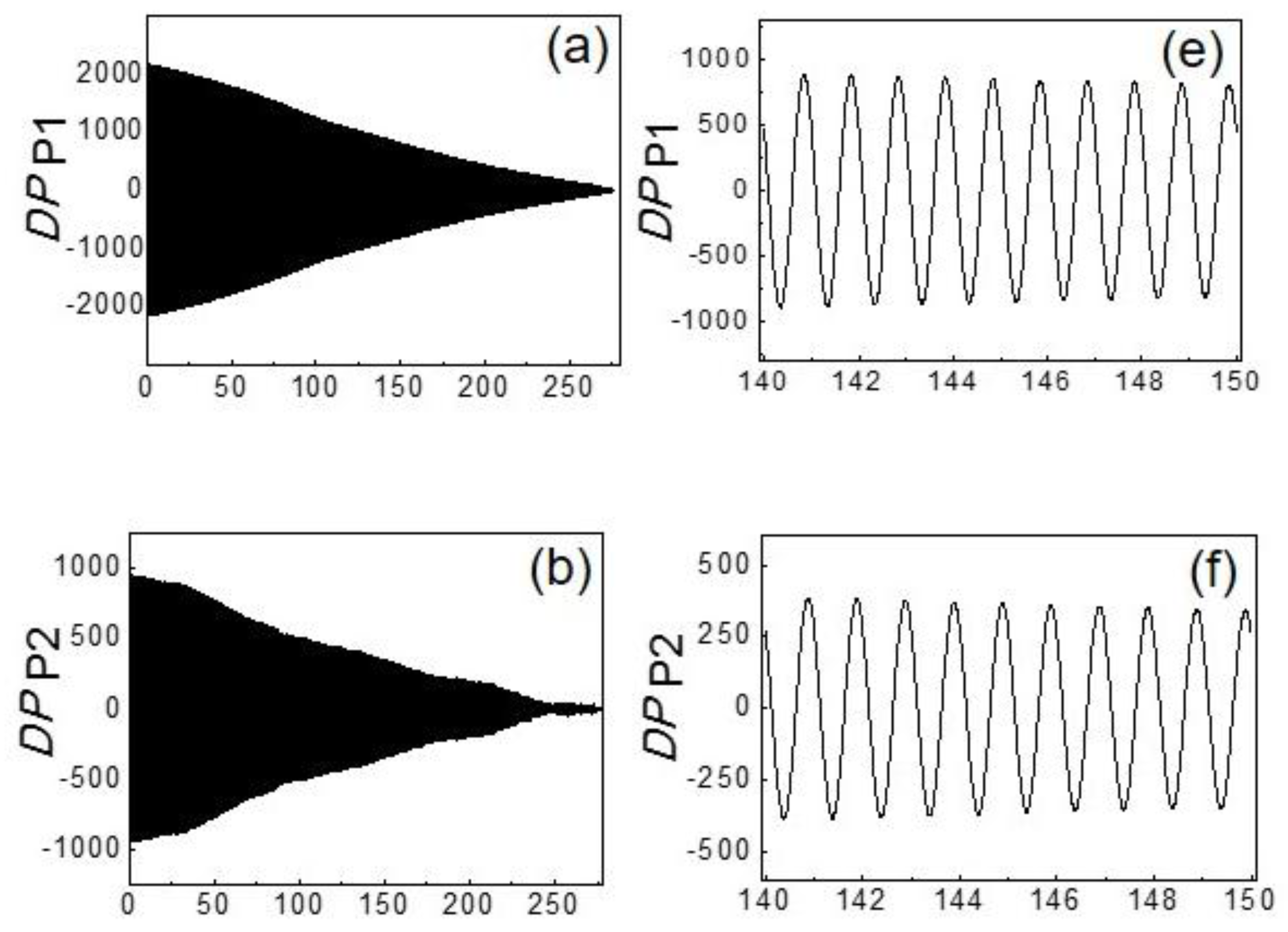
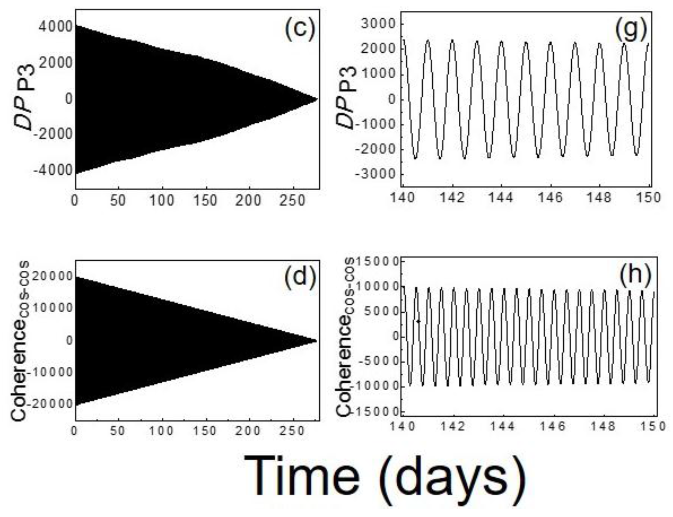
In this subsection, the results of the numerical computation of the indices expressed by Equations (4)–(6) are presented. In Figure 7 the DP index defined in Equation (4) and calculated for the P₁, P₂ and P₃ active powers is displayed, both for the total sampling period of 278 days in panels (a)–(c). In addition, a zoom of the signal for a temporal window ranging between the 140th and the 150th day (approximately located in the middle) is reported in panels (e)–(g) of Figure 6. As a reference, the coherence degree ${\text{Coherence}}_{\text{cos-cos}}$ as a function of time is displayed for a couple of cosine functions (see panel (d) and (h)). As expected, according to the definition of time-correlation functions [38], the general behavior is the decrease of the DP index amplitude with increasing time as illustrated in panels (a)–(d) marking a general reduction of the correlation of a given power signal with a cosine (or sine) function. From the analysis of the oscillation amplitudes, it turns out that the strongest deviation from the purely periodical behavior that is typical of a cosine (or sine) function having indeed the highest coherence degree characterizes the P₂ active power. This can be inferred by looking at the maximum oscillation amplitude of DP which for the P₂ active power is less pronounced (panel (f)) with respect to the ones involving the P₁ and P₃ active powers (panels (e) and (g)). In particular, in the shown temporal window of 10 days, the amplitude variation is about 750 for $D{P}_{{\mathrm{P}}_2}$, about 1700 for $D{P}_{{\mathrm{P}}_1}$ and more than 4000 for $D{P}_{{\mathrm{P}}_3}$. The oscillation amplitudes of $D{P}_{{\mathrm{P}}_1}$ and $D{P}_{{\mathrm{P}}_3}$ are much closer to the one characterizing the Coherence_cos-cos (panel (h)) between two cosine functions thus marking their higher periodicity degree. This behavior is very similar also by focusing on other temporal windows. The conclusions drawn for the DP index computed for the active powers remain valid also for the corresponding reactive powers. Therefore, the quantitative analysis on the DP index indicates that the L₁ passive line and the L₃ active line are characterized by a signal deviating to a lesser extent from the purely periodical behavior. First, from an overall analysis looking at Figure 7 it is important to note that the periodicity degree of the power signal does not strictly depend on the injected PV power, but it is strongly related to the loads and to the operating conditions. In particular, in this study we observe that the lines characterized by power signals with a smaller deviation from a purely periodical behavior are the ones feeding residential users, namely the L₁ passive line and the L₃ active line, one with no PV power and the other with a high PV power. However, from a more specific and deeper analysis it can be seen, by comparing panels (e), (g) and (h) of Figure 7, that the L₃ active line having the largest injected PV power is the one with the smaller deviation from a purely periodical behavior because it is characterized by the largest oscillation amplitudes. Therefore, the computation of the DP index could be helpful for highlighting the future advantages of planning lines having a high percentage of PV plants. Indeed, we can conclude that the more the concentration of PV plants is higher, the more the power signals tends towards periodical behavior, and this is potentially advantageous for the future operating conditions in DLs of SGs.

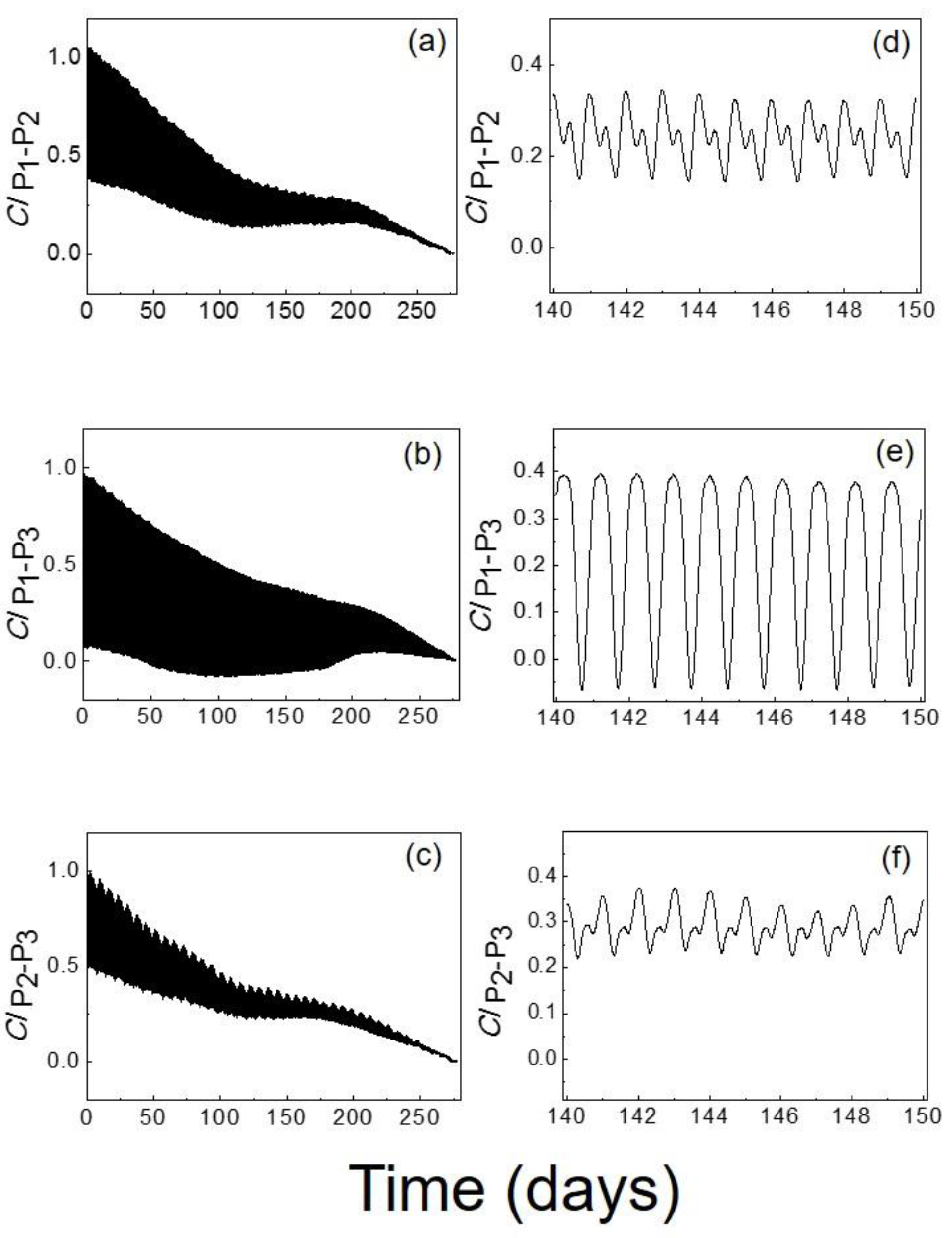
In Figure 8 the CI between a given couple of active powers defined in Equation (5) is shown in normalized units. According to its definition, resulting from the time-correlation function and similarly to the DP index also the amplitude of the CI reduces with increasing time. In panels (d)–(f) of Figure 7 the CI is shown in a temporal window ranging between the 140th and the 150th day. It can be noted that the CI trend as a function of time is strongly altered with an important amplitude reduction when the coherence is computed between the P₁ and P₂ and between the P₂ and P₃ active powers. Moreover, in this case there is also a reduced CI amplitude. Instead, $C{I}_{{\mathrm{P}}_1{-\text{P}}_3}$ exhibits regular oscillations marking a stronger coherence between the P₁ and P₃ active powers. The CI for the reactive powers shows very similar behavior with respect to that of the active powers, as occurred for the DP index. This can be understood by taking into account that the L₁ and L₃ lines feed residential users, while the L₂ line feeds commercial users. By means of this analysis we are able to quantify the coherence degree of two given power lines in different temporal windows and this can be done for any given available power line. As expected, the coherence degree resulting from the two residential lines, one active and the other passive, is higher than that computed between a residential line and a commercial line (one active and one passive or two passive lines).

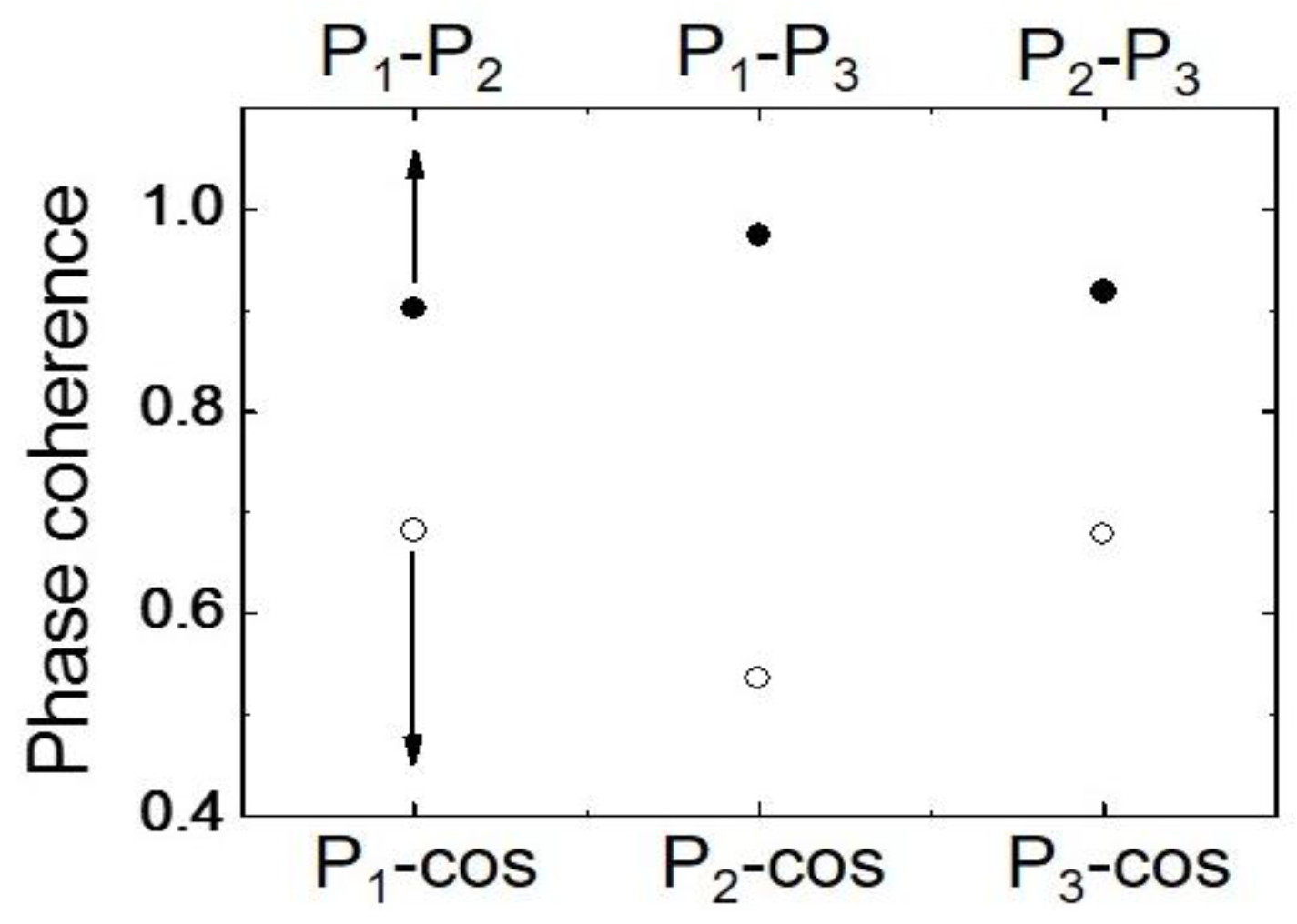
In order to validate the previous results the PC defined in Equation (6) has also been calculated. The results of this calculation are displayed in Figure 9. The phase coherence between the P₁, P₂ and P₃ active powers and the cosine function (empty circles) is higher for the two residential lines, being about 0.68 for P₁-cos and P₃-cos, while the one related to the commercial line (P₂-cos) is about 0.54.

These results show that the phase coherence with a co-sinusoidal (or sinusoidal) electrical signal is higher for the residential lines confirming the previous predictions. Moreover, the phase coherence between P₁ and P₃ (full circles) is equal to 0.97, while the ones between P₁ and P₂ and P₂ and P₃ active powers are about 0.90. According to this analysis, it can be established the PC for each given line and it is confirmed that the degree of phase coherence is higher between the two residential lines. Therefore, this index is useful to characterize the type of users of the line and it is not influenced by the quantity of installed PV power.

5. Conclusions

In summary, it has been shown that the HHT-EMD analysis applied to three different power lines belonging to an SG allows the extraction of several features that were not found according to the FFT and WT investigations, and the quantitative differences between the results obtained by means of the FFT, WT and HHT techniques have been discussed. The frequencies spectrum calculated via HHT-EMD is wider with respect to the ones found according to the FFT and WT analysis and this is mainly due to the non-periodical behavior of the electrical signals of power lines belonging to an SG in turn connected to their strong deviation from linearity.

An analysis giving important quantitative information about the features of power lines was carried out according to the calculation of new indices that are able to better characterize the electrical signal in terms of deviation from a purely periodical behavior and coherence properties. This is the key result of this study and completes the findings obtained by means of the previous analysis based on the usual mathematical tools. However, the indices proposed are defined according to a statistical approach starting from the electrical signals, and their information strongly differs from that given by the index of stationarity discussed in the literature.

It has been found that the higher the concentration of PV plants, the more the power signal tends towards a periodical behavior, and this can be an important advantage for planning the future operating conditions in DLs of SGs. Moreover, the power trend associated with the two residential lines has a higher periodicity degree than that of the commercial line. Finally, by computing the time and phase coherence indices it was also possible to establish in a quantitative way the coherence degree of two given power lines. Specifically, we have quantified the time and phase coherence degree correlating the lines having either more residential users or more commercial users. It was found that, in general, the time and phase coherence degree is higher between the two lines having more residential users. The proposed approach has helped to highlight the intrinsic features and the behavior of the power lines not evidenced by the study of the time signal according to the HHT-EMD analysis or by the simple application of the FFT and WT techniques. This approach, mainly focusing on the calculation of the proposed indices, can be usefully employed for the optimal operation and planning of SGs in the presence of strongly nonlinear loads and intermittent ones and it can be useful for the characterization of the lines with respect to the connected loads.

References

1. Farzanehrafat, A.; Watson, R. Power quality state estimator for smart distribution grids. IEEE Trans. Power Syst. 2013, 28, 2183–2191. [Google Scholar]
2. Smart Grid System Report, U.S. Department of Energy, August 2014. Available online: http://energy.gov/sites/prod/files/2014/08/f18/SmartGrid-SystemReport2014.pdf (accessed on 3 October 2015).
3. EPRI, Smart Grid Demonstration-Integration of Distributed Energy Resources. 2014. Available online: http://smartgrid.epri.com/Demo.aspx (accessed on 3 October 2015).
4. Tcheou, M.P.; Lovisolo, L.; Ribeiro, M.V.; da Silva, E.A.B.; Rodrigues, M.A.M.; Romano, J.M.T.; Diniz, P.S.R. The compression of electric signal waveforms for smart grids: State of the art and future trends. IEEE Trans. Smart Grid 2014, 5, 291–302. [Google Scholar]
5. Beyer, M.; Laney, D. The Importance of Big Data: A Definition; Gartner Research Report; Gartner: Stamford, CT, USA, 2012. [Google Scholar]
6. Ning, J.; Wang, J.; Gao, W.; Liu, C. A wavelet-based data compression technique for smart grid. IEEE Trans. Smart Grid 2011, 2, 212–218. [Google Scholar] [CrossRef]
7. IEEE Recommended Practice for Monitoring Electric Power Quality; IEEE Standard 1159-2009; IEEE: New York, NY, USA, 2009.
8. Huang, S.-J.; Jou, M.-J. Application of arithmetic coding for electric power disturbance data compression with wavelet packet enhancement. IEEE Trans. Power Syst. 2004, 19, 1334–1341. [Google Scholar]
9. Ribeiro, M.V.; Romano, J.M.T.; Duque, C.A. An improved method for signal processing and compression in power quality evaluation. IEEE Trans. Power Deliv. 2004, 19, 464–471. [Google Scholar]
10. Ribeiro, M.V.; Park, S.H.; Romano, J.M.T.; Mitra, S.K. A novel MDL-based compression method for power quality applications. IEEE Trans. Power Deliv. 2007, 22, 27–36. [Google Scholar] [CrossRef]
11. Vergura, S. Big data and efficiency of PV plants, IMEKO TC-4. In Proceedings of the International Symposium on Electrical Quantities, Benevento, Italy, 15–17 September 2014.
12. Eftekharnejad, S.; Vittal, V.; Heydt, G.T.; Keel, B.; Loehr, J. Impact of increased penetration of photovoltaic generation on power systems. IEEE Trans. Power Syst. 2013, 28, 893–901. [Google Scholar] [CrossRef]
13. Du, W.; Wang, H.F.; Dunn, R. Power system small-signal oscillation stability as affected by large-scale PV penetration. International Conference on Sustainable Power Generation and Supply 2009, 1–4, 1684–1689. [Google Scholar]
14. Gopakumar, P.; Jaya Bharata Reddy, M.; Kumar Mohanta, D. Stability concerns in smart grid with emerging renewable energy technologies. Int. J. Electr. Power Compon. Syst. 2014, 42, 418–425. [Google Scholar] [CrossRef]
15. Cecati, C.; Citro, C.; Siano, P. Combined operations of renewable energy systems and responsive demand in a smart Grid. IEEE Trans. Sustain. Energy 2011, 2, 468–476. [Google Scholar] [CrossRef]
16. Guo, Y.; Li, C.; Li, Y.; Gao, S. Research on the power system fault classification based on HHT and SVM using wide-area information. Energy Power Eng. 2013, 5, 138–142. [Google Scholar] [CrossRef]
17. Senroy, N.; Suryanarayanan, S.; Ribeiro, P.F. An improved Hilbert-Huang method for analysis of time-varying waveforms in power quality. IEEE Trans. Power Syst. 2007, 22, 1843–1850. [Google Scholar] [CrossRef]
18. Mehta, K.; Russell, B.D. Data compression for digital data from power systems disturbances: Requirements and technique evaluation. IEEE Trans. Power Deliv. 1989, 4, 1683–1688. [Google Scholar] [CrossRef]
19. Gerek, O.N.; Ece, D.G. Compression of power quality event data using 2D representation. Electr. Power Syst. Res. 2008, 78, 1047–1052. [Google Scholar]
20. Kraus, J.; Tobiska, T.; Bubla, V. Looseless encodings and compression algorithms applied on power quality datasets. In Proceedings of the 20th International Conference and Exhibition on Electricity Distribution—Part 1, Prague, Czech Republic, 8–11 June 2009; pp. 1–4.
21. Kraus, J.; Stepan, P.; Kukacka, L. Optimal data compression techniques for smart grid and power quality trend data. In Proceedings of the 15th International Conference on Harmonics and Quality of Power (ICHQP), Hong Kong, China, 17–20 June 2012; pp. 707–712.
22. Qing, A.; Hongtao, Z.; Zhikun, H.; Zhiwen, C. A compression approach of power quality monitoring data based on two-dimension dct. In Proceedings of the 2011 Third International Conference on Measuring Technology and Mechatronics Automation (ICMTMA), Shanghai, China, 6–7 January 2011; pp. 20–24.
23. Tse, N.C.F.; Chan, J.Y.C.; Lai, L.L. Development of a smart metering scheme for building smart grid system. In Proceedings of the 8th International Conference on Advances in Power System Control, Operation and Management (APSCOM 2009), Hong Kong, China, 8–11 November 2009; pp. 1–5.
24. Zhang, M.; Li, K.; Hu, Y. A high efficient compression method for power quality applications. IEEE Trans. Instrum. Meas. 2011, 60, 1976–1985. [Google Scholar] [CrossRef]
25. Vergura, S.; Siracusano, G.; Carpentieri, M.; Finocchio, G. A nonlinear and non-stationary signal analysis for accurate power quality monitoring in smart grids. In Proceedings of the 3rd Renewable Power Generation Conference (IET-RPG), Naples, Italy, 24–25 September 2014; pp. 1–6.
26. Huang, N.E.; Shen, Z.; Long, S.R.; Wu, M.C.; Shih, H.H.; Zheng, Q.; Yen, N.-C.; Tung, C.C.; Liu, H.H. The empirical mode decomposition and the Hilbert spectrum for nonlinear and non-stationary time series analysis. Proc. R. Soc. Lond. A 1998, 454, 903–995. [Google Scholar] [CrossRef]
27. Oberlin, T.; Meignen, S.; Perrier, V. An alternative formulation for the empirical mode decomposition. IEEE Trans. Signal Process. 2012, 60, 2236–2246. [Google Scholar] [CrossRef]
28. Coughlin, K.; Tung, K. 11-year solar cycle in the stratosphere extracted by the empirical mode decomposition method. Adv. Space Res. 2004, 34, 323–329. [Google Scholar] [CrossRef]
29. Peng, S.; Hwang, W. Adaptive signal decomposition based on local narrow band signals. IEEE Trans. Signal Process. 2008, 56, 2669–2676. [Google Scholar] [CrossRef]
30. Mandic, D.P.; Rehman, N.U.; Wu, Z.; Huang, N.E. Empirical mode decomposition-based time-frequency analysis of multivariate signals. IEEE Signal Process. Mag. 2013, 30, 74–86. [Google Scholar] [CrossRef]
31. Huang, N.E.; Kunot, A. An optimization based EMD scheme. J. Comput. Appl. Math. 2013, 240, 174–183. [Google Scholar] [CrossRef]
32. Wang, T.; Zhang, M.; Yu, Q.; Zhang, H. Comparing the applications of EMD and EEMD on time-frequency analysis of seismic signal. J. Appl. Geophys. 2012, 83, 29–34. [Google Scholar] [CrossRef]
33. Vergura, S.; Acciani, G.; Amoruso, V.; Patrono, G.E.; Vacca, F. Descriptive and inferential statistics for supervising and monitoring the operation of PV plants. IEEE Trans. Ind. Electron. 2009, 56, 4456–4464. [Google Scholar] [CrossRef]
34. Vergura, S.; Zivieri, R.; Carpentieri, M. Seasonal signal analysis of distribution lines in smart grids via hilbert-huang transform. In Proceedings of the 15th International Conference on Environment and Electrical Engineering (EEEIC), Roma, Italy, 10–13 June 2015; pp. 1420–1425.
35. Huang, N.E.; Attoh-Okine, N.O. The Hilbert-Huang Transform in Engineering; CRC Press: London, UK, 2005. [Google Scholar]
36. Laurent, H.; Doncarli, C. Stationary index for abrupt changes detection in the time-frequency plane. IEEE Signal Process. Lett. 1998, 5, 43–45. [Google Scholar] [CrossRef]
37. Huang, N.E.; Wu, Z.; Long, S.R.; Arnold, K.C.; Chen, X.; Blank, K. On instantaneous frequency. Adv. Adapt. Data Anal. 2009, 1, 177–229. [Google Scholar] [CrossRef]
38. Zivieri, R.; Santoro, G.; Bortolani, V. Anharmonicity on Al(100) and Al(111) surfaces. Phys. Rev. B 1999, 59, 15959–15965. [Google Scholar] [CrossRef]
39. Carpentieri, M.; Torres, L.; Martinez, E. Temperature dependence of microwave nano-oscillator linewidths driven by spin-polarized currents: A micromagnetic analysis. IEEE Trans. Magn. 2009, 45, 3426–3429. [Google Scholar] [CrossRef]
Figure 1. (a) Active power P1; (b) active power P2; (c) active power P3; (d) reactive power Q1; (e) reactive power Q2; and (f) reactive power Q3.
Energies 09 00211 g001aEnergies 09 00211 g001b
Figure 2. FFT spectra. (a) FFT of the P1 active power; (b) FFT of the P2 active power; (c) FFT of the P3 active power; (d) FFT of the Q1 reactive power; (e) FFT of the Q2 reactive power and (f) FFT of the Q3 reactive power.
Energies 09 00211 g002
Figure 3. Time-frequency domain plot computed according to the WT-based method. (a) WT of the P1 active power; (b) WT of the P2 active power; (c) WT of the P3 active power; (d) WT of the Q1 reactive power; (e) WT of the Q2 reactive power and (f) WT of the Q3 reactive power.
Energies 09 00211 g003
Figure 4. Amplitude of the 14 IMFs as a function of time related to the P3 active power. An arrow indicates the amplitudes of the IMFs having frequencies close to the ones of the harmonics obtained via the FFT analysis (see the text for a discussion).
Energies 09 00211 g004
Figure 5. (a) HHT-EMD frequencies for the active power P of L1, L2 and L3 subdivided into the three frequency regions (upper, central and lower) of the HHT spectrum. Green circles: HHT frequencies for P1. Red up triangles: HHT frequencies for P2. Blue down triangles: HHT-EMD frequencies for P3; (b) main FFT frequencies compared to the HHT-EMD frequencies of the central region for the active power of L1, L2 and L3. Black squares: FFT harmonics H1, H2, H3 and H4. The meaning of the other symbols is the same as in panel (a).
Energies 09 00211 g005
Figure 6. (a) HHT-EMD frequencies for the reactive power of L1, L2 and L3 subdivided into the three frequency regions (upper, central and lower) of the HHT spectrum. Green squares: HHT frequencies for Q1. Red diamonds: HHT-EMD frequencies for Q2. Blue up triangles: HHT frequencies for Q3. (b) Main FFT frequencies compared to the HHT-EMD frequencies of the central region for the reactive power of L1, L2 and L3. Black circles: FFT harmonics H1, H2, H3 and H4. The meaning of the other symbols is the same as in panel (a).
Energies 09 00211 g006
Figure 7. DP index for the three active powers and for the cosine function. (a) D P P 1 ; (b) D P P 2 ; (c) DPP3; (e) DPP1 in a temporal window; (f) DPP2 in a temporal window; (g) D P P 3 in a temporal window; (d) Coherence cos-cos and (h) Coherence cos-cos in a temporal window.
Energies 09 00211 g007aEnergies 09 00211 g007b
Figure 8. CI between couples of active powers. (a) C I P 1 P 2 ; (b) C I P 1 P 3 ; (c) C I P 2 P 3 ; (d) C I P 1 P 2 in a temporal window; (e) C I P 1 P 3 in a temporal window; and (f) C I P 2 P 3 in a temporal window.
Energies 09 00211 g008
Figure 9. PC between couples of active powers (full circles) and between a given active power and the cosine function (empty circles).
Energies 09 00211 g009