SVM-Based Multiple Instance Classification via DC Optimization
by
 , and
, and
Annabella Astorino
1,*,† ,
,
Antonio Fuduli
2,†,
Giovanni Giallombardo
3,† and
Giovanna Miglionico
3,† 1
Istituto di Calcolo e Reti ad Alte Prestazioni-C.N.R., 87036 Rende (CS), Italy
2
Dipartimento di Matematica e Informatica, Università della Calabria, 87036 Rende (CS), Italy
3
Dipartimento di Ingegneria Informatica, Modellistica, Elettronica e Sistemistica, Università della Calabria, 87036 Rende (CS), Italy
*
Author to whom correspondence should be addressed.
†
These authors contributed equally to this work.
Algorithms 2019, 12(12), 249; https://0-doi-org.brum.beds.ac.uk/10.3390/a12120249
Submission received: 31 October 2019
/
Revised: 19 November 2019
/
Accepted: 20 November 2019
/
Published: 23 November 2019
(This article belongs to the Special Issue Nonsmooth Optimization in Honor of the 60th Birthday of Adil M. Bagirov)
Abstract
:A multiple instance learning problem consists of categorizing objects, each represented as a set (bag) of points. Unlike the supervised classification paradigm, where each point of the training set is labeled, the labels are only associated with bags, while the labels of the points inside the bags are unknown. We focus on the binary classification case, where the objective is to discriminate between positive and negative bags using a separating surface. Adopting a support vector machine setting at the training level, the problem of minimizing the classification-error function can be formulated as a nonconvex nonsmooth unconstrained program. We propose a difference-of-convex (DC) decomposition of the nonconvex function, which we face using an appropriate nonsmooth DC algorithm. Some of the numerical results on benchmark data sets are reported.
1. Introduction
Multiple instance learning (MIL) is a recent machine learning paradigm [1,2,3], which consists of classifying sets of points. Each set is called bag, while the points inside the bags are called instances. The main characteristic of an MIL problem is that in the learning phase the instance labels are hidden and only the labels of the bags are known.
An MIL seminal paper is [4], where a drug-design problem has been faced. Such a problem consists of determining whether a drug molecule (bag) is active or non-active. A molecule provides the desired drug effect (positive label) if, and only if, at least one of its conformations (instances) binds to the target site. The crucial question is that it is not known a priori which conformation makes the molecule active.
Some MIL applications are image classification [5,6,7,8], drug discovery [9,10], classification of text documents [11], bankruptcy prediction [12], and speaker identification [13].
For this kind of problems, there are various solutions in the literature that fall into three different classes: instance-space approaches, bag-space approaches, and embedding-space approaches. In instance-space approaches, classification is performed at the instance level, finding a separation surface directly in the instance space, without looking at the global structure of the bags; the label of each bag is determined as an aggregation of the labels of its corresponding instances. Vice-versa, in bag-space approaches (for example, see [14,15,16]), the separation is performed at a global level, considering the bag as a whole entity. A compromise between these two kinds of approaches is constituted by embedding-space techniques, where each bag is represented by one feature vector and the classification is consequently performed in the instance space. An example of an embedding-space approach is presented in [17].
The method we propose uses the instance-space approach and provides a separation hyperplane for the binary case, where the objective is to discriminate between positive and negative bags. We start from the standard MIL assumption stating that a bag is positive if, and only if, at least one of its instances is positive and it is negative whenever all its instances are negative.
Some examples of linear instance-space MIL classifiers can be found in [18,19,20,21,22]. In particular, in [18], two different models have been proposed. The first one is a mixed-integer nonlinear optimization problem solved using a heuristic technique based on the block coordinate descent method [23] and faced in [19] using a Lagrangian relaxation technique. The second model, which will be the objective of our analysis in the next section, is a nonsmooth nonconvex optimization problem, solved in [21] using the bundle type method described in [24]. In [20], a semi-proximal support vector machine (SVM) approach is used, coming from a compromise between the classical SVM [25] and the proximal approach proposed in [26] for supervised classification. Finally, an optimization problem with bilinear constraints is analyzed in [22], where each positive bag is expressed as a convex combination of its instances and a local solution is obtained by solving successive linear programs.
Recently, nonlinear instance-space MIL classifiers have also been proposed in the literature, such as in [27] and in [28], where a spherical separation approach is adopted: in particular, in the former a variable neighborhood search method [29] is used, while in the latter a DC (difference of convex) model is solved using an appropriate DC algorithm [30]. In passing, we stress that many DC models have been introduced in machine learning, in the supervised [31,32,33,34,35], semisupervised [36,37] and unsupervised cases [38,39,40].
In this work, we propose a DC optimization model providing a linear classifier for binary MIL problems. The solution method we adopt is the proximal bundle method introduced in [30] for the minimization of nonsmooth DC functions. The paper is organized as follows. In the next two sections, we describe, respectively, the DC optimization model and the corresponding nonsmooth solution algorithm. Finally, in Section 4, we report the results of our numerical experimentation performed on some data sets drawn from the literature.
2. A DC Decomposition of the SVM-Based MIL
We tackle a binary MIL problem whose objective is to discriminate between m positive bags and k negative ones using a hyperplane
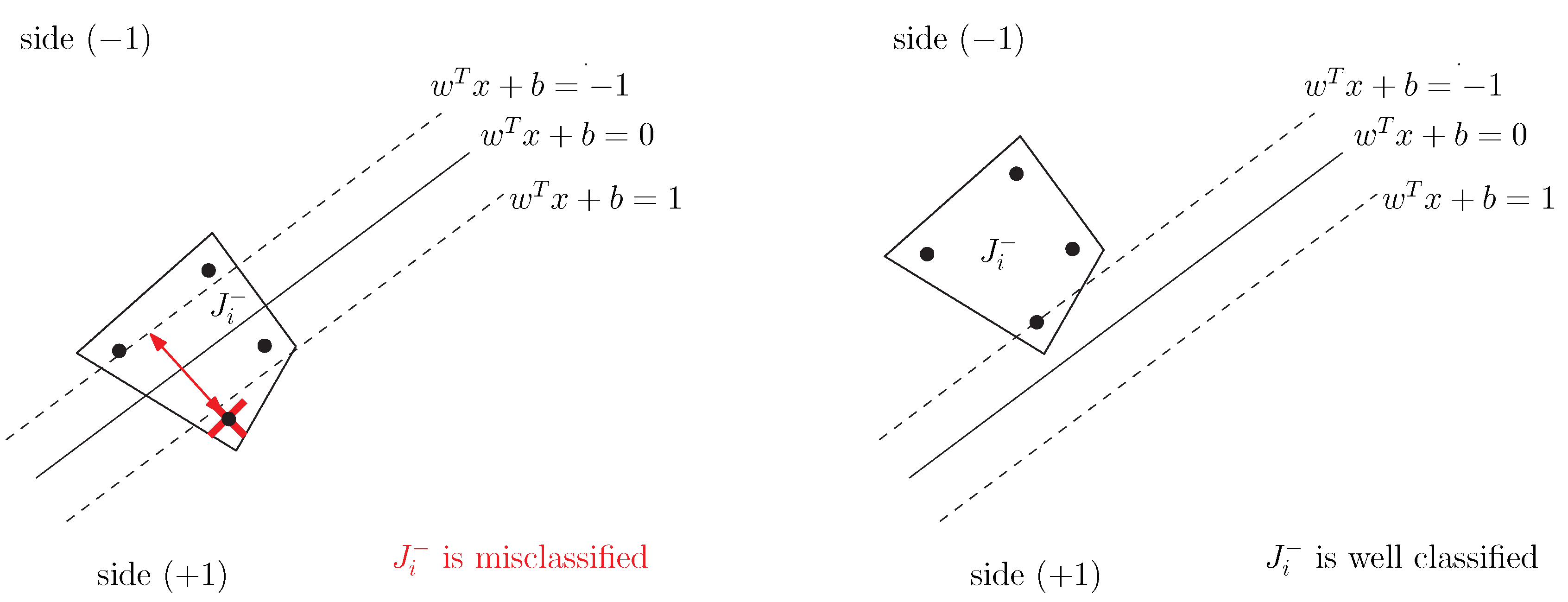
where and . Indicating by , , the index set of the instances belonging to the ith positive bag and by , , the index set of the instances belonging to the ith negative bag, we recall that, on the basis of the standard MIL assumption, a bag is positive if, and only if, at least one of its instances is positive and it is negative vice-versa. As a consequence, while a positive bag is allowed to, possibly, straddle the hyperplane, the negative bags should lie completely on the negative side.
More formally, indicating by the jth instance of a positive or negative bag, the hyperplane performs a correct separation if, and only if, the following conditions hold:
As a consequence (see Figure 1 and Figure 2), a positive bag , , is misclassified if
and a negative one , , is misclassified if
Then, we come out with the following error function, already introduced in [18]:
where represents the trade-off between two objectives: the maximization of the separation margin, characterizing the classical SVM [25] approach, and the minimization of the classification error.
To minimize function f, we propose a DC decomposition based on the following formula:
where h is a convex function. By applying Equation (2) to our case, we can write f in the form:
where
and
are convex functions. Hence, we come up with the following nonconvex nonsmooth optimization problem, DC-MIL,
3. Solving DC-MIL Using a Nonsmooth DC Algorithm
We start by recalling some preliminary property of the DC optimization problem, by adopting the same notation as above. Given the DC optimization problem
where both and are convex nonsmooth functions, we say that a point is a local minimizer if is finite and there exists a neighborhood of such that
Considering that, in general, the Clarke subdifferential calculus cannot be used to compute subgradients of the DC function since
where denotes Clarke’s subdifferential, different stationary points can be defined for nonsmooth DC functions. A point is called inf-stationary for problem Equation (4) if
Furthermore, a point is called Clarke stationary for problem Equation (4) if
while, it is called a critical point of f if
Denoting the set of inf-stationary points by , the set of Clarke stationary points by , and the set of critical points of the function f by , the following inclusions hold
as shown in (Proposition 3, [30]).
Nonsmooth DC functions have attracted the interest of several researchers, both, from the theoretical and from the algorithmic viewpoint. Focusing in particular on the algorithmic side, the most relevant contribution has probably been provided by the methods based on the linearization of function (see, [41] and references therein), where the problem is tackled via successive convexifications of function f. In the last years, nonsmooth-tailored DC programming has experienced a lot of attention as it has a lot of practical applications (see [28,42]). In fact, several nonsmooth DC algorithms have been developed ([30,43,44,45,46,47]).
Here, we adopt the algorithm DCPCA, a bundle-type method introduced in [30] to solve problem Equation (4), which is based on a model function built by combining two convex piecewise approximations, each related to one component function. More in details, a simplified version of DCPCA works as follows:
- It iteratively builds two separate piecewise-affine approximations of the component functions, grouping the corresponding information in two separate bundles.
- It combines the two convex piecewise-affine approximations and generates a DC piecewise-affine model.
- The DC (hence, nonconvex) model is locally approximated using an auxiliary quadratic program, whose solution is used to certify approximate criticality, or to generate a descent search-direction to be explored via a backtracking line-search approach.
- Whenever no descent is achieved along the search direction, the bundle of the first function is enriched, thus, obtaining a better model function with this being the fundamental feature of any cutting plane algorithm.
In fact, the DCPCA is based on constructing a model function as the pointwise maximum of several concave piecewise-affine pieces. To construct this model, starting from some cutting-plane ideas, the information coming from the two component functions are kept separate in two bundles. We denote the stability center by z (i.e., an estimate of the minimizer), and by I and L, the index sets of the points generated by the algorithm where the information of function and have been evaluated, respectively. Therefore, we denote the two bundles of information as
and
where, for every , with
and, for every , with
We remark that both component functions, along with their subgradients, could be evaluated at some iterate-point, and, indeed, we assume that and , where and .
To approximate the difference function
at a given iteration k the following nonconvex model function is introduced
which is defined as the maximum of finitely many concave piecewise-affine functions. The model- function is used to state a sufficient descent condition of the type
where . The interesting property of such a model-function is that whenever the sufficient descent is not achieved at points that are close to the stability center, say , then an improved cutting-plane model can be obtained by only updating the bundle of with the appropriate information related to the point . On the other hand, it looks obviously difficult to adopt the minimization of the model-function as a building block of any algorithm, given its nonconvexity. In fact, DCPCA does not require the direct minimization of , but the search direction can be obtained by solving the following auxiliary quadratic problem:
where . We observe that as is assumed to contain the information about the current stability center. More precisely, DCPCA works by forcing to be a singleton, hence by letting . Denoting the unique optimal solution of Equation (QP(I)) by , a standard duality argument ensures that
where , , are the optimal variables of the dual of , with .
Given that any starting point , DCPCA returns an approximate critical point , see (Theorem 1, [30]). The following parameters are adopted: the optimality parameter , the subgradient threshold , the linearization-error threshold , the approximate line-search parameter , and the step-size reduction parameter . In Algorithm 1, we report an algorithmic scheme of the main iteration, namely of the set of steps where the stability center is unchanged. An exit from the main iteration is obtained as soon as a stopping criterion is satisfied or whenever the stability center is updated. To make the presentation clearer, without impairing convergence properties, we skip the description of some rather technical steps, which are strictly related to the management of bundle . Details can be found in [30].
| Algorithm 1 DCPCA Main Iteration | |
| 1: Solve QP(I) and obtain | ▹ Find the search-direction and the predicted-reduction |
| 2: if then | ▹ Stopping test |
| 3: set and exit | ▹ Return the approximate critical point |
| 4: end if | |
| 5: Set | ▹ Start the line-search |
| 6: if then | ▹ Descent test |
| 7: set | ▹ Make a serious step |
| 8: calculate and | ▹ | |
| 9: update for all and for all | ▹ | |
| 10: set | ▹ | |
| 11: set | ▹ | |
| 12: update appropriately I and L, and go to 1 | ▹ | |
| 13: else if then | ▹ Closeness test |
| 14: set and go to 6 | ▹ Reduce the step-size and iterate the line-search |
| 15: end if | |
| 16: Calculate | ▹ Make a null step |
| 17: calculate | ▹ | |
| 18: set , update appropriately I, and go to 1 | ▹ | |
We remark that the stopping condition , checked at Step 2 of the DCPCA, is an approximate -criticality condition for . Indeed, taking into account Equation (12), the stopping condition ensures that
which in turn implies that and such that
namely, that
an approximate -criticality condition for , see Equation (9).
4. Results
We tested the performance of the algorithm DCPCA applied to the DC-MIL formulation (3) by adopting two sets of medium- and large-size problems extracted from [18]. The relevant characteristics of each problem are reported in Table 1 and Table 2, where we list the problem dimension n, the number of instances, and the number of bags.
The two-level cross-validation protocol has been used to tune C and to train the classifier. Before proceeding with the training phase, the model-selection phase is aimed at finding a promising value of parameter C in the set , using a lower-level cross-validation protocol on each training set. The selected C value, for each training set, is the one returning the highest average test-correctness in the model-selection phase.
Choosing a good starting point is a critical phase to ensure good performance for a local optimization algorithm like DCPCA. For each training set, denoting the barycenter of all the instances belonging to positive bags by and the barycenter of all the instances belonging to negative bags by , we have selected the starting point by setting
and choosing such that the corresponding hyperplane correctly classifies all the positive bags.
We adopted the Java implementation of algorithm DCPCA by running the computational experiments on a 3.50 GHz Intel Core i7 computer. We limited the computational budget for every execution of DCPCA to 500 and 200 evaluations of the objective function for medium-size and large-size problems, respectively, and we restricted the size of the bundle to 100 elements adopting a restart strategy, as soon as, the bundle size exceeds the threshold and a new stability center is obtained. The QP solver of IBM ILOG CPLEX 12.8 has been used to solve quadratic subprograms. The following set of parameters, according to the notation introduced in [45], has been selected: the optimality parameter , the subgradient threshold , the approximate linesearch parameter , the step-size reduction parameter , and the linearization-error threshold .
We compare our DC-MIL approach against the algorithms mi-SVM [18], MI-SVM [18], MICA [22], MIL-RL [19], and for medium-size problems also against the MIC [21] and DC-SMIL [28]. All such methods have been briefly surveyed in the introduction section.
To analyze the reliability of our approach, in Table 3 and Table 4, we report the numerical results in terms of the percentage test-correctness averaged over 10 folds, with the best performance being underlined. We remark that some data are not reported in Table 5 as the corresponding results are obtained by adopting only nonlinear kernels in [18,22]. Moreover, to provide some insight into the efficiency of DC-MIL, we report in Table 5 and Table 6, the average train-correctness (train, %), the average cpu time (cpu, sec), the average number of function evaluations (nF), and the average number of subgradient evaluations of the two functions (nG1 and nG2). The reliability results show a good and balanced performance of the DC-MIL approach equipped with DCPCA, both, for the medium-size problems, where in one case DC-MIL slightly outperforms the other approaches, and for the large-size problems. Moreover, we observe that our approach looks strongly efficient as it manages to achieve high train-correctness in reasonably small execution times even for large-size problems.
5. Conclusions
We have considered a multiple instance learning problem consisting of classifying sets instead of single points. The resulting binary classification problem, addressed by a support vector machine approach, is formulated as an unconstrained nonsmooth optimization problem for which an original DC decomposition is presented. The problem is solved by a proximal bundle-type method, specialized for nonsmooth DC optimization, which is tested on some benchmark datasets against a set of state-of-the-art approaches. The numerical results in terms of reliability show, on one hand, that there are no outperforming methods on all the test problems, on the other hand, that our method achieves comparable performance with other approaches. Moreover, the encouraging results obtained in terms of efficiency show that there is room for improvement by further investigating the parameter settings in relation to specific test problems.
Author Contributions
Methodology, A.A., A.F., G.G., G.M.; software, A.A., A.F., G.G., G.M.; writing–review & editing, A.A., A.F., G.G., G.M.
Funding
This research received no external funding.
Conflicts of Interest
The authors declare no conflict of interest.
Abbreviations
The following abbreviations are used in this manuscript:
| MIL | Multiple instance learning |
| SVM | Support vector machine |
| DC | Difference of convex |
References
- Amores, J. Multiple instance classification: Review, taxonomy and comparative study. Artif. Intell. 2013, 201, 81–105. [Google Scholar] [CrossRef]
- Carbonneau, M.; Cheplygina, V.; Granger, E.; Gagnon, G. Multiple instance learning: A survey of problem characteristics and applications. Pattern Recognit. 2018, 77, 329–353. [Google Scholar] [CrossRef]
- Herrera, F.; Ventura, S.; Bello, R.; Cornelis, C.; Zafra, A.; Sanchez-Tarrago, D.; Vluymans, S. Multiple Instance Learning. Foundations and Algorithms; Springer: Berlin/Heidelberg, Germany, 2016; pp. 1–233. [Google Scholar]
- Dietterich, T.G.; Lathrop, R.H.; Lozano-Pérez, T. Solving the multiple instance problem with axis-parallel rectangles. Artif. Intell. 1997, 89, 31–71. [Google Scholar] [CrossRef]
- Astorino, A.; Fuduli, A.; Gaudioso, M.; Vocaturo, E. Multiple Instance Learning Algorithm for Medical Image Classification. CEUR Workshop Proceedings. 2019, Volume 2400. Available online: http://ceur-ws.org/Vol-2400/paper-46.pdf (accessed on 25 September 2019).
- Astorino, A.; Fuduli, A.; Veltri, P.; Vocaturo, E. Melanoma detection by means of multiple instance learning. Interdiscip. Sci. Comput. Life Sci. 2019. [Google Scholar] [CrossRef] [PubMed]
- Astorino, A.; Gaudioso, M.; Fuduli, A.; Vocaturo, E. A multiple instance learning algorithm for color images classification. In ACM International Conference Proceeding Series; ACM: New York, NY, USA, 2018; pp. 262–266. [Google Scholar]
- Quellec, G.; Cazuguel, G.; Cochener, B.; Lamard, M. Multiple-Instance Learning for Medical Image and Video Analysis. IEEE Rev. Biomed. Eng. 2017, 10, 213–234. [Google Scholar] [CrossRef]
- Fu, G.; Nan, X.; Liu, H.; Patel, R.Y.; Daga, P.R.; Chen, Y.; Wilkins, D.E.; Doerksen, R.J. Implementation of multiple-instance learning in drug activity prediction. BMC Bioinform. 2012, 13. [Google Scholar] [CrossRef]
- Zhao, Z.; Fu, G.; Liu, S.; Elokely, K.M.; Doerksen, R.J.; Chen, Y.; Wilkins, D.E. Drug activity prediction using multiple-instance learning via joint instance and feature selection. BMC BioInform. 2013, 14. [Google Scholar] [CrossRef]
- Liu, B.; Xiao, Y.; Hao, Z. A selective multiple instance transfer learning method for text categorization problems. Knowl.-Based Syst. 2018, 141, 178–187. [Google Scholar] [CrossRef]
- Kotsiantis, S.; Kanellopoulos, D. Multi-instance learning for bankruptcy prediction. In Proceedings of the 2008 Third International Conference on Convergence and Hybrid Information Technology, Busan, Korea, 11–13 November 2008; Volume 1, pp. 1007–1012. [Google Scholar]
- Briggs, F.; Lakshminarayanan, B.; Neal, L.; Fern, X.Z.; Raich, R.; Hadley, S.J.K.; Hadley, A.S.; Betts, M.G. Acoustic classification of multiple simultaneous bird species: A multi-instance multi-label approach. J. Acoust. Soc. Am. 2012, 131, 4640–4650. [Google Scholar] [CrossRef]
- Gärtner, T.; Flach, P.A.; Kowalczyk, A.; Smola, A.J. Multi-instance kernels. In Proceedings of the 19th International Conference on Machine Learning, Sydney, Australia, 8–12 July 2002; pp. 179–186. [Google Scholar]
- Wang, J.; Zucker, J.D. Solving the multiple-instance problem: A lazy learning approach. In Proceedings of the Seventeenth International Conference on Machine Learning, Stanford, CA, USA, 29 June–2 July 2000; Morgan Kaufmann: San Francisco, CA, USA, 2000; pp. 1119–1126. [Google Scholar]
- Wen, C.; Zhou, M.; Li, Z. Multiple instance learning via bag space construction and ELM. In Proceedings of the International Society for Optical Engineering, Shanghai, China, 15–17 August 2018; Volume 10836. [Google Scholar]
- Wei, X.; Wu, J.; Zhou, Z. Scalable Algorithms for Multi-Instance Learning. IEEE Trans. Neural Netw. Learn. Syst. 2017, 28, 975–987. [Google Scholar] [CrossRef]
- Andrews, S.; Tsochantaridis, I.; Hofmann, T. Support vector machines for multiple-instance learning. In Advances in Neural Information Processing Systems; Becker, S., Thrun, S., Obermayer, K., Eds.; MIT Press: Cambridge, UK, 2003; pp. 561–568. [Google Scholar]
- Astorino, A.; Fuduli, A.; Gaudioso, M. A Lagrangian relaxation approach for binary multiple instance classification. IEEE Trans. Neural Netw. Learn. Syst. 2019, 30, 2662–2671. [Google Scholar] [CrossRef] [PubMed]
- Avolio, M.; Fuduli, A. A semi-proximal support vector machine approach for binary multiple instance learning. 2019; submitted. [Google Scholar]
- Bergeron, C.; Moore, G.; Zaretzki, J.; Breneman, C.; Bennett, K. Fast bundle algorithm for multiple instance learning. IEEE Trans. Pattern Anal. Mach. Intell. 2012, 34, 1068–1079. [Google Scholar] [CrossRef] [PubMed]
- Mangasarian, O.; Wild, E. Multiple instance classification via successive linear programming. J. Optim. Theory Appl. 2008, 137, 555–568. [Google Scholar] [CrossRef]
- Tseng, P. Convergence of a block coordinate descent method for nondifferentiable minimization. J. Optim. Theory Appl. 2001, 109, 475–494. [Google Scholar] [CrossRef]
- Fuduli, A.; Gaudioso, M.; Giallombardo, G. Minimizing nonconvex nonsmooth functions via cutting planes and proximity control. SIAM J. Optim. 2004, 14, 743–756. [Google Scholar] [CrossRef]
- Vapnik, V. The Nature of the Statistical Learning Theory; Springer: New York, NY, USA, 1995. [Google Scholar]
- Fung, G.; Mangasarian, O. Proximal support vector machine classifiers. In Proceedings of the Seventh ACM Sigkdd International Conference on Knowledge Discovery and Data Mining, San Francisco, CA, USA, 26–29 August 2001; Provost, F., Srikant, R., Eds.; ACM: New York, NY, USA, 2001; pp. 77–86. [Google Scholar]
- Plastria, F.; Carrizosa, E.; Gordillo, J. Multi-instance classification through spherical separation and VNS. Comput. Oper. Res. 2014, 52, 326–333. [Google Scholar] [CrossRef]
- Gaudioso, M.; Giallombardo, G.; Miglionico, G.; Vocaturo, E. Classification in the multiple instance learning framework via spherical separation. Soft Comput. 2019. [Google Scholar] [CrossRef]
- Hansen, P.; Mladenović, N.; Moreno Pérez, J.A. Variable neighbourhood search: Methods and applications. 4OR 2008, 6, 319–360. [Google Scholar] [CrossRef]
- Gaudioso, M.; Giallombardo, G.; Miglionico, G.; Bagirov, A.M. Minimizing nonsmooth DC functions via successive DC piecewise-affine approximations. J. Glob. Optim. 2018, 71, 37–55. [Google Scholar] [CrossRef]
- Astorino, A.; Fuduli, A.; Gaudioso, M. DC models for spherical separation. J. Glob. Optim. 2010, 48, 657–669. [Google Scholar] [CrossRef]
- Astorino, A.; Fuduli, A.; Gaudioso, M. Margin maximization in spherical separation. Comput. Optim. Appl. 2012, 53, 301–322. [Google Scholar] [CrossRef]
- Astorino, A.; Gaudioso, M.; Seeger, A. Conic separation of finite sets. I. The homogeneous case. J. Convex Anal. 2014, 21, 1–28. [Google Scholar]
- Astorino, A.; Gaudioso, M.; Seeger, A. Conic separation of finite sets. II. The non-homogeneous case. J. Convex Anal. 2014, 21, 819–831. [Google Scholar]
- Le Thi, H.A.; Le, H.M.; Pham Dinh, T.; Van Huynh, N. Binary classification via spherical separator by DC programming and DCA. J. Glob. Optim. 2013, 56, 1393–1407. [Google Scholar] [CrossRef]
- Astorino, A.; Fuduli, A. Semisupervised spherical separation. Appl. Math. Model. 2015, 39, 6351–6358. [Google Scholar] [CrossRef]
- Wang, J.; Shen, X.; Pan, W. On efficient large margin semisupervised learning: Method and theory. J. Mach. Learn. Res. 2009, 10, 719–742. [Google Scholar]
- Bagirov, A.M.; Taheri, S.; Ugon, J. Nonsmooth DC programming approach to the minimum sum-of-squares clustering problems. Pattern Recognit. 2016, 53, 12–24. [Google Scholar] [CrossRef]
- Karmitsa, N.; Bagirov, A.M.; Taheri, S. New diagonal bundle method for clustering problems in large data sets. Eur. J. Oper. Res. 2017, 263, 367–379. [Google Scholar] [CrossRef]
- Khalaf, W.; Astorino, A.; D’Alessandro, P.; Gaudioso, M. A DC optimization-based clustering technique for edge detection. Optim. Lett. 2017, 11, 627–640. [Google Scholar] [CrossRef]
- Le Thi, H.; Pham Dinh, T. The DC (difference of convex functions) programming and DCA revisited with DC models of real world nonconvex optimization problems. J. Glob. Optim. 2005, 133, 23–46. [Google Scholar]
- Astorino, A.; Miglionico, G. Optimizing sensor cover energy via DC programming. Optim. Lett. 2016, 10, 355–368. [Google Scholar] [CrossRef]
- De Oliveira, W. Proximal bundle methods for nonsmooth DC programming. J. Glob. Optim. 2019, 75, 523–563. [Google Scholar] [CrossRef]
- De Oliveira, W.; Tcheou, M.P. An inertial algorithm for DC programming. Set-Valued Var. Anal. 2019, 27, 895–919. [Google Scholar] [CrossRef]
- Gaudioso, M.; Giallombardo, G.; Miglionico, G. Minimizing piecewise-concave functions over polytopes. Math. Oper. Res. 2018, 43, 580–597. [Google Scholar] [CrossRef]
- Joki, K.; Bagirov, A.M.; Karmitsa, N.; Mäkelä, M.M. A proximal bundle method for nonsmooth DC optimization utilizing nonconvex cutting planes. J. Glob. Optim. 2017, 68, 501–535. [Google Scholar] [CrossRef]
- Joki, K.; Bagirov, A.M.; Karmitsa, N.; Mäkelä, M.M.; Taheri, S. Double bundle method for finding Clarke stationary points in nonsmooth DC programming. Siam J. Optim. 2018, 28, 1892–1919. [Google Scholar] [CrossRef] [Green Version]
Figure 1.
Positive bag .

Figure 2.
Negative bag .


Table 1.
Medium-size test problems.
| Data Set | Dimension | Instances | Bags |
|---|---|---|---|
| Elephant | 230 | 1320 | 200 |
| Fox | 230 | 1320 | 200 |
| Tiger | 230 | 1220 | 200 |
| Musk-1 | 166 | 476 | 92 |
| Musk-2 | 166 | 6598 | 102 |
Table 2.
Large-size test problems.
| Data Set | Dimension | Instances | Bags |
|---|---|---|---|
| TST1 | 6668 | 3224 | 400 |
| TST2 | 6842 | 3344 | 400 |
| TST3 | 6568 | 3246 | 400 |
| TST4 | 6626 | 3391 | 400 |
| TST7 | 7037 | 3367 | 400 |
| TST9 | 6982 | 3300 | 400 |
| TST10 | 7073 | 3453 | 400 |
Table 3.
Average test-correctness (%) for medium-size problems.
| Data Set | DC-MIL | MIL-RL | DC-SMIL | mi-SVM | MI-SVM | MICA | MIC |
|---|---|---|---|---|---|---|---|
| Elephant | 84.0 | 83.0 | 84.5 | 82.2 | 81.4 | 80.5 | 80.5 |
| Fox | 57.0 | 54.5 | 56.0 | 58.2 | 57.8 | 58.7 | 58.3 |
| Tiger | 84.5 | 75.0 | 81.0 | 78.4 | 84.0 | 82.6 | 79.1 |
| Musk-1 | 74.5 | 80.0 | 76.7 | - | - | - | 75.6 |
| Musk-2 | 74.0 | 73.0 | 79.0 | - | - | - | 76.8 |
Underlined means the best performance being.
Table 4.
Average test-correctness (%) for large-size problems.
| Data Set | DC-MIL | MIL-RL | mi-SVM | MI-SVM | MICA |
|---|---|---|---|---|---|
| TST01 | 94.3 | 95.5 | 93.6 | 93.9 | 94.5 |
| TST02 | 80.0 | 85.5 | 78.2 | 84.5 | 85.0 |
| TST03 | 86.5 | 86.8 | 87.0 | 82.2 | 86.0 |
| TST04 | 86.0 | 79.8 | 82.8 | 82.4 | 87.7 |
| TST07 | 79.8 | 83.5 | 81.3 | 78.0 | 78.9 |
| TST09 | 68.3 | 68.8 | 67.5 | 60.2 | 61.4 |
| TST10 | 78.0 | 77.5 | 79.6 | 79.5 | 82.3 |
Underlined means the best performance being.
Table 5.
DC-MIL average efficiency. Medium-size test problems.
| Data Set | Train | Cpu | nF | nG1 | nG2 |
|---|---|---|---|---|---|
| Elephant | 91.0 | 3.14 | 500 | 243 | 208 |
| Fox | 79.9 | 3.05 | 500 | 81 | 80 |
| Tiger | 95.5 | 2.83 | 500 | 237 | 197 |
| Musk-1 | 96.9 | 1.29 | 500 | 197 | 177 |
| Musk-2 | 93.5 | 6.52 | 500 | 174 | 167 |
Table 6.
DC-MIL average efficiency. Large-size test problems.
| Data Set | Train | Cpu | nF | nG1 | nG2 |
|---|---|---|---|---|---|
| TST01 | 100.0 | 70.22 | 200 | 93 | 91 |
| TST02 | 94.2 | 69.87 | 200 | 83 | 82 |
| TST03 | 99.6 | 64.77 | 200 | 82 | 81 |
| TST04 | 93.5 | 67.58 | 200 | 84 | 83 |
| TST07 | 99.2 | 74.11 | 200 | 85 | 84 |
| TST09 | 94.4 | 67.99 | 200 | 82 | 81 |
| TST10 | 91.9 | 72.24 | 200 | 81 | 80 |
© 2019 by the authors. Licensee MDPI, Basel, Switzerland. This article is an open access article distributed under the terms and conditions of the Creative Commons Attribution (CC BY) license (http://creativecommons.org/licenses/by/4.0/).
Share and Cite
MDPI and ACS Style
Astorino, A.; Fuduli, A.; Giallombardo, G.; Miglionico, G. SVM-Based Multiple Instance Classification via DC Optimization. Algorithms 2019, 12, 249. https://0-doi-org.brum.beds.ac.uk/10.3390/a12120249
AMA Style
Astorino A, Fuduli A, Giallombardo G, Miglionico G. SVM-Based Multiple Instance Classification via DC Optimization. Algorithms. 2019; 12(12):249. https://0-doi-org.brum.beds.ac.uk/10.3390/a12120249
Chicago/Turabian StyleAstorino, Annabella, Antonio Fuduli, Giovanni Giallombardo, and Giovanna Miglionico. 2019. "SVM-Based Multiple Instance Classification via DC Optimization" Algorithms 12, no. 12: 249. https://0-doi-org.brum.beds.ac.uk/10.3390/a12120249
Note that from the first issue of 2016, this journal uses article numbers instead of page numbers. See further details here.