Solving Integer Linear Programs by Exploiting Variable-Constraint Interactions: A Survey

1
Institute of Logic and Computation, Vienna University of Technology, 1040 Vienna, Austria
2
Department of Computer Science, University of Sheffield, Western Bank, Sheffield S10 2TN, UK
*
Authors to whom correspondence should be addressed.
Algorithms 2019, 12(12), 248; https://0-doi-org.brum.beds.ac.uk/10.3390/a12120248
Submission received: 29 September 2019
/
Revised: 6 November 2019
/
Accepted: 20 November 2019
/
Published: 22 November 2019
(This article belongs to the Special Issue New Frontiers in Parameterized Complexity and Algorithms)
Abstract
:Integer Linear Programming (ILP) is among the most successful and general paradigms for solving computationally intractable optimization problems in computer science. ILP is NP-complete, and until recently we have lacked a systematic study of the complexity of ILP through the lens of variable-constraint interactions. This changed drastically in recent years thanks to a series of results that together lay out a detailed complexity landscape for the problem centered around the structure of graphical representations of instances. The aim of this survey is to summarize these recent developments, put them into context and a unified format, and make them more approachable for experts from many diverse backgrounds.
1. Introduction
Integer Linear Programming (ILP) is among the most successful and general paradigms for solving computationally intractable optimization problems in computer science. In particular, a wide variety of problems in areas such as process scheduling [1], planning [2,3], vehicle routing [4], packing [5], and network hub location [6], to name a few, are efficiently solved in practice via a translation into an Integer Linear Program.
ILP is NP-complete, and a significant amount of research has been carried out on tractable fragments of ILP defined in terms of the algebraic properties of the instance (see, e.g., the work of Papadimitriou and Steiglitz exploiting total unimodularity (Section 13.2, [7])) or in terms of restrictions on the number of constraints or variables (see Lenstra’s algorithm [8] together with its subsequent improvements by Kannan [9], Frank and Tardos [10]).
On the other hand, until recently we have lacked a systematic study of the complexity of ILP through the lens of variable-constraint interactions. This represented a stark contrast to our understanding of other fundamental problems such as Boolean Satisfiability and Constraint Satisfaction, where we have classical results that explore and showcase how interactions between variables and constraints (formalized via graphical representations) can be used to define natural tractable fragments of the problem—consider, e.g., the early work of Freuder [11], Dechter and Pearl [12]. The situation for ILP changed drastically in recent years thanks to a flurry of results that together lay out a detailed complexity landscape for the problem centered around variable-constraint interactions, captured in terms of graphical representations of instances. The aim of this survey is to summarize these recent developments, put them into context and a unified format, and make them more approachable for experts from many diverse backgrounds. We will also call attention to prominent open problems in the area.
Survey Organization. After introducing some basic preliminaries for ILPs, graphical representations and structural parameters in Section 2, Section 3 proceeds to a brief overview of classical algorithms for ILP that rely on explicit restrictions such as bounds on the number of variables and/or constraints. In Section 4 we focus on algorithms and lower bounds for ILP that target instances whose variable-constraint interactions give rise to graphical representations of bounded treewidth and/or treedepth. Section 5 then covers results utilizing other structural parameters related to variable-constraint interactions, and the final Section 6 provides an outlook to future work in the area.
2. Preliminaries
For a positive integer n, we use to denote the set . We use bold face letters for vectors and normal font when referring to their components, that is, is a vector and is its third component.
2.1. Graphs
We use standard graph terminology, see for instance Diestel’s handbook [13]. A graph G is a tuple , where V or is the vertex set and E or is the edge set. A graph H is a subgraph of a graph G, denoted , if H can be obtained by deleting vertices and edges from G. All our graphs are simple and loopless.
A path from vertex v to vertex w in G is a sequence of pairwise distinct vertices of G such that and and for every i with ; and we define the length of a path to be equal the number of vertices it contains (i.e., j). A tree is a graph in which, for any two vertices , there is precisely one unique path from v to w; a tree is rooted if it contains a specially designated vertex r, the root. Given a vertex v in a tree G with root r, the parent of v is the unique vertex w with the property that is the first edge on the path from v to r.
2.2. Integer Linear Programming
We consider instances of Integer Linear Programming (ILP) in the following two normal forms. In the first case, which we call the equality normal form, instances consist of a matrix with m rows (constraints) and n columns (variables) and vectors , . The set of solutions for the equality normal form is given by:
In the second case, which we call the inequality normal form, instances consist of a matrix with m rows (constraints) and n columns (variables) and vectors . Here, the set of solutions is given by:
We denote by ILPF and ILPF the feasibility problem for ILPs, whose sets of solutions are given in the equality respectively the inequality form, e.g., ILPF is the problem of deciding whether is non-empty and if so to output a vector in . Moreover, ILP and ILP denote the corresponding minimization versions, e.g., ILP is the problem of deciding whether contains a vector that minimizes and if so outputs such a vector.
For the matrix A of an instance , we let be a vector representing the columns in A and let the variable set, denoted , be the set of such columns. If is given in equality normal form, then its constraint set denoted by contains one equation for every equation in the system respectively one inequality for every inequality in the system , if is given in inequality normal form.
We will also make use of the following notions which describe specific properties of ILP instances. We denote by , , and the maximum absolute value of any coefficient (entry) in the matrix A, in the vector , and in the vector , respectively.
For an ILP instance in inequality form, we say that the domain of the variable is bounded if there are constraints p and r of the form and , otherwise we say that its domain is unbounded. Moreover, we denote by the maximum domain span of the i-th variable, i.e., given by if has bounded domain and ∞ otherwise. We denote by the maximum domain span of any variable, i.e., . On the other hand, if is in equality form, we say that the domain of the i-th variable is bounded if , where are the i-th entries of , , respectively; otherwise, we say that the domain of is unbounded. Moreover, we denote by the maximum domain span of the i-th variable, i.e., any variable, and by the maximum domain span of any variable, i.e., .
In either case, we say that an ILP instance has bounded domain if all variables have bounded domain, and we say that the instance has unary bounded domain if the coefficients bounding the domain of variables are encoded in unary.
Finally, we call an ILP instance unary if all coefficients in A, , , as well as , (if they are part of the input) are given in unary. We say that an ILP instance is fully unary if it is unary and all variables have (unary) bounded domain.
2.3. Parameterized Complexity
In parameterized algorithmics [14,15,16,17] the runtime of an algorithm is studied with respect to a parameter and input size n. The basic idea is to find a parameter that describes the structure of the instance such that the combinatorial explosion can be confined to this parameter. In this respect, the most favorable complexity class is FPT (fixed-parameter tractable) which contains all problems that can be decided by an algorithm running in time , where f is a computable function. Algorithms with this running time are called fpt-algorithms.
There is a variety of classes capturing parameterized intractability. Here we require only the class paraNP, which is defined as the class of problems that are solvable by a nondeterministic Turing-machine in fpt-time. We will make use of the characterization of paraNP-hardness given by Flum and Grohe (Theorem 2.14, [15]): any parameterized (decision) problem that remains NP-hard when the parameter is set to some constant is paraNP-hard. Showing paraNP-hardness for a problem rules out the existence of an fpt-algorithm under the assumption that . In fact, it even allows us to rule out algorithms running in time for any function f (these are called XP algorithms).
2.4. Graph Parameters
Treewidth. Treewidth is the most prominent structural parameter and has been extensively studied in a number of fields. In order to define treewidth, we begin with the definition of its associated decomposition. A tree-decomposition of a graph is a pair , where T is a tree and is a function that assigns each tree node t a set of vertices such that the following conditions hold:
- (T1)
- For every edge there is a tree node t such that .
- (T2)
- For every vertex , the set of tree nodes t with forms a non-empty subtree of T.
The sets are called bags of the decomposition and is the bag associated with the tree node t. The width of a tree-decomposition is the size of a largest bag minus 1. A tree-decomposition of minimum width is called optimal. The treewidth of a graph G, denoted by , is the width of an optimal tree decomposition of G.
Proposition 1
Treedepth. Another important notion that we make use of extensively is that of treedepth. Treedepth is a structural parameter closely related to treewidth, and the structure of graphs of bounded treedepth is well understood [21]. A useful way of thinking about graphs of bounded treedepth is that they are (sparse) graphs with no long paths.
We formalize a few notions needed to define treedepth. A rooted forest is a disjoint union of rooted trees. For a vertex x in a tree T of a rooted forest, the height (or depth) of x in the forest is the number of vertices in the path from the root of T to x. The height of a rooted forest is the maximum height of a vertex of the forest.
Definition 1 (Treedepth).
Let the closure of a rooted forest be the graph with the vertex set and the edge set . A treedepth decomposition of a graph G is a rooted forest such that . The treedepth of a graph G is the minimum height of any treedepth decomposition of G.
We will later use to denote the vertex set of the subtree of T rooted at a vertex x of T. Similarly to treewidth, it is possible to determine the treedepth of a graph in FPT time.
Proposition 2
([21]). Given a graph G with n nodes and a constant w, it is possible to decide whether G has treedepth at most w, and if so, to compute an optimal treedepth decomposition of G in time .
The following alternative (equivalent) characterization of treedepth will be useful later.
Proposition 3
We conclude with a few useful facts about treedepth.
Proposition 4
([21]).
- If a graph G has no path of length d, then .
- If , then G has no path of length .
- .
- If , then for any graph obtained by adding one vertex into G.
(Signed) Clique-width. Let k be a positive integer. A k-graph is a graph whose vertices are labeled by ; formally, the graph is equipped with a labeling function , and we also use to denote the set of vertices labeled i for .
We consider an arbitrary graph as a k-graph with all vertices labeled by 1. We call the k-graph consisting of exactly one vertex v (say, labeled by i) an initial k-graph and denote it by . The clique-width of a graph G is the smallest integer k such that G can be constructed from initial k-graphs by means of repeated application of the following three operations:
- Disjoint union (denoted by ⊕);
- Relabeling: changing all labels i to j (denoted by );
- Edge insertion: adding an edge between each vertex labeled by i and each vertex labeled by j, where (denoted by or ).
A construction of a k-graph G using the above operations can be represented by an algebraic term composed of ⊕, and (where and ). Such a term is called a k-expression defining G, and the clique-width of G is the smallest integer k such that G can be defined by a k-expression.
A k-expression tree (also called parse trees in the literature [22]) is a rooted tree representation of a k-expression; specifically, the k-expression tree can be built from a k-expression in a leaves-to-root fashion by using a leaf to represent each , each ⊕ operator is represented by an ⊕ node with two children, and each and operator is represented by a corresponding node with a single child.
There are many graph classes which are known to have bounded clique-width. Examples of such graph classes include every graph class of bounded treewidth [23], co-graphs [23], complete (bipartite) graphs and distance hereditary graphs [24].
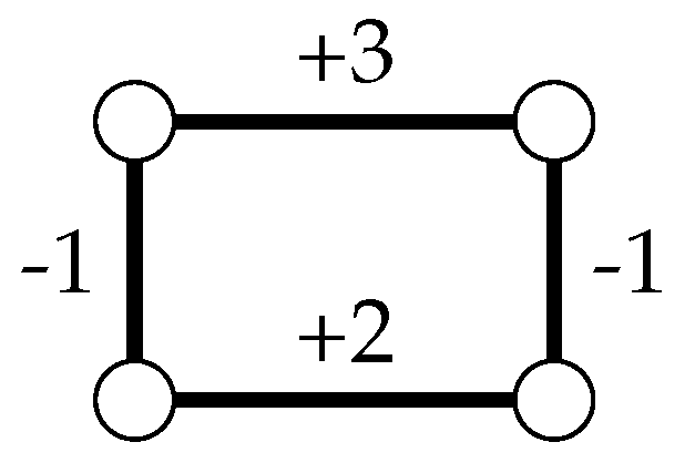
If the edges of G have signs, then one can define two different variants of clique-width for G. The unsigned clique-width of G is simply the clique-width of the graph obtained by removing all signs on the edges of G. On the other hand, the signed clique-width of G is the minimum k such that G can be defined by a signed k-expression, which is analogous to a k-expression with the sole distinction that the operation is replaced by which adds an edge with sign ℓ between all vertices labeled i and j. An example is provided in Figure 1.
We list a few known facts and observations about clique-width below:
- The difference between the signed clique-width (scw) and unsigned clique-width (cw) of a signed graph G can be arbitrarily large; more precisely, for every gap g there exists a signed graph G such that [25].
- Every signed graph of (signed) clique-width k can be defined by a (signed) k-expression which does not use the operator to create edges between vertices that are already adjacent (i.e., each edge is created only once).
- A signed k-expression of a bipartite signed graph G with bi-partition can be converted to a signed -expression of G such that the labels used for are completely disjoint from those used for (this is because any label that was originally used for and cannot be used to create new edges).
2.5. Graphical Representations
Here, we overview some natural graphical representations which have been used to capture the variable-constraint interactions of ILP instances. We remark that such representations are not unique to the ILP setting: indeed, they have been used and studied extensively also in settings such as, e.g., constraint programming [28,29] and Boolean satisfiability [11,30].
Let A be an integer matrix that is provided as part of an ILP instance . The signed incidence graph of A (or, equivalently, of ) is the edge-labeled bipartite graph , where contains one vertex for each row of A and contains one vertex for each column of A. There is an edge with label between the vertex and if , that is, if row r contains a nonzero coefficient in column c. In other words, the vertex set of is , a variable is adjacent to a constraint if and only if it occurs in that constraint with a non-zero coefficient, and the labels on edges encode this coefficient.
The incidence graph of A (or ), denoted , is equal to the signed incidence graph without the edge-labels. The primal graph of A (or ) is the graph , where C is the set of columns of A and whenever there exists a row of A with a nonzero coefficient in both columns c and . This graph is also sometimes called the Gaifman graph in the literature. The dual graph of A (or ) is the graph , where R is the set of rows of A and whenever there exists a column of A with a nonzero coefficient in both rows r and . In other words, the vertex sets of these graphs are and , respectively; an edge then signifies that two variables directly interact via a constraint or that two constraints directly interact via a variable, respectively. For all graph representations introduced above, we drop the in the parenthesis when the instance is clear from context. Figure 2 illustrates the four graphical representations of a constraint matrix.
For a decompositional width measure , we denote by , , , , the width of the signed incidence graph, the incidence graph, the primal graph, and the dual graph of , respectively.
2.6. Representation Stability
Changing between the equality and inequality representations for ILP does not have a significant effect on most of the structural parameters considered in this paper. In particular, it is easy to show that the parameters td, tw, cw, scw as well as the parameters fracture number (frac) and torso-width (defined in Section 5) differ at most by a factor of two when switching between the two representations. To see this it suffices to consider the standard transformations between ILP and ILP, which are given as follows.
Given an instance of ILP, we obtain an equivalent instance of ILP by replacing every equality constraint of with two inequality constraints and by adding the lower and upper bounds for the variables to the constraint matrix. It is easy to see that this transformation increases the above mentioned parameters for the primal, dual, and incidence graph by at most a factor of two.
Similarly, given an instance of ILP, we obtain an equivalent instance of ILP by introducing (i.e., adding) one novel “slack” variable to every constraint with a lower bound of 0. It is, similarly to the previous case, straightforward to show that this does not increase any of the considered parameters by more than a factor of two. As a consequence, for the statement of most of our complexity results we will simply consider instances of ILP and/or ILPF (which may be given in equality as well as in inequality form).
3. Solving ILPs with Explicit Restrictions
Initial work on mapping the complexity of integer linear programming predominantly focused on identifying tractable classes by placing restrictions on explicit properties of instances, such as the number of variables or of constraints. Lenstra [8] showed that ILP can be solved by an algorithm which has an exponential dependency on the number of variables, but only a linear dependency on the size of the instance. His running time was subsequently improved by Kannan [9] and Frank and Tardos [10].
Theorem 1
Papadimitriou showed that ILP is fixed-parameter tractable parameterized by [31]. His result was recently improved by Eisenbrand and Weismantel [32], and then further improved by Jansen and Rohwedder [33]. Even more recently, Knop, Pilipczuk and Wrochna showed that the running time of this result cannot be substantially improved [34].
Theorem 2
On the other hand, ILP remains intractable when all other obvious numerical measures are bounded. In particular, ILPF remains NP-complete even when and , as witnessed by the folklore encoding of the Vertex Cover problem into ILP, i.e., given a graph G and an integer k, the ILP instance has one binary variable for every vertex of G (representing of whether or not the vertex is chosen to be in a vertex cover) and for every edge between u and v a constraint ensuring that the sum of the variables for u and v is at least one (ensuring that the vertex cover contains at least one vertex from every edge).
While this is not the focus of this survey, we also mention that there is a significant body of work on exploiting algebraic properties to solve ILP. Perhaps the most prominent example of a complexity result obtained in this vein is the well-known fact that instances whose matrix A is totally unimodular (i.e., each of its square submatrices has a determinant in ) can be solved in polynomial time [35]).
Theorem 3
We say that an ILP instance is non-negative if all entries of A and b are non-negative. Cunningham and Geelen [37] showed that non-negative ILP is fixed-parameter tractable parameterized by and , where is the branchwidth of the column-matroid of A, i.e., the matroid whose elements are the column vectors of A and whose independent sets are the set of all linearly independent column vectors.
Theorem 4
([37]). A non-negative ILP instance with m constraints and n variables can be solved in time , where ω is equal to the branchwidth of the column-matroid of A.
4. Parameters for Sparse Variable-Constraint Interactions: Treewidth and Treedepth
We note that due to the discussion at the end of Section 2.5 all the results presented in this section hold regardless of whether our instance is provided in inequality or equality form. In 2015, Jansen and Kratsch [36] showed that the treewidth of the primal graph can be used to efficiently solve ILP when the variable domains are bounded by the parameter. More precisely:
Theorem 5
([36]). Let c be a constant. Given an ILPF instance with unary bounded domain satisfying the property that all but at most c variables have domain span at most d, and let be the primal graph of . Then admits a fixed-parameter algorithm when parameterized by .
The result follows from standard leaves-to-root dynamic programming along a tree decomposition of , and can be straightforwardly adapted to also solve ILP. This result provides a useful tool for dealing with instances where all variables have bounded domain. One year after Jansen and Kratsch’s result, Ganian and Ordyniak used a reduction from Subset Sum to rule out the application of treewidth In the setting of unbounded domain—even for extremely restricted instances of ILPF.
Theorem 6
In the same paper, Ganian and Ordyniak complemented this result with a fixed-parameter algorithm for ILP parameterized by ; the proof uses a pruning technique which transforms the instance into an equivalent one of size bounded by the parameter (a “kernel”). Their result was later superseded by Koutecký, Levin and Onn [39], who used Graver-best oracles to show:
Theorem 7
We note that both parameters and are required to achieve even XP algorithms: it is well known that ILP is NP-hard when restricted to instances with , and Ganian and Ordyniak [38] showed that it is also NP-hard when restricted to instances with . It is worth noting that both Theorem 7 and its predecessor have a non-elementary dependency on the parameter.
In their paper, Koutecký, Levin and Onn also used the same techniques to obtain a fixed-parameter algorithm that uses the treedepth of the dual graph (as opposed to the primal one):
Theorem 8
They also established an analogue to Theorem 6 for dual graphs, showing that restricting the dual or primal graphs leads to a similar complexity behavior for ILP:
Theorem 9
Since the classical encoding of Subset Sum into an instance of ILPF only uses a single constraint (i.e., ), it is immediate that ILPF is also NP-complete when ; in other words, it is not possible to strengthen Theorem 8 by dropping any of the parameters. By the standard reduction from Subset Sum we mean the reduction to the ILP instance that has one binary variable for every integer in the Subset Sum instance (representing whether or not the integer is in a solution) and one constraint over all variables ensuring that the sum of all chosen integers equals the target value of the Subset Sum instance.
The third fundamental graph representation that has been considered for restricting the variable-constraint interactions of an ILP instance is the incidence graph. It is worth noting that a trivial transformation of the respective decompositions yields and similarly ; on the other hand, there are instances where both and are bounded but the dual and primal graphs exhibit neither bounded treewidth nor treedepth. Hence, tractability results using the treewidth and treedepth of the incidence graph have the potential to supersede similar results for both previously considered graph representations, while any obtained hardness results carry over from primal and dual graphs to incidence graphs.
Ganian, Ordyniak and Ramanujan [40] identified conditions under which can be used to obtain algorithms for ILP. Notably, after factoring in Proposition 1 their result states:
Theorem 10.
ILPcan be solved in time , where Γ is the maximum absolute value of any partial evaluation of a constraint by any feasible assignment of ; here, a partial evaluation of a constraint/row of A with a feasible assignment is equal to , where is any vector obtained from after setting some of its entries to 0.
Note that , where d is the maximum domain span of every variable in . Hence, Theorem 10, e.g., implies that fully unary ILP can be solved in polynomial-time if is bounded by a constant.
On the other hand, ILPF remains NP-complete even when restricted to instances with strong restrictions on the treewidth and coefficients—to some extent justifying the dependency of the above algorithm on . Indeed, the first part of the following theorem follows from the classical encoding of Subset Sum into ILPF, while the second part was shown by Ganian et al. [40].
Theorem 11.
ILPFremainsNP-complete even on instances with (1) and Boolean domains for all variables, as well as with (2) and .
A natural question is whether one can use instead of in order to obtain tractability for ILP under a weaker restriction than by bounding —notably, can one lift Theorems 7 and 8 to the incidence treedepth setting? Very recently, Eiben et al. [41] answered the question in the negative by showing:
Theorem 12
In the full version of that paper, they also showed that restricting the structure by the size of a minimum vertex cover of —a significantly stronger restriction than treedepth—leads to tractability.
Theorem 13.
ILPisFPTparameterized by and the vertex cover number of .
Note that even though the vertex cover number is sensitive to changes between the equality and inequality form of ILP in general, the above theorem still holds for both forms. This is because the proof of Theorem 13 works by first observing that the number of (linearly independent) equalities is bounded by a function of the vertex cover number and and then uses Theorem 2 to show tractability. Almost the same approach can be used for inequalities, i.e., one can again observe that the number of inequalities is bounded in terms of the parameters (otherwise there are redundant inequalities) and then use the standard reduction from ILP to ILP; since the reduction does not increase the number of constraints, one can again apply Theorem 2.
We conclude this section by touching on the complexity of integer linear programs whose graph representations have an extremely simple structure—notably, have treewidth 1 (i.e., are acyclic). This setting was investigated by Eiben et al. [42], who showed that ILP restricted to unary instances whose graph representations are acycllic exhibit a different complexity behavior than ILP restricted to instances of bounded treewidth. We summarize their results in Table 1.
5. Other Parameters Exploiting Variable-Constraint Interactions
Of course, ILP has also been studied through the lens of structural parameters that are different than treewidth. The first example of such a parameter is the fracture number of Dvořák et al. [43], which captures the “distance” of an ILP instance from being fractured into small independent components.
Three variants of the fracture number will be of interest for the purposes of this survey: the constraint fracture number of an ILP () is the minimum number ℓ of constraints that need to be deleted from so that the resulting instance satisfies the following: each connected component of contains at most ℓ vertices. The variable fracture number () and mixed fracture number () are then defined analogously, with the distinction that we may only delete variables or are allowed to delete both variables and constraints, respectively.
The constraint fracture number is bounded whenever the dual graph has bounded treedepth, and the mixed fracture number is bounded whenever the incidence graph has bounded treedepth (and similarily for the variables fracture number and the primal graph); however, the converse of these statements is not true. Intuitively, this means that the fracture number can be viewed as a stronger restriction than treedepth. Dvořák et al. [43] showed that the fracture number can be used to obtain XP-algorithms for ILP in settings which would remain NP-hard if treedepth were used instead (see Theorem 12). See Figure 3 for an illustration of the relationships between the different variants of fracture number as well as their relation to treewidth and treedepth.
Theorem 14
Theorem 15
Note that theorem 15 cannot be improved to an FPT-algorithm due to (Theorem 14, [43]). Moreover, an analogous result does not hold for the mixed respectively variable fracture number as already unary ILP is NP-hard if the variable fracture number is bounded by a constant (Theorem 13, [43]), which also excludes the use of a less restrictive parameter than constraint fracture number (such as treedepth) in Theorem 15.
Another structural parameter that can be used to solve ILP is the torso-width. The base idea behind torso-width is to decompose instances into (possibly many) separate parts with only limited interaction between them, and to solve some parts with Lenstra’s algorithm (Theorem 1) and others with dynamic programming along a tree decomposition as per Theorem 5.
To define torso-width, we will need the operation of collapsing: for a graph G and a vertex set X, the operation of collapsing X deletes X from the graph and adds an edge between each pair of neighbors of X. We denote the resulting graph . Now, let q be a fixed constant. A graph G is a q-torso of iff there exists a set P of variables, each with domain span at most q, such that . The q-torso-width of , denoted , is then the minimum integer k such that has a q-torso G such that:
- G has treewidth at most k, and
- the largest connected component of the subgraph of induced on contains at most k vertices.
Ganian, Ordyniak and Ramanujan [40] showed that the q-torso-width of can be approximated by a fixed-parameter algorithm, and that this parameter can also be used to solve ILP. This result can be seen as a generalization of Theorem 1 as well as Theorem 5.
Theorem 16
Eiben, Ganian, Knop and Ordyniak [42] also investigated the complexity of ILP with respect to the parameter clique-width. They showed (and it is also not difficult to observe) that ILPF remains NP-complete even when restricted to extremely simple instances whose incidence, primal, and/or dual graphs have bounded clique-width. However, ILP becomes polynomially tractable when restricted to unary instances of bounded signed clique-width (of their signed incidence graph), under the assumption that a suitable k-expression is provided in the input.
Theorem 17.
There exists an algorithm which takes as input a unary instance ofILPand a signed k-expression tree T of , runs in time , and solves .
6. Summary and Future Work
This survey provides an overview of recently obtained (as well as previously known) (in-)tractability results for ILP with a focus on structural restrictions of the primal, dual, and incidence graph. The classes based on fracture number and treedepth can alternatively be defined in terms of block matrices and are also known as n-fold, tree-fold, 2-stage stochastic, and multi-stage stochastic integer linear programs; a recent and comprehensive overview for these classes, their exact relation to the classes considered in this survey, as well as the current best algorithmic approaches and techniques employed for these classes is given in [44].
Even though the complexity of ILP w.r.t. decompositional parameters such as treedepth, treewidth, and clique-width is by now quite well understood, we believe that the study of parameterized complexity of ILP is still in its infancy. Apart from studying more restrictive settings such as tree-like instances (in combination with, e.g., ) as well as related parameters such as feedback edge set, feedback vertex set, and bandwidth, we see at least two very promising directions for developing novel and even more general structural parameterizations: backdoor sets and hybrid parameters. Both of these approaches have already been successfully applied in settings such as Boolean Satisfiability and Constraint Satisfaction [29,45,46]. Informally, a backdoor set captures the situation when an instance is “close” to being tractable, and it looks promising to develop backdoor sets into one of the newly defined tractable classes. For instance, can we solve instances of ILP that differ from a known tractable class only by a small set of variables or constraints? Concerning the hybrid approach, where the aim is to solve instances consisting of many parts each of them tractable for a different reason, the number of possible directions seems even greater—torso-width is thus far the only explored hybrid parameter and many more tractable classes of ILP have been discovered since its introduction. Finally, it is important to explore if, how, and how far the known tractable fragments for ILP can be employed for well-known generalizations of ILP such as mixed or quadratic integer programs.
Author Contributions
Conceptualization, R.G. and S.O.; Writing—original draft, R.G. and S.O.
Funding
Robert Ganian acknowledges support from the Austrian Science Fund (FWF, Project P31336).
Acknowledgments
Open Access Funding by the Austrian Science Fund (FWF).
Conflicts of Interest
The authors declare no conflict of interest.
References
- Floudas, C.; Lin, X. Mixed Integer Linear Programming in Process Scheduling: Modeling, Algorithms, and Applications. Ann. Oper. Res. 2005, 139, 131–162. [Google Scholar] [CrossRef]
- van den Briel, M.; Vossen, T.; Kambhampati, S. Reviving Integer Programming Approaches for AI Planning: A Branch-and-Cut Framework. In Proceedings of the Fifteenth International Conference on Automated Planning and Scheduling (ICAPS 2005), Monterey, CA, USA, 5–10 June 2005; Biundo, S., Myers, K.L., Rajan, K., Eds.; AAAI: Menlo Park, CA, USA, 2005; pp. 310–319. [Google Scholar]
- Vossen, T.; Ball, M.O.; Lotem, A.; Nau, D.S. On the Use of Integer Programming Models in AI Planning. In Proceedings of the Sixteenth International Joint Conference on Artificial Intelligence (IJCAI 99), Stockholm, Sweden, 31 July–6 August 1999; Dean, T., Ed.; Morgan Kaufmann: San Francisco, CA, USA, 1999; Volume 2, pp. 304–309. [Google Scholar]
- Toth, P.; Vigo, D. (Eds.) The Vehicle Routing Problem; Society for Industrial and Applied Mathematics: Philadelphia, PA, USA, 2001. [Google Scholar]
- Lodi, A.; Martello, S.; Monaci, M. Two-dimensional packing problems: A survey. Eur. J. Oper. Res. 2002, 141, 241–252. [Google Scholar] [CrossRef]
- Alumur, S.A.; Kara, B.Y. Network hub location problems: The state of the art. Eur. J. Oper. Res. 2008, 190, 1–21. [Google Scholar] [CrossRef]
- Papadimitriou, C.H.; Steiglitz, K. Combinatorial Optimization: Algorithms and Complexity; Prentice-Hall: Upper Saddle River, NJ, USA, 1982. [Google Scholar]
- Lenstra, H.W., Jr. Integer programming with a fixed number of variables. Math. Oper. Res. 1983, 8, 538–548. [Google Scholar] [CrossRef]
- Kannan, R. Minkowski’s Convex Body Theorem and Integer Programming. Math. Oper. Res. 1987, 12, 415–440. [Google Scholar] [CrossRef]
- Frank, A.; Tardos, É. An application of simultaneous Diophantine approximation in combinatorial optimization. Combinatorica 1987, 7, 49–65. [Google Scholar] [CrossRef]
- Freuder, E.C. A Sufficient Condition for Backtrack-Bounded Search. J. ACM 1985, 32, 755–761. [Google Scholar] [CrossRef]
- Dechter, R.; Pearl, J. Tree Clustering for Constraint Networks. Artif. Intell. 1989, 38, 353–366. [Google Scholar] [CrossRef]
- Diestel, R. Graph Theory, 4th ed.; Graduate Texts in Mathematics; Springer: Berlin/Heidelberg, Germany, 2012; Volume 173. [Google Scholar]
- Cygan, M.; Fomin, F.V.; Kowalik, L.; Lokshtanov, D.; Marx, D.; Pilipczuk, M.; Pilipczuk, M.; Saurabh, S. Parameterized Algorithms; Springer: Berlin/Heidelberg, Germany, 2015. [Google Scholar]
- Flum, J.; Grohe, M. Parameterized Complexity Theory; Texts in Theoretical Computer Science. An EATCS Series; Springer: Berlin/Heidelberg, 2006; Volume XIV. [Google Scholar]
- Niedermeier, R. Invitation to Fixed-Parameter Algorithms; Oxford University Press: Oxford, UK, 2006. [Google Scholar]
- Downey, R.G.; Fellows, M.R. Fundamentals of Parameterized Complexity; Texts in Computer Science; Springer: London, UK, 2013; pp. 3–707. [Google Scholar]
- Kloks, T. Treewidth: Computations and Approximations; Springer: Berlin, Germany, 1994. [Google Scholar]
- Bodlaender, H.L. A linear-time algorithm for finding tree-decompositions of small treewidth. SIAM J. Comput. 1996, 25, 1305–1317. [Google Scholar] [CrossRef]
- Bodlaender, H.L.; Drange, P.G.; Dregi, M.S.; Fomin, F.V.; Lokshtanov, D.; Pilipczuk, M. A ck n 5-Approximation Algorithm for Treewidth. SIAM J. Comput. 2016, 45, 317–378. [Google Scholar] [CrossRef]
- Nešetřil, J.; Ossona de Mendez, P. Sparsity: Graphs, Structures, and Algorithms; Algorithms and Combinatorics; Springer: Berlin/Heidelberg, Germany, 2012; Volume 28. [Google Scholar]
- Courcelle, B.; Makowsky, J.A.; Rotics, U. Linear time solvable optimization problems on graphs of bounded clique-width. Theory Comput. Syst. 2000, 33, 125–150. [Google Scholar] [CrossRef]
- Courcelle, B.; Olariu, S. Upper bounds to the clique width of graphs. Discret. Appl. Math. 2000, 101, 77–114. [Google Scholar] [CrossRef]
- Golumbic, M.C.; Rotics, U. On the clique-width of some perfect graph classes. Int. J. Found. Comput. Sci. 2000, 11, 423–443. [Google Scholar] [CrossRef]
- Bliem, B.; Ordyniak, S.; Woltran, S. Clique-Width and Directed Width Measures for Answer-Set Programming. In Proceedings ECAI 2016—22nd European Conference on Artificial Intelligence; Kaminka, G.A., Fox, M., Bouquet, P., Hüllermeier, E., Dignum, V., Dignum, F., van Harmelen, F., Eds.; IOS Press: Amsterdam, The Netherlands, 2016; Volume 285, pp. 1105–1113. [Google Scholar]
- Oum, S.; Seymour, P.D. Approximating clique-width and branch-width. J. Comb. Theory Ser. B 2006, 96, 514–528. [Google Scholar] [CrossRef]
- Kanté, M.M.; Rao, M. The Rank-Width of Edge-Coloured Graphs. Theory Comput. Syst. 2013, 52, 599–644. [Google Scholar] [CrossRef]
- Samer, M.; Szeider, S. Constraint satisfaction with bounded treewidth revisited. J. Comput. Syst. Sci. 2010, 76, 103–114. [Google Scholar] [CrossRef]
- Ganian, R.; Ramanujan, M.S.; Szeider, S. Discovering Archipelagos of Tractability for Constraint Satisfaction and Counting. ACM Trans. Algorithms 2017, 13, 29:1–29:32. [Google Scholar] [CrossRef]
- Samer, M.; Szeider, S. Fixed-Parameter Tractability. In Handbook of Satisfiability; Biere, A., Heule, M., van Maaren, H., Walsh, T., Eds.; IOS Press: Amsterdam, The Netherlands, 2009; Chapter 13; pp. 425–454. [Google Scholar]
- Papadimitriou, C.H. On the Complexity of Integer Programming. J. ACM 1981, 28, 765–768. [Google Scholar] [CrossRef]
- Eisenbrand, F.; Weismantel, R. Proximity results and faster algorithms for Integer Programming using the Steinitz Lemma. In Proceedings of the Twenty-Ninth Annual ACM-SIAM Symposium on Discrete Algorithms (SODA 2018), New Orleans, LA, USA, 7–10 January 2018; pp. 808–816. [Google Scholar]
- Jansen, K.; Rohwedder, L. On integer programming and convolution. In Proceedings of the 10th Innovations in Theoretical Computer Science Conference (ITCS 2019), San Diego, CA, USA, 10–12 January 2019; pp. 43:1–43:17. [Google Scholar]
- Knop, D.; Pilipczuk, M.; Wrochna, M. Tight complexity lower bounds for integer linear programming with few constraints. In Proceedings of the 36th International Symposium on Theoretical Aspects of Computer Science (STACS 2019), Berlin, Germany, 13–16 March 2019; pp. 44:1–44:15. [Google Scholar]
- Schrijver, A. Combinatorial Optimization—Polyhedra and Efficiency; Springer: Berlin, Germany, 2003. [Google Scholar]
- Jansen, B.M.P.; Kratsch, S. A structural approach to kernels for ILPs: Treewidth and total unimodularity. In Proceedings of the Algorithms—ESA 2015—23rd Annual European Symposium, Patras, Greece, 14–16 September 2015; Bansal, N., Finocchi, I., Eds.; Lecture Notes in Computer Science. Springer: Cham, Switzerland, 2015; Volume 9294, pp. 779–791. [Google Scholar]
- Cunningham, W.H.; Geelen, J. On integer programming and the branch-width of the constraint matrix. In Proceedings of the 12th International IPCO Conference on Integer Programming and Combinatorial Optimization, Ithaca, NY, USA, 25–27 June 2007; Fischetti, M., Williamson, D.P., Eds.; Lecture Notes in Computer Science. Springer: Berlin/Heidelberg, Germany, 2007; Volume 4513, pp. 158–166. [Google Scholar]
- Ganian, R.; Ordyniak, S. The complexity landscape of decompositional parameters for ILP. Artif. Intell. 2018, 257, 61–71. [Google Scholar] [CrossRef] [Green Version]
- Koutecký, M.; Levin, A.; Onn, S. A parameterized strongly polynomial algorithm for block structured integer programs. In Proceedings of the 45th International Colloquium on Automata, Languages, and Programming, Prague, Czech Republic, 9–13 July 2018; pp. 85:1–85:14. [Google Scholar]
- Ganian, R.; Ordyniak, S.; Ramanujan, M.S. Going beyond primal treewidth for (M)ILP. In Proceedings of the Thirty-First AAAI Conference on Artificial Intelligence, San Francisco, CA, USA, 4–9 February 2017; Singh, S.P., Markovitch, S., Eds.; AAAI Press: Menlo Park, CA, USA, 2017; pp. 815–821. [Google Scholar]
- Eiben, E.; Ganian, R.; Knop, D.; Ordyniak, S.; Pilipczuk, M.; Wrochna, M. Integer Programming and Incidence Treedepth. In Proceedings of the Integer Programming and Combinatorial Optimization—20th International Conference (IPCO 2019), Ann Arbor, MI, USA, 22–24 May 2019; pp. 194–204. [Google Scholar]
- Eiben, E.; Ganian, R.; Knop, D.; Ordyniak, S. Unary Integer Linear Programming with Structural Restrictions. In Proceedings of the Twenty-Seventh International Joint Conference on Artificial Intelligence (IJCAI 2018), Stockholm, Sweden, 13–19 July 2018; pp. 1284–1290. [Google Scholar]
- Dvořák, P.; Eiben, E.; Ganian, R.; Knop, D.; Ordyniak, S. Solving Integer Linear Programs with a Small Number of Global Variables and Constraints. In Proceedings of the Twenty-Sixth International Joint Conference on Artificial Intelligence, Melbourne, Australia, 19–25 August 2017; Sierra, C., Ed.; IJCAI: Freiburg, Germany, 2017; pp. 607–613. [Google Scholar]
- Eisenbrand, F.; Hunkenschröder, C.; Klein, K.; Koutecký, M.; Levin, A.; Onn, S. An algorithmic theory of integer programming. Mathematics 2019, arXiv:1904.01361. [Google Scholar]
- Gaspers, S.; Szeider, S. Backdoors to satisfaction. In The Multivariate Algorithmic Revolution and Beyond—Essays Dedicated to Michael R. Fellows on the Occasion of His 60th Birthday; Bodlaender, H.L., Downey, R., Fomin, F.V., Marx, D., Eds.; Lecture Notes in Computer Science; Springer: Berlin/Heidelberg, Germany, 2012; Volume 7370, pp. 287–317. [Google Scholar]
- Gaspers, S.; Ordyniak, S.; Szeider, S. Backdoor Sets for CSP. In The Constraint Satisfaction Problem: Complexity and Approximability; Schloss Dagstuhl—Leibniz-Zentrum fuer Informatik: Dagstuhl, Germany, 2017; pp. 137–157. [Google Scholar]
Figure 1.
An example of a graph with clique-width 2 and signed clique-width 4.

Figure 2.
The primal, dual, incidence, and signed incidence graph of the constraint matrix shown in the top left corner. Vertices corresponding to variables (constraints) of the matrix are indicated by circles (rectangles). The label of a vertex corresponds to its row/column-index in the constraint matrix.

Figure 3.
The relationship between the structural parameters treewidth, treedepth, and fracture number for the primal, dual, and incidence graph. An arc from one parameter to another indicates that the former is a more general parameter, i.e., whenever the later is bounded so is the former. The variable, constraint, and mixed fracture number are defined in Section 5.


Table 1.
The complexity map for ILP for unary instances (first row), instances whose coefficients are encoded in unary (second row), and instances with unary bounded domain (third row). Without these restrictions, the problem becomes intractable due to the simple acyclic structure of the classical encoding of Subset Sum into ILP.
| Acyclic Primal Graph | Acyclic Incidence Graph | ||
|---|---|---|---|
| ILPF | ILP | ||
| Unary | P | P | P |
| Unary-C | NP-hard | P | NP-hard |
| Unary-D | P | P | NP-hard |
© 2019 by the authors. Licensee MDPI, Basel, Switzerland. This article is an open access article distributed under the terms and conditions of the Creative Commons Attribution (CC BY) license (http://creativecommons.org/licenses/by/4.0/).
Share and Cite
MDPI and ACS Style
Ganian, R.; Ordyniak, S. Solving Integer Linear Programs by Exploiting Variable-Constraint Interactions: A Survey. Algorithms 2019, 12, 248. https://0-doi-org.brum.beds.ac.uk/10.3390/a12120248
AMA Style
Ganian R, Ordyniak S. Solving Integer Linear Programs by Exploiting Variable-Constraint Interactions: A Survey. Algorithms. 2019; 12(12):248. https://0-doi-org.brum.beds.ac.uk/10.3390/a12120248
Chicago/Turabian StyleGanian, Robert, and Sebastian Ordyniak. 2019. "Solving Integer Linear Programs by Exploiting Variable-Constraint Interactions: A Survey" Algorithms 12, no. 12: 248. https://0-doi-org.brum.beds.ac.uk/10.3390/a12120248
Note that from the first issue of 2016, this journal uses article numbers instead of page numbers. See further details here.