Application of the Approximate Bayesian Computation Algorithm to Gamma-Ray Spectroscopy

1
Statistical Sciences, Los Alamos National Laboratory, Los Alamos, NM 87545, USA
2
Safeguards Science and Technology, Los Alamos National Laboratory, Los Alamos, NM 87545, USA
3
Advanced Nuclear Technology, Los Alamos National Laboratory, Los Alamos, NM 87545, USA
*
Author to whom correspondence should be addressed.
Algorithms 2020, 13(10), 265; https://0-doi-org.brum.beds.ac.uk/10.3390/a13100265
Submission received: 21 August 2020
/
Revised: 25 September 2020
/
Accepted: 14 October 2020
/
Published: 19 October 2020
(This article belongs to the Special Issue 2020 Selected Papers from Algorithms Editorial Board Members)
Abstract
:Radioisotope identification (RIID) algorithms for gamma-ray spectroscopy aim to infer what isotopes are present and in what amounts in test items. RIID algorithms either use all energy channels in the analysis region or only energy channels in and near identified peaks. Because many RIID algorithms rely on locating peaks and estimating each peak’s net area, peak location and peak area estimation algorithms continue to be developed for gamma-ray spectroscopy. This paper shows that approximate Bayesian computation (ABC) can be effective for peak location and area estimation. Algorithms to locate peaks can be applied to raw or smoothed data, and among several smoothing options, the iterative bias reduction algorithm (IBR) is recommended; the use of IBR with ABC is shown to potentially reduce uncertainty in peak location estimation. Extracted peak locations and areas can then be used as summary statistics in a new ABC-based RIID. ABC allows for easy experimentation with candidate summary statistics such as goodness-of-fit scores and peak areas that are extracted from relatively high dimensional gamma spectra with photopeaks (1024 or more energy channels) consisting of count rates versus energy for a large number of gamma energies.
1. Introduction
The energy spectra of gamma-rays emitted by radioisotopes act as fingerprints that enable the identification of the source. Such identification over short time periods is challenging for several reasons, including Poisson fluctuations in counts, relatively large isotope libraries with some peak overlaps, environmental effects, shielding effects such as missing peaks, single-escape and double-escape peaks due to electron pair production, pulse pileup and deadtime effects at relatively high count rates, as well as energy-dependent and sample-dependent detector efficiencies [1,2,3,4,5,6,7,8,9,10,11,12,13,14,15,16,17,18,19,20,21].
The term “unfolding” in gamma spectroscopy refers to several steps used to infer the features of the source that generated the spectrum [10]. The main gamma spectrum unfolding tasks are spectral data smoothing (as a form of noise reduction), background subtraction, peak searching (overlapping peak separation), peak area calculation, and radioisotope identification (RIID) [7,11].
There is reason to believe that RIID performance using, for example, Sodium Iodide (NaI) detectors (a very common fielded gamma ray detector) can be improved [7,8,9,10,11]. This paper will show the strong potential of approximate Bayesian computation (ABC) in peak location and area estimation, plus in simple RIID applications using either peak information or other features of the spectra collected by NaI detectors. Since [7], several RIID advances have been made. For example, [8] introduced a Bayesian approach applied to extracted peak locations and area ratios; [9] used convolution neural networks applied to simulated spectra; [10] applied the least absolute shrinkage and selection operator (LASSO) that is well known to be effective for subset selection. The first goal of an RIID algorithm is to choose which subset from a library of a few 10 s to approximately 100 radioisotopes (including medical, threat, industrial, and naturally occurring radioactive materials) is likely to be contained in a test item. The second goal is to estimate the amount of each isotope thought to be present in the item. One key validation step in any modern RIID is to simulate data assuming that the item contains the chosen isotope subset using a “forward model” that requires an estimate of the gamma detector response function (DRF) [11,12,13,18,19,20,21]. If the simulated data agree reasonably well with the observed data, then there is reasonable confidence that the inferred subset is at least close to correct. However, simulation model bias is not yet considered in any existing RIID to our knowledge. The ABC algorithm [22] provides a natural option to allow for model bias and this leads to the proposed new ABC-based RIID.
This paper is organized as follows. Section 2 provides additional background for gamma-ray spectroscopy. Section 3 briefly describes existing peak location algorithms. Section 4 briefly describes smoothing algorithms. Section 5 describes ABC and peak location and area estimation. Section 6 illustrates a newly developed ABC-based RIID.
2. Background
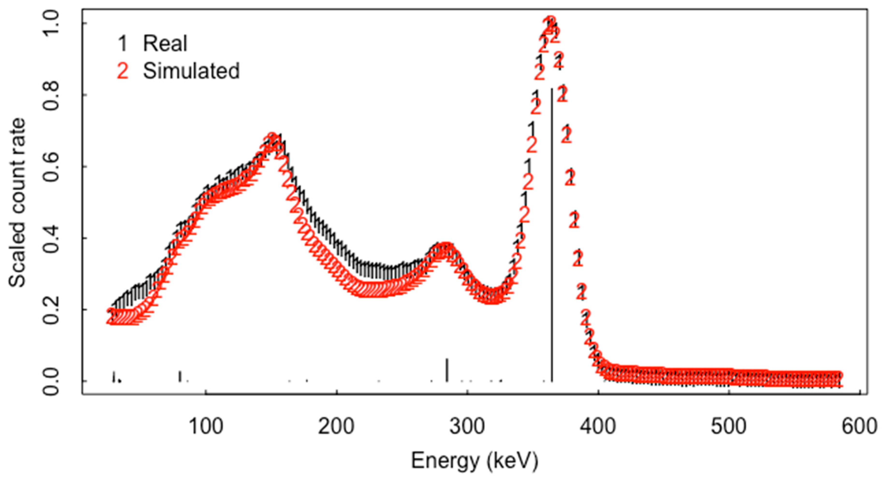
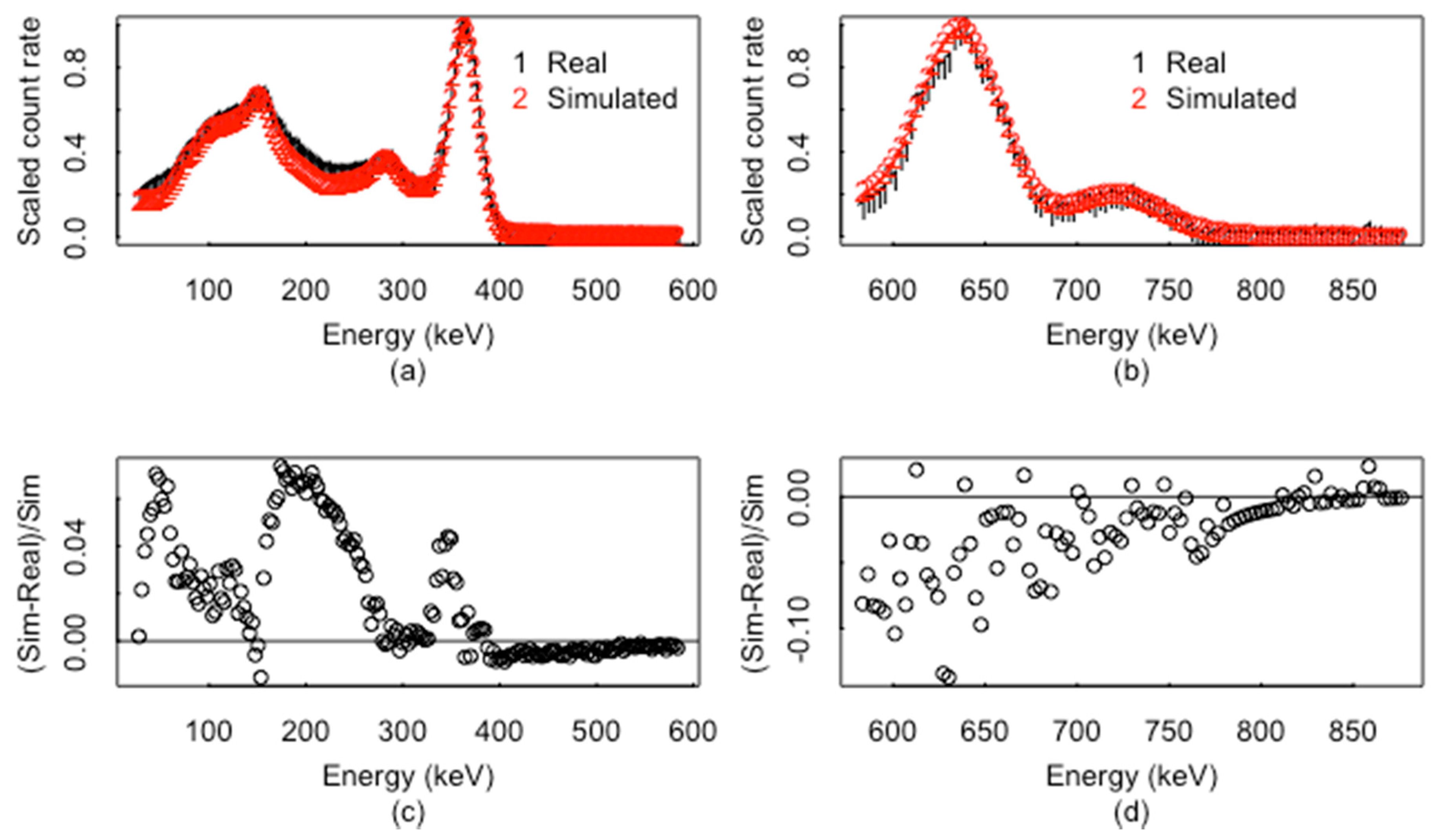
Figure 1 plots real (smoothed using the iterative bias reduction method [23,24]) and simulated spectra (from the GADRAS 18.8.10 code [21]) from a relatively low-energy resolution and widely deployed NaI detector of the isotope I-131 without shielding effects and with background effects subtracted. I-131 is a medical-use isotope that is sometimes detected at border crossings, is a radionuclide that vendor’s field instruments are required to recognize and is a significant fission product that can be released into the atmosphere. Shielding attenuates lower energy counts more than higher energy counts, and can reduce or sometimes eliminate evidence of low energy peaks. The vertical lines indicate the birth energies of the key source of gamma energies from the decay of I-131; note that some peaks are not likely to be detected. The approach and an example function to simulate such spectra are given later in the section. Figure 2 plots real and simulated spectra of I-131 for two energy ranges in Figure 2a,b, and the corresponding relative model bias calculated as (simulated/-measured)/simulated in Figure 2c,d. Other radioisotopes have different gamma birth energies with different relative intensities so in theory, the potential signature of most radioisotopes is at least moderately distinct from that of other isotopes. In practice, for relatively low resolution detector types such as NaI detectors (commonly deployed detector and the main type of interest here, although higher resolution is also discussed), RIID performance can be surprisingly poor [1,2,3,4,5,7,8,9,10,15,16,17].
Since the 2009 paper [7] on RIID algorithms, to infer what radioisotopes are present in an unknown test item, there have been several improvements to RIIDs for NaI spectra. Most notably, among those algorithms that rely on estimated peak locations and net areas, [8] developed a Bayesian approach, and [10] applied the LASSO. However, reference [8] did not address to what extent its Bayesian approach actually led to well calibrated probabilities that a given radioisotope was present in each test item. That is, among all test items for which the estimated posterior probability that isotope A was present is for example, approximately 90%, was the actual fraction that included A close to 90% [25,26,27]?
The ABC-based RIID reported in this paper is shown to be well calibrated, and it can rely (depending on the user choice of summary statistics) on locating peaks and estimating peak areas. Section 5 demonstrates that (1) the extracted peak areas are impacted by modeling bias and (2) that there can be some advantage in using non-parametric methods to estimate peak areas. Both parametric and nonparametric options are evaluated in real and simulated data. The parametric method must first select an analytical model such as the one used in the Gamma Detector Response and Analysis software (GADRAS [21]) or the one used in the Fixed Energy Response Function Analysis with Multiple Efficiencies software (FRAM [28]) and then estimate the model parameters. The DRF is a mapping from the gamma birth energy to the distribution of possible detected energies. The DRF must account for the main interactions of gamma rays in the detector, including photoelectric absorption, Compton scattering, and pair production, as well as the processes in the conversion process from deposited energy in the detector to a measured voltage pulse that leads to increased variance in the measured energy. Figure 1 is an illustration with the vertical lines depicting the gamma birth energies with the observed count rates in each energy bin arising from the probability of detecting a gamma with birth energy E1 at another energy E2. An example DRF (for a range of detector resolutions) is:
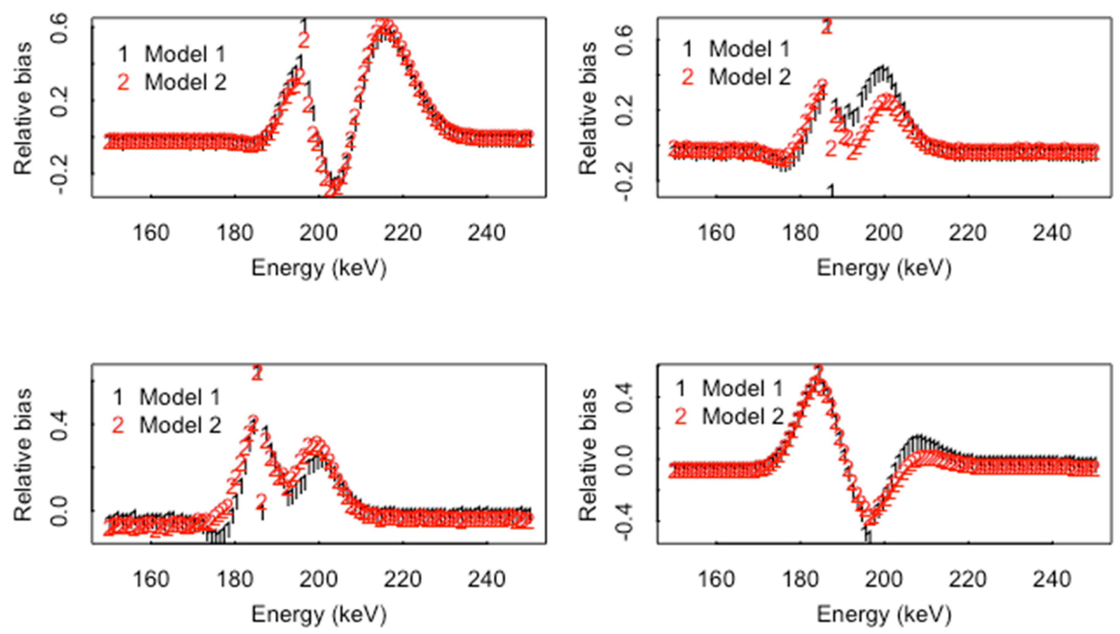
which defines a simplified version of a DRF in FRAM with the Gaussian broadening of each peak, plus a tail and background contribution from each peak (FRAM sets and sets . Previous versions of FRAM set = = 0 to get what is referred to as model 2 in Section 5. Model 1 allows for nonzero and and is currently thought to provide a better description of spectral data at least for higher resolution detectors with a large number of peaks and relatively large mean count rates. This example FRAM model is intended as a good approximation in a region close to a peak. Because the FRAM model does not account for scattering to lower energies outside of a small tail contribution, it is not a comprehensive DRF, and this explains why in Figure 2 the simulated spectrum drops more below the real spectrum more at lower energies away from the peak. The statistical programming language R [29] is used throughout this paper for analysis, and the DRF f(E) in Equation (1) is coded as an R function.
3. Peak Location Algorithms
One common peak location algorithm uses differences and second differences to locate each local maximum [30]. The first derivative changes sign from positive to zero to negative at a peak; therefore, the second derivative for automatic full-energy peak location was proposed by [30]. However, real spectra have significant fluctuations because of the discrete and statistical nature of the data. Thus, a discrete analog of the second derivative (the second difference) is typically used.
Each local maximum is a candidate peak, and simple screening methods can eliminate some local maxima from consideration. Two common screening methods are to check whether the local maximum is sufficiently larger than the nearby background level, which is larger than an absolute threshold, or the peak width is larger than a threshold.
No matter what peak detection and location methods are used, as seen in Figure 1, it is unlikely that all birth energies will lead to a detected peak. Whenever a peak detection algorithm fails to resolve overlapping peaks, some information will still be extracted from the resulting combined peaks. Therefore, library comparison RIIDs [1,2,3,4,5,6,7,8,9,10] have the potential to work better with customized libraries with a single peak energy and peak area assigned to a composite peak. For example, the libraries in [31] only save information regarding the combined peak. It is still necessary to assess whether a peak detection algorithm can resolve overlapping peaks. The minimum energy gap (minimum resolvable energy, MRE) that a peak detection algorithm can resolve can be estimated using real and/or simulated spectra. The MRE will be different for different peak detection algorithms and detector response functions, which depends on the relative amplitude of the adjacent peaks [8]. The Bayesian RIID in [8] used the photopeak libraries in [31] generated by the method in [8]; almost certainly the simulated spectra would be meaningfully different from corresponding real spectra; the impacts of simulation quality on RIID development and assessment will be addressed in future work.
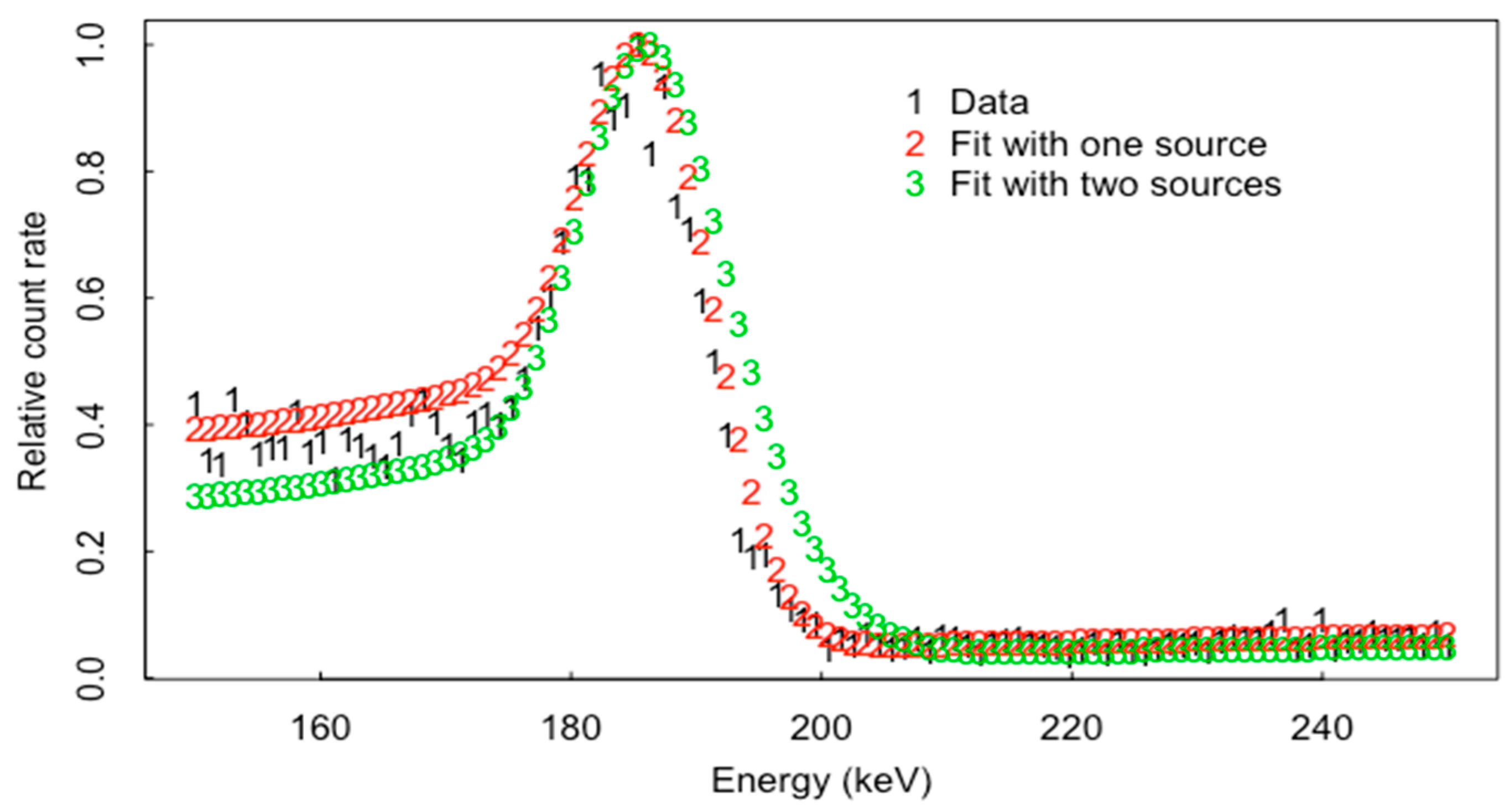
As an example, Figure 3 plots example raw data and a fit to one peak and a fit to two peaks. The fit with one peak leads to a different estimated peak center (centroid) and net peak area than does the fit with two peaks.
4. Smoothing Algorithms
Algorithms to locate peaks can be applied to raw or smoothed data, and among the smoothing options considered (including wavelet-based [32], spline-based, local-linear smoothing) the iterative bias reduction (IBR) algorithm has been shown to be effective [23,24] so it will be used here. The basis for assessing IBR effectiveness is the extensive testing results reported in [23] in which separate root mean squared error (RMSE) results were reported for on-peak and off-peak smoothing. The IBR algorithm is quite successful in adaptively smoothing to reduce bias in peak regions by smoothing less, and smooth more heavily in off-peak regions without explicitly identifying the peak regions.
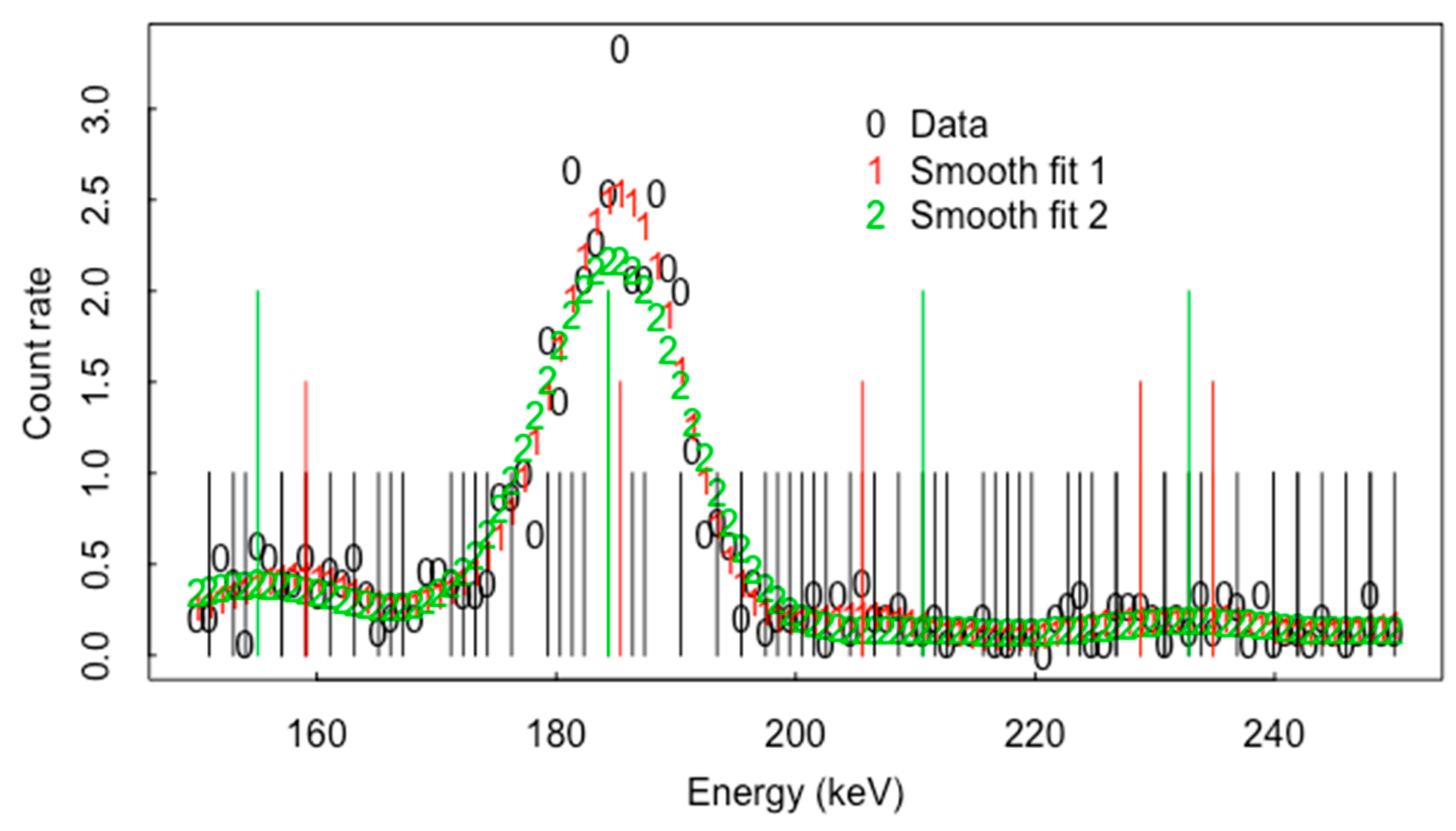
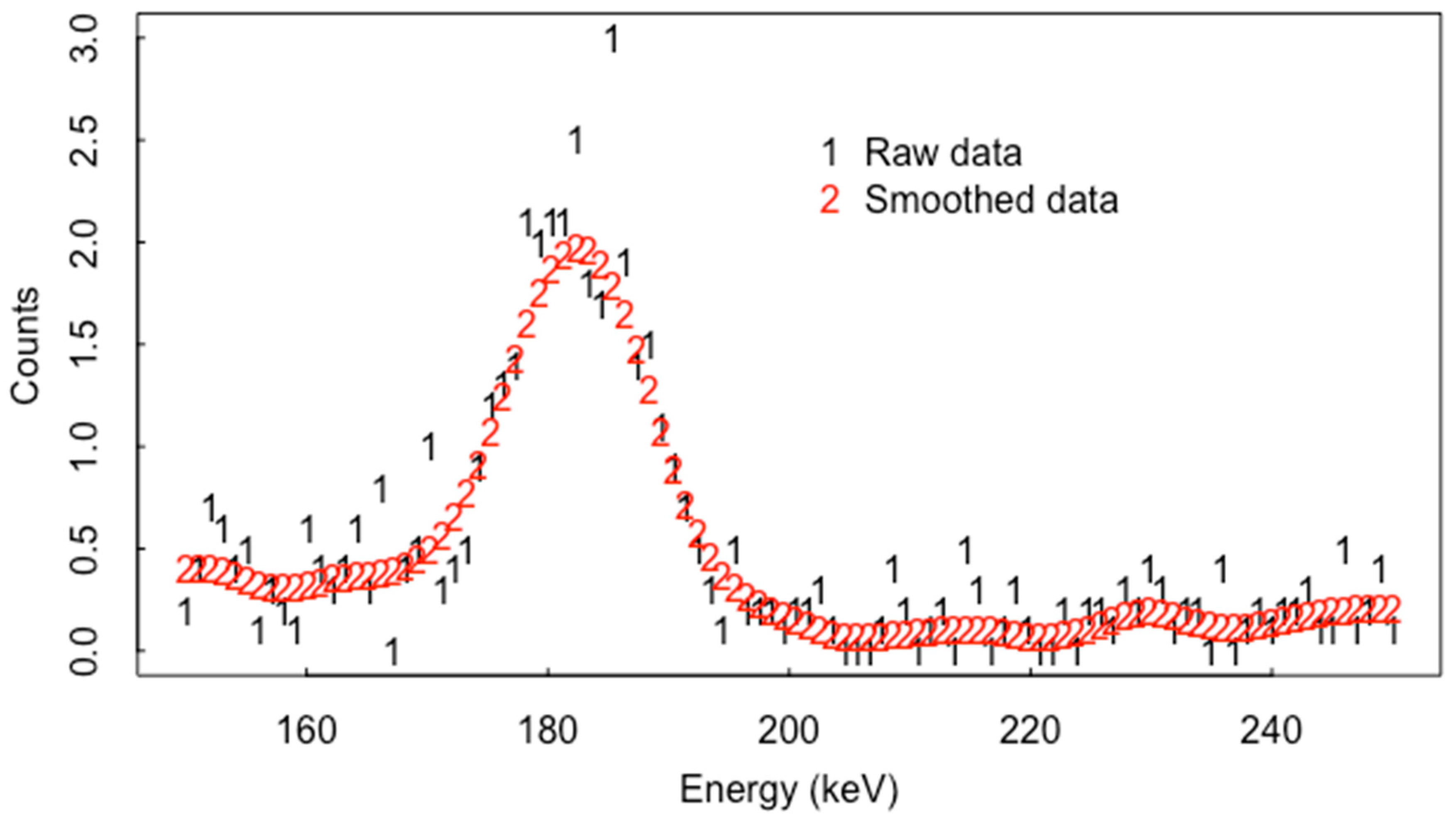
Smoothing data over neighboring energy bins can reduce noise in the raw counts, at the cost of introducing a bias that de-emphasizes the peaks and valleys of a spectrum. Reference [23] described a new two-stage smoothing procedure that uses a multiplicative bias correction (working with the ratio data/smooth) for adjusting initial smoothed spectra. Applying the multiplicative bias correction to an initial smoother reduces the bias of the initial smoother in the peaks and valleys with no or a negligible increase in its variance. As an example, Figure 4 is the real data (from an item enriched in U-235, for which the major peak is located at 185.7 keV) and two smooth fits using IBR. Smooth fit 2 uses fewer degrees of freedom (df) than smooth fit 1 and so smooth fit 2 oversmooths in the peak. In practice, the df is chosen using cross validation. The vertical black (red, green) lines are the local maxima in the raw data and smooth fit 1 and fit 2, respectively. The obvious peak near 185.7 is found using all three (raw, smooth 1 and smooth 2).
All smoothers exhibit bias to varying degrees in regions of rapid change such as near a peak. An ideal smoother smooths peak regions very little and off-peak regions much more [23]. The IBR algorithm evaluates the ratio data/smooth to detect regions of oversmoothing using iteration.
5. Net Peak Area Extraction and ABC
The net area of a peak can be estimated using a parametric or non-parametric approach. A parametric approach assumes an analytical function such as the f(E) in Equation (1). A nonparametric approach infers which energy bins belong to the peak region and uses a nearby background to estimate the background contribution to the gross peak count rate.
Recall that some RIIDs use estimated peak location and area. For example, reference [7] described the potential for a Bayesian RIID and reference [8] implemented one version of a Bayesian RIID that relied on peak locations and areas. Reference [8] assumed that the likelihood could be expressed as a product of four terms:
The term quantifies how well model matches expected library peaks, weighted by peak areas. Specifically, , where = 1 if the ith library peak (of L library peaks) is found in the data, is the estimated area of peak I and is a parameter to control the magnitude of the penalty for library peaks that are not found in the data. For example, if model M is isotope 1 without any other radioisotopes and isotope 1 has K = 3 library peaks, all of which are found in the data, then . Similarly, scores how well the D data peaks are matched in the L library peaks. The peak position score quantifies how closely the found peak is to the library peak, if and if . Allowing a nonzero value of was shown in [8] to perform better because it ensures that matched peaks lead to a larger likelihood than unmatched peaks. The area ratio quantifies how well the ratios of the data peak areas match the corresponding library peak ratios. Comparing area ratios rather than areas eliminates the need to estimate shielding (lower energy gammas are attenuated more than higher energy gammas by shielding, but by amounts that depend on the unknown types and amount of shielding) and to have a prior estimate of relative source activity. To define , a lower bound and upper bound are defined such that if the relative peak area for a matched peak lies between and . For larger discrepancy in the matched peak areas, an exponential decay in the penalty is used that allows for more widely separated matched peaks to differ more in area due to energy-dependent attenuation effects.
Reference [8] used a custom library that was created using simulated spectra from each isotope in the library [31]. This labor-intensive approach used the estimated minimum resolvable energy to create composite peaks, eliminating unresolvable peaks. To illustrate, several library peaks of I-131 do not appear to the eye of the measured I-131 spectrum in Figure 1 and would be unlikely to appear in the custom library in [31].
Although [8] reported stable posterior probability results for the two isotopes evaluated (Eu152 and Co60), clearly is ad hoc, and is not to be interpreted as a true likelihood. Therefore, there has been no attempt to quantify uncertainty in the model choice stage so [8] did not address to what extent its Bayesian approach actually led to well calibrated probabilities that a given isotope was present in each test item. That is, among all the test items for which the estimated posterior probability that isotope A was present was, for example, approximately 90%, was the actual fraction that included A close to 90%? Note that having well calibrated probabilities is desired, but the top priority is the highest correct classification rate; however, if a confidence measure such as the probability that the chosen model is correct is not well calibrated, then it will not provide value to the procedure.
5.1. ABC
Any Bayesian approach requires a prior probability and a likelihood to compute the posterior probability of model as , where is the likelihood and is the prior probability of model . The likelihood is key to any statistical approach, Bayesian or non-Bayesian (“frequentist”) [33,34].
ABC provides a way to modify the approach in [8] using summary statistics computed from spectra. The factors become candidate statistics for use by ABC. Other candidate statistics include one or multiple peak fits to key regions, off-peak count rates at selected energy bins, scan statistic values associated with chosen peaks, and the net signal attributable to each isotope in the library. The net signal for 1, 2, …, p peaks is the net signal-to-noise ratio assigned to the recognized peaks, where is the peak height (“signal”) for peak i and is the peak width for peak i. Recall that DRFs typically assume a Gaussian-shaped peak with a tail and background as f(E) in Equation (1). Because the number of candidate statistics is large, one could perform ABC separately for each library isotope, following the approach in [9,10].
In any Bayesian approach, prior information regarding the magnitudes and/or relative magnitudes of any model parameter(s) can be provided. If the prior is “conjugate” for the likelihood (for example, a gamma prior is conjugate for the Poisson likelihood), then the posterior is in the same likelihood family as the prior, in which case analytical methods are available to compute posterior prediction intervals for quantities of interest. So that a wide variety of priors and likelihoods can be accommodated, modern Bayesian methods do not rely on conjugate priors, but use numerical methods to obtain samples from approximate posterior distributions [34]. For numerical methods such as Markov Chain Monte Carlo [34], the user specifies a prior distribution (which need not be normal), for the parameters to be inferred, such as which subset of the library isotopes is present and in what amounts in the test item and possibly which shielding materials are present [3,5,30]. The user must also specify a likelihood for the data given the model parameters. In contrast, ABC does not require likelihood for the data; and, as in any Bayesian approach, ABC accommodates constraints on variances through prior distributions [22,25,26,33].
No matter what type of Bayesian approach is used, a well calibrated Bayesian approach is defined here as an approach that satisfies several requirements. One requirement is that in repeated applications of ABC, approximately 95% of the middle 95% of the posterior distribution for peak area (for example) should contain the true value. That is, the actual coverage should be closely approximated by the nominal coverage. The nominal coverage is obtained by using the quantiles of the estimated posterior. For example, the 0.005 and 0.995 quantiles define the lower and upper limits of a 99% probability interval. A second requirement is that the true mean squared error (MSE) of the ABC-based estimate of the peak area should be closely approximated by the variance of the ABC-based posterior distribution of peak area. Inference using ABC can be summarized as follows:
ABC Inference
For i in 1, 2, …, N (typically, N is large, such as 104 or 105 or more) do these three steps:
- (1)
- Sample from the prior, ;
- (2)
- Simulate data from the conditional pdf ;
- (3)
- Denote the real data as If the distance then accept as an observation from ;
Experience with ABC suggests that the ABC approximation to improves if step (3) is modified to include a weighting factor, so that trial values of simulated from that lead to very small distance are more heavily weighted in the estimated posterior [22,35]. In step (2), the model can be analytical or, for example, a forward transport model. In ABC, the model has input parameters θ, has output data , and there is corresponding real data xobs. For example, f(x) in Equation (1) is a forward model (with energy E denoted generically as x here) with 12 parameters (three for the peak: peak width, location, height; five for the tail associated with the dominant peak; and four for the background as modeled by P1–P4). Model parameter specifies which isotopes are present and in what amounts, and is the forward model such as Equation (1) or GADRAS [21].
To illustrate, 105 simulations of one-peak and two-peak regions (overlapping peaks) were simulated. Using ABC, when the true model was the same as the assumed model, parametric-based area estimation has a smaller RMSE than non-parametric estimation. However, when the assumed model is only modestly different from the true model, the non-parametric based area estimation has a lower RMSE (see below for more detail).
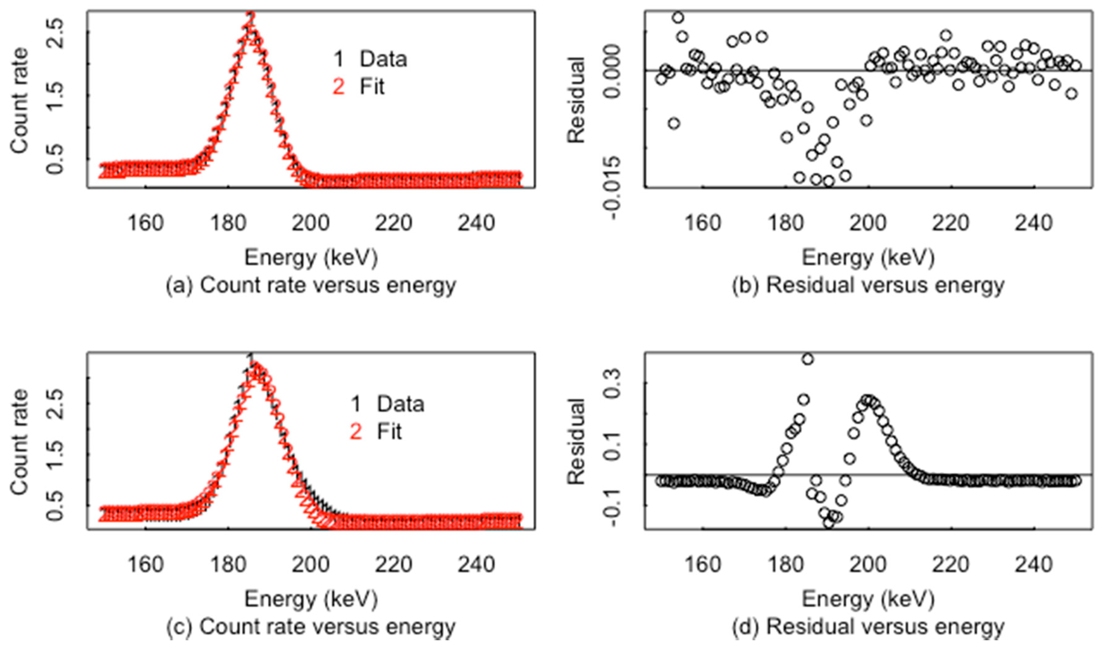
ABC is also effective for choosing the number of peaks in a region. For example, in a small energy region, either one or two peaks appear to be present to the eye. ABC sometimes chooses one peak, and sometimes chooses two peaks in simulated repeats of the same data. For example, Figure 5 plots the data and fit and the corresponding residuals defined as usual as residual = data − fit when the true data have one peak or two peaks and the fitted model always has one peak. The pattern and magnitude in the residuals in the peak region in both (b) and (d) suggests a much worse fit in (d). The residuals in (d) would be flagged by a scan statistic [35], leading to a rejection of the one-peak fit. A scan statistic scans for the largest sum of consecutive positive residuals; a separate scan statistic can be computed that scans for the smallest sum of consecutive negative residuals. Moreover, the maximum of the scan statistic over the analysis region can easily be included as a candidate summary statistic in ABC.
One nice feature of ABC is that the goodness-of-fit scores to compare fits with one, two, or more peaks can be used as summary statistics, which are used to approximate the posterior probability of a candidate set of model parameter values such as the isotopic composition of the item being assayed.
In any peak-fitting approach, one must choose the energy region using some type of figure of merit [36]. ABC also provides an option to choose the energy region for the analysis of residuals, using trial and error to determine which energy region leads to the best inference. To illustrate ABC, 100 energy bins were chosen that only included the dominant peak at 185.7 keV (from U-235); summary statistics included the maximum of each of two scan statistics (one scanning for a large sum of consecutive positive residuals between data and fit and the other scanning for a large sum of consecutive negative residuals), the average residual, and the minimum and maximum residual for a total of five candidate summary statistics scan statistics. In 105 test items and using a training size of 105 simulated data sets (using f(E) in Equation (1) with Poisson variation), the misclassification rate was 0.2% (134 misclassified out of 105, with 107 having two peaks classified as having one peak and 117 having one peak classified as having two peaks). Each simulated data set had one peak only with a probability of 0.5 and had the same peak plus a nearby peak at 187.7 keV with a probability of 0.5. All simulated data sets were normalized by dividing by the maximum count rate, so all scaled count values ranged from 0 to 1, to deliberately avoid trivially obvious discrimination (that would not be available in applications of interest) between the two classes (class 1 has one peak; class 2 has two peaks) based on the average count rate near the peak. ABC is thus showing strong potential for this type of model selection and will be further investigated for its potential in selecting the number of peaks present in an analysis region.
To illustrate, the peak location (center) and height were estimated using either parametric (using Equation (1)) or nonparametric estimation in ABC. One set of ABC runs used the parametric estimation results as summary statistics and a second set of ABC runs used the nonparametric estimation results as summary statistics. Simulation results indicate that ABC is well calibrated at the 90%, 95%, and 99% posterior probability intervals for each model parameter of ineptest, and provides an effective estimate of the RMSE in a frequentist sense, with the average posterior standard deviation across the 105 simulations in close agreement with the RMSE. Additionally, the RMSE in peak area estimation (peak area is calculated as from Equation (1)) is 0.28 (repeatable across sets of 105 simulations to within for the parametric based on simdata1 and 0.29 for the nonparametric method with the true model is the same as the assumed model (model 1 is the true model and model 1 is the assumed model with model 1 defined as in Figure 6). When the true model is model 1 but the assumed model is model 2 (by setting P2 = P4 = 0 in Equation (1) as explained in Section 2), the RMSE remains 0.29 for the nonparametric method but increases to 0.38 for the parametric method.
Recall that ABC does not require one to explicitly specify a likelihood. Therefore, the true likelihood used to generate the data need not be known to the user. Synthetic data are generated from the model for many trial values of and trial θ values are accepted as contributing to the estimated posterior distribution for θ|xobs if the distance , between , and is reasonably small. Alternatively, for most applications, it is necessary to reduce the dimension of xobs to a small set of summary statistics S and accept trial values of θ if , where is a user-chosen threshold. Here, for example, is the gamma count rate in a specified subset of energy channels, and specifies which isotopes are present and in what amounts.
Recall that, because trial values of θ are accepted if , an approximation error to the posterior distribution arises that several ABC options attempt to mitigate. Additionally, recall that such options weigh the accepted θ values by the actual distance (abctools package in R [33]). In practice, the true posterior distribution is not known, so a method such as that in [25,26,37] using the calibration checks described above, is needed in order to choose an effective value for the threshold.
ABC can be used to evaluate candidate summary statistics. For any inference option, the estimated distribution of plausible peak parameters (or isotope subset in the full RIID application) can be assessed by checking at least two criteria: (1) whether the estimated standard deviations agree with the observed standard deviations, and (2) whether the actual coverage of coverage intervals is close to the nominal. For example, a 95% probability interval construction method (frequentist or Bayesian) should contain the true nuclear material mass in approximately 95% of the repeated applications. ABC is used here for two main reasons:
- (A)
- ABC allows for an easy comparison of the performance of candidate summary statistics such as peak area ratios, off-peak count rates, and goodness-of-fit test results such as scan statistic values near peaks.
- (B)
- ABC allows for easy experimentation with different DRFs.
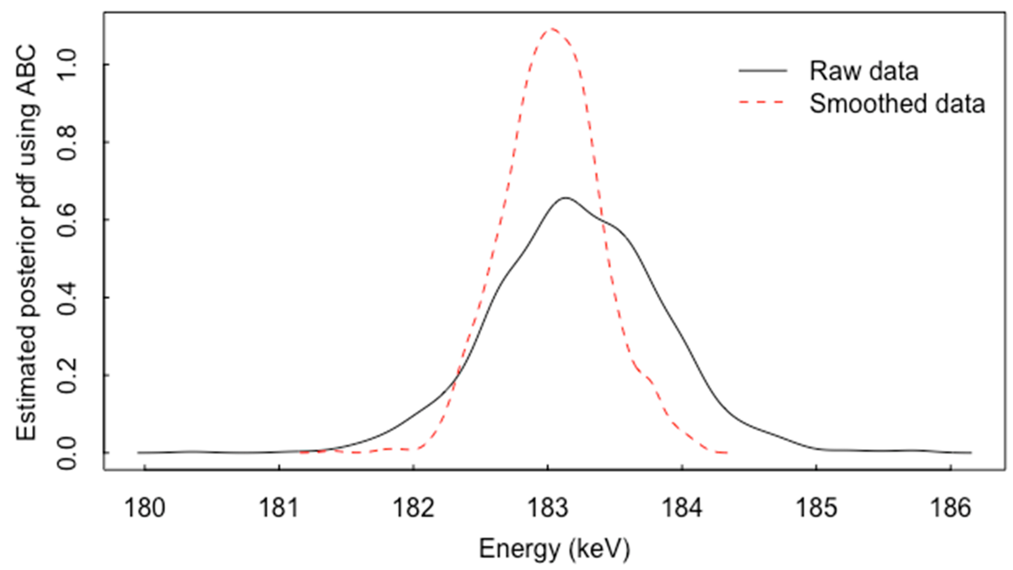
As an example, for the spectra in Figure 7, Figure 8 plots an ABC-based estimate of the posterior probability density function (pdf) for peak location, using either raw or smoothed data. To implement ABC, 105 simulations of both raw and smoothed spectra were generated by sampling from the prior distribution, which spanned a range of peak locations, areas, and widths. Note that the posterior is wider for the raw data; in this case, a short count time was simulated, resulting in 7000 counts over the 250 keV-wide region of interest, so smoothing has a large impact. In a separate set of 103 simulated test cases (the spectra in Figure 7 are test case number 1 of 1000), the ratio of the posterior standard deviation of the peak location distribution for smoothed spectra to that for raw spectra for peak location is approximately 0.45 (0.43/0.93 = 0.46), so the fact that the smoothed data lead to a narrower posterior for test case 1 is typical. For test case 1, the ratio of the standard deviation for the smoothed data to that for the raw data is 0.37/0.62 = 0.60. For area estimation, the ratio of the RMSE for the smoothed to that for the raw data is 1.41/1.84 = 0.77. Recall that the area is calculated as from Equation (1).
This observed tendency for the smoothed data to lead to a narrower posterior than the raw data do for peak location calls for attention to the “is ABC calibrated” question. Fortunately, ABC is shown here to again be well calibrated, with actual coverages of 0.89, 0.95, and 0.99, using the quantiles of the posterior to calculate the probability intervals having nominal coverages of 0.90, 0.95, and 0.99, respectively. Moreover, the average posterior standard deviation is {0.90 for the raw, 0.43 for the smoothed} while the observed RMSE is {0.90 for the raw data and 0.42 for the smoothed data}, indicating excellent agreement with both the coverage and the RMSE calibration checks. Therefore, smoothing appears to improve peak location estimation, at least when the raw data arises from moderate or short count times leading to a modest number of total counts (as is typical in applications).
6. A New ABC-Based RIID
During ABC-based RIID development, one can easily experiment with different summary statistics. Here, a very simple RIID was developed and applied as follows; future work will include factors such as from [8] described above as candidate summary statistics. In the simple RIID, smoothed data (using IBR) was used to locate peaks. Then, only those candidate peaks that were statistically distinct from the nearby background were used. Each significant peak’s area was estimated using the nonparametric peak area approach described in Section 4. The goal was to distinguish between four groups. Group 1 is simulated Lu-177m (“m” denotes a meta-stable isotope) spectra. Group 2 is the corresponding simulated Lu-177m spectra with model bias. Group 3 is the simulated weapons grade WgPu spectra; group 4 is the corresponding simulated WgPu spectra with model bias. The simulated Lu-177m and WgPu spectra are plotted in Figure 9.
Results of this very simple RIID are illustrated in Figure 10 and Figure 11. This is a simple RIID example because the library consists of only four groups and because the shape of the Lu177m spectra is not that difficult to distinguish from that of WgPu (although Lu177m was chosen because its spectrum is has certain similar features to that of WgPu that can cause some algorithms to misidentify it). In this ABC-based RIID example, simulated Lu-177m and simulated WgPu are to be distinguished. The simulations were done in GADRAS 18.8.10 [21], and simulation bias was estimated by comparing real to simulated spectra as in Figure 6. Four classes are in the training data for ABC. Summary statistics from the scaled count data in Figure 9, and from the scaled count data in Figure 9 that is modified by adding an estimated model bias vector to the Lu177m spectra, and a second estimated model bias vector to the WgPu spectra.
Figure 10 is a principle coordinate (PC) plot using the cmdscale function in [29]. The two plotted PCs can be used to closely approximate the distance between each of the 100 spectra (25 sets from each of the four groups) and give strong qualitative evidence that Lu177m spectra are distinct from the WgPu spectra. Figure 11 plots the results of a simple ABC-based RIID that aims to predict which group a test items is in (group 1 is Lu177m; group 2 is WgPu; group 3 is simulated Lu-177m with model bias; group 4 is simulated WgPu with model bias). As in Figure 1 for I-131, model bias is evident when any of the real spectra are compared to the corresponding simulated data. Therefore, model bias was simulated as follows. First, model bias was estimated for 10 real (background subtracted) and corresponding GADRAS-simulated isotopes as with the I-131 example in Figure 1. Second, principal components (the prcomp function in [29]) of the collection of bias vectors were calculated and the dominant five components were retained in order to capture most of the variability observed among the 10 estimated bias vectors. Third, to generate other model bias vectors B, small random variations (zero mean, 0.05 standard deviation random normal variables) were added to the mean coefficient vector to generate additional bias vectors . This is an ad hoc but defensible option to generate bias vectors on the basis of 10 paired comparisons between the real and simulated data. In Figure 10, the modeled bias vector was group-specific, so the five sets of values were only generated one time for the Lu177m isotope group and one time for the WgPu group.
For the same example, for one test case, Figure 11 plots the ABC-based probability for model 1, model 2, model 3, and model 4, with the true model being model 1 (a), model 2 (b), model 3 (c), or model 4 (d).
One calibration check in this ABC-based RIID is whether the estimated posterior probability of the chosen model provides a good measure of confidence. Using the 105 sets of simulated data that were to train ABC and to produce Figure 11 for one test case, the average probability of the chosen model is 0.91 in 1000 simulated test cases from each of the four groups. The chosen model is model 1 if model 1 has the maximum probability, model 2 if model 2 has the maximum probability, etc. The ABC-based RIID had a good correct classification rate, of 0.96. Because the estimated average confidence (probability) in the predicted group 0.91 is reasonably close to 0.96, this ABC-based RIID is reasonably well calibrated, but there is room for improvement. Note that these percentages are repeatable within , so 0.91 is clearly distinct and slightly pessimistic compared to the observed 0.96. To illustrate that model bias can matter, in another set of 105 simulations of Lu-177m and WgPu with 10% larger average relative model bias than the previous, the ABC-based RIID had a correct classification rate of 0.65. For the 105 sets of simulated data used to train ABC, the average probability of the chosen model is 0.60, so this ABC-based RIID is fairly well calibrated, but again there is room for improvement because 0.60 is distinct from 0.65. Additionally, 0.65 is far from 1, so future work to improve this ABC-based classifier will experiment with other summary statistics.
Figure 12 plots PC2 versus PC1 for the spectra from each of five common naturally occurring radioactive materials (NORMs), using (a) 5 min count times and (b) 0.5 min count times with item-specific modeling of the bias vector. Item-specific bias vectors were generated by drawing a random set of five values of in for each item rather than for each isotope group. Because isotope quantities are not specified in this paper, the 5 min count time is specified to indicate a factor of smaller random error variance arising from the Poisson count rate than the 0.5 min count time. ABC was implemented for this five-group library using 50,000 training cases; the percent correct classification was 0.93 and the confusion matrix is in Table 1 with the true group in the column and the inferred group in the row. There was no attempt to optimize the summary statistics; instead, the scaled counts in 100 equally spaced energy bins from 50 to 250 keV were used as summary statistics, so improvements are possible. Additionally, regarding calibration, the average ABC-based probability for the chosen group (the group that has the largest membership fraction in the estimated posterior) is 0.89, which compared favorably to the observed success probability of 0.93.
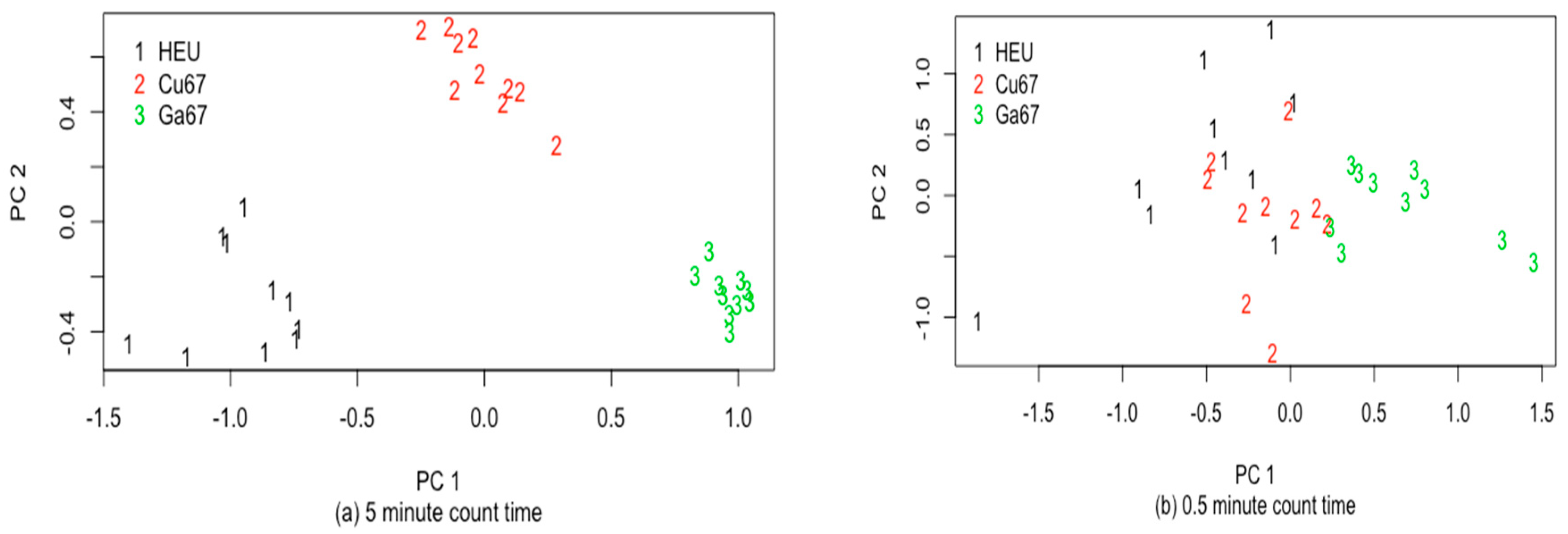
Another important isotope to recognize is U-235, whose spectrum can be confused with a few other isotopes, such as Cu-67 or Ga-67 because of nearby strong peaks as seen in Figure 13 in the low energy region. Figure 14a plots PC2 versus PC1 calculated from each of 10 simulated spectra from each of U-235 (indicated as HEU), Cu-67, and Ga-67 for a 5 min count time. Figure 14b is the same, but with a 0.5 min count time and item-specific model bias added as described above.
For 1000 test cases of each of U-235, Cu-67, and Ga6-7, the Figure 13 spectra lead to 100% correct classification in the Figure 14a case (5 min count time and no model bias). For 1000 test cases of each of U-235, Cu-67, and Ga-67, the Figure 13 spectra lead to 90% correct classification in the 14b case (0.5 min count time and model bias) and an average confidence (probability that the guessed group is correct) was also 90%, indicating good ABC calibration. For the 1000 test U-235 cases, 895 were predicted to be U-235, 103 were predicted to be Cu-67, and 2 were predicted to be Ga-67. The scaled count rate in each of 20 equally spaced energy bins were used as summary statistics (peak areas were not explicitly extracted), and there has not yet been an attempt to optimize performance by experimenting with candidate summary statistics, because all of the example RIID applications are for illustration only.
7. Discussion and Summary
A new ABC-based RIID was developed. The results show that the ABC-based RIID is well calibrated and that ABC is effective for inferring peak location, width, and area, which are key steps in peak-based RIID algorithms. It is important to recall that the simulated spectra are clearly distinct from the corresponding real spectra. Therefore, the forward model used in ABC, such as that in GADRAS [21] or that in Equation (1), has model bias that was addressed by comparing real to simulated spectra. More comparison of real to simulated spectra should be a next step. As real experiments with RIIDs become more costly, simulated data are likely to be more extensively used. Recall that already in practice, one quality check used by some RIIDs is whether simulated data agree reasonably well with the observed data; if so, there is reasonable confidence that the inferred subset is at least close to correct. However, simulation model bias is not yet considered in any existing fielded RIID to our knowledge. Future work will also adapt ABC for use with peak ratios as in [8] and will explore candidate summary statistics for ABC as in [8].
The RIID results in [8] relied on the simulated gamma library from [31]. Similarly, the RIID results in [9] were largely based on simulated data that were used to train a convolutional neural network using moderate resolution gamma detectors. It is likely that the simulated spectra in [9,31] are also distinct from the corresponding real spectra. However, the challenge problems in [8,9] were not difficult because the library isotopes (isotopes) were well separated (and so were the energy peaks), as were the isotopes analyzed in this paper. Simulation quality appears to be adequate in some situations, such as that in [8,9] and in the simple example in Section 6 summarized in Figure 10 where both groups 1 and 3 (Lu177m) are distinct from groups 2 and 4 (WgPu). Another remaining challenge is to assess to what extent RIID results on simulated data can be used to infer RIID performance on the corresponding real data [9].
Author Contributions
T.B. analyzed the data and developed the ABC applications. A.F., M.L. and J.S. simulated the spectra and collected the real data. All authors contributed to planning and writing the paper. All authors have read and agreed to the published version of the manuscript.
Funding
This research was funded by [Los Alamos National Laboratory] grant number [US DOE 89233218CNA000001] and the APC was funded by [Los Alamos National Laboratory].
Acknowledgments
Research reported in this publication was supported by the LANL Laboratory Directed Research and Development (LDRD) program at Los Alamos National Laboratory.
Conflicts of Interest
The authors declare no conflict of interest.
References
- Stromswold, D.; Carkoch, J.; Ely, J.; Hansen, R.; Kouzes, R.; Milbath, B.; Runkle, R.; Sliger, W.; Smart, J.; Stephens, D.; et al. Field Tests of a NaI(T1)-Based Vehicle Portal Monitor at Border Crossings. In Proceedings of the IEEE Nuclear Science Symposium Conference, Rome, Italy, 16–22 October 2004; Volume 1, pp. 196–200. Available online: http://0-ieeexplore-ieee-org.brum.beds.ac.uk/iel5/9892/31433/01462180.pdf (accessed on 11 November 2014).
- Sullivan, C.; Garner, S.; Lombardi, M.; Butterfield, K.; Smith-Nelson, M. Evaluation of key detector parameters for isotope identification. In Proceedings of the IEEE Nuclear Science Symposium Conference Record, Honolulu, HI, USA, 26 October–3 November 2007; pp. 1181–1184. [Google Scholar]
- Estep, R.; McCluskey, C.; Sapp, B. The multiple isotope material basis set (MIMBS) method for isotope identification with low- and medium-resolution-ray detectors. J. Radioanal. Nucl. Chem. 2008, 276, 737–741. [Google Scholar] [CrossRef]
- Miko, D.; Estep, R.; Rawool-Sullivan, M. An innovative method for extracting isotopic information from low-resolution spectra. Nucl. Instrum. Methods Phys. Res. A 1999, 422, 433–437. [Google Scholar] [CrossRef] [Green Version]
- Estep, R.; Rawool-Sullivan, M.; Miko, D. A Method for correcting NaI spectra for attenuation losses in hand-held instrument applications. IEEE Trans. Nucl. Sci. 1998, 45, 1022–1028. [Google Scholar] [CrossRef]
- Russ, W. Library correlation isotope identification algorithm. Nucl. Instrum. Methods Phys. Res. A 2007, 579, 288–291. [Google Scholar] [CrossRef]
- Burr, T.; Hamada, M. Radio-isotope identification algorithms for NaI gamma spectra. Algorithms 2009, 2, 339–360. [Google Scholar] [CrossRef] [Green Version]
- Sullivan, C.; Stinnett, J. Validation of a Bayesian-based isotope identification algorithm. Nucl. Instrum. Methods Phys. Res. A 2015, 784, 298–305. [Google Scholar] [CrossRef]
- Daniel, G.; Limousin, O.; Maler, D.; Meuris, A. Automatic and real-time identification of radioisotopes in gamma-ray spectra: A new method base on convolutional neural network trained with synthetic data set. IEEE Trans. Nucl. Sci. 2020, 4, 644–653. [Google Scholar] [CrossRef]
- Bai, E.; Chan, K.; Eichinger, W.; Kump, P. Detection of radioisotopes from weak and poorly resolved spectra using Lasso and subsampling techniques. Radiat. Meas. 2011, 46, 1138–1146. [Google Scholar] [CrossRef]
- Li, F.; Gu, Z.; Ge, L.; Li, H.; Tang, X.; Lang, X.; Hu, B. Review of recent gamma spectrum unfolding algorithms and their application. Results Phys. 2019, 13, 102211. [Google Scholar] [CrossRef]
- Mitchell, D. ASEDRA Evaluation Final Report, Sandia National Laboratory Report 2008-6382. 2008. Available online: https://prod-ng.sandia.gov/techlib-noauth/access-control.cgi/2008/086382.pdf (accessed on 3 July 2020).
- LaVigne, E.; Sjoden, G.; Backiak, J.; Detwiler, R. Extraordinary improvement in scintillation detectors via post-processing with ASEDRA-solution to a 50-year-old problem. In Proceedings of the SPIE, Orlando, FL, USA, 18 March 2008. [Google Scholar]
- Zhang, W.; Zahringer, M.; Ungar, K.; Hoffman, I. Statistical analysis of uncertainties of peak identification and area calculation in particulate air-filter environment radioisotope measurements using the results of a comprehensive nuclear-test-ban treaty organization organized intercomparison. Appl. Radiat. Isot. 2008, 66, 1695–1701. [Google Scholar] [CrossRef]
- Robinson, S.; Kiff, S.; Ashbaker, E.; Bender, S.; Flumerfelt, E.; Salvitti, M.; Borgardt, J.; Woodring, M. Effects of high count rate and gain shift on isotope identification algoritms. In Proceedings of the IEEE Nuclear Science Symposium Conference Record, Honolulu, HI, USA, 26 October–3 November 2007; Volume 2, pp. 1152–1156. [Google Scholar]
- Blackadar, J. Automatic isotope identifier and their features. IEEE Sens. J. 2005, 5, 589–592. [Google Scholar] [CrossRef]
- Pibida, L.; Unterweger, M.; Karam, L. Evaluation of handheld radioisotope identifiers. J. Res. Natl. Inst. Stand. Technol. 2004, 109, 451–456. [Google Scholar] [CrossRef] [PubMed]
- Sood, A.; Gardner, R. A new Monte Carlo assisted approach to detector response functions. Nucl. Instrum. Methods Phys. Res. B 2004, 213, 100–104. [Google Scholar] [CrossRef] [Green Version]
- Li, Z.; Zhang, Y.; Sun, S.; Want, B.; Wei, L. A semi-empirical response function for gamma-ray of Scintillation detector based on physical interaction mechanism. arXiv 2019, arXiv:1407.0799. [Google Scholar]
- Meleshenkovskii, L.; Pauly, N.; Labeau, P. Determination of the uranium enrichment without calibration standards using a 500 mm3 CdZnTe room temperature detector with a hybrid methodology based on peak ratios method and Monte Carlo counting efficiency simulations. Appl. Radiat. Isot. 2019, 148, 277–289. [Google Scholar] [CrossRef]
- Mitchell, D. Detector Response and Analysis Software (GADRAS); Sandia Report SAND88-2519; Sandia National Laboratories: Albuquerque, NM, USA, 1988.
- Blum, M.; Nunes, M.; Prangle, D.; Sisson, S. A Comparative review of dimension reduction methods in Approximate Bayesian Computation. Stat. Sci. 2013, 28, 189–208. [Google Scholar] [CrossRef]
- Burr, T.; Hengartner, N.; Matzner-Lober, E.; Myers, S.; Rouviere, L. Smoothing Low Resolution NaI Spectra. IEEE Trans. Nucl. Sci. 2010, 57, 2831–2840. [Google Scholar] [CrossRef]
- Burr, T.; Hamada, M.; Hengartner, N. Impact of spectral smoothing on gamma radiation portal alarm probabilities. Appl. Radiat. Isot. 2011, 69, 1436–1446. [Google Scholar] [CrossRef]
- Burr, T.; Skurikhin, A. Selecting Summary Statistics in Approximate Bayesian Computation for Calibrating Stochastic Models. BioMed Res. Int. 2013, 2013, 210646. [Google Scholar] [CrossRef] [Green Version]
- Burr, T.; Krieger, T.; Norman, C. Approximate Bayesian Computation applied to metrology for nuclear Safeguards. ESARDA Bull. 2018, 57, 50–59. [Google Scholar]
- Talts, S.; Betancourt, M.; Simpson, D.; Vehtari, A.; Gelman, A. Validating Bayesian inference algorithms with simulation-based calibration. arXiv 2018, arXiv:1804.06788. [Google Scholar]
- Burr, T.; Sampson, T.; Vo, D. Statistical evaluation of FRAM-ray isotopic analysis data. Appl. Radiat. Isot. 2005, 62, 931–940. [Google Scholar] [CrossRef] [PubMed]
- R Core Team. R: A Language and Environment for Statistical Computing; R Foundation for Statistical Computing: Vienna, Austria, 2013; Available online: http://www.R-project.org/ (accessed on 13 September 2020).
- Mariscotti, M. A Method for automatic identification of peaks in the presence of background and its application to spectrum analysis. Nucl. Instrum. Methods Phys. Res. A 1967, 50, 309. [Google Scholar] [CrossRef]
- Kong, X. Advanced Adaptive Library for Gamma-Ray Spectrometers. Master’s Thesis, University of Illinois, Urbana-Champaign, Urbana, IL, USA, 2014. Available online: www.ideals.illinois.edu/handle/2142/49390 (accessed on 6 January 2020).
- Sullivan, C.; Martinez, M.; Garner, S. Wavelet analysis of NaI spectra. IEEE Trans. Nucl. Sci. 2006, 53, 2916–2922. [Google Scholar] [CrossRef]
- Nunes, M.; Prangle, D. abctools: An R package for Tuning Approximate Bayesian Computation Analyses. R J. 2016, 7, 189–205. [Google Scholar] [CrossRef] [Green Version]
- Carlin, B.; John, B.; Stern, H.; Rubin, D. Bayesian Data Analysis, 1st ed.; Chapman and Hall: London, UK, 1995. [Google Scholar]
- Naus, J. Approximations for distributions of scan statistics. J. Am. Stat. Assoc. 1982, 77, 177–183. [Google Scholar] [CrossRef]
- Croft, S.; Favalli, A.; Weaver, B.; Williams, B.; Burr, T.; Henzlova, D.; McElroy, R. A Critical Examination of Figure of Merit (FOM): Assessing the Goodness-of-Fit in Gamma/X-ray Peak Analysis. Los Alamos National Laboratory Report LAUR 15-27783. 2015. Available online: https://permalink.lanl.gov/object/tr?what=info:lanl-repo/lareport/LA-UR-15-27783 (accessed on 16 October 2020).
- Burr, T.; Croft, S.; Jarman, K.; Nicholson, A.; Norman, C.; Walsh, S. Improved uncertainty quantification in nondestructive assay for nonproliferation. Chemometrics 2016, 159, 164–173. [Google Scholar] [CrossRef]
Figure 1.
Simulated and real (smoothed) I-131 spectral data.

Figure 2.
Similar to Figure 1, but for 2 energy regions: simulated and real I-131 spectra in (a,b). The real data are background adjusted, but model bias remains, as seen in (c,d).
Figure 2.
Similar to Figure 1, but for 2 energy regions: simulated and real I-131 spectra in (a,b). The real data are background adjusted, but model bias remains, as seen in (c,d).

Figure 3.
Raw data and example fits to one peak or to two peaks.

Figure 4.
Raw data, smooth fit 1 and smooth fit 2 for U-235 spectrum.

Figure 5.
(a,b) fit one peak to one peak, and (c,d) fit one peak to two close peaks.

Figure 6.
The relative bias in model 1 and model 2.

Figure 7.
Example of simulated raw and smooth spectra with a single true peak at 183.3 keV.

Figure 8.
ABC-based (Approximate Bayesian Computation) estimate of the posterior probability density function (pdf) for peak location using raw and smoothed data.
Figure 8.
ABC-based (Approximate Bayesian Computation) estimate of the posterior probability density function (pdf) for peak location using raw and smoothed data.

Figure 9.
Simulated (smoothed) Lu177m and WgPu spectra in (a) and scaled to range from 0 to 1 in (b).
Figure 9.
Simulated (smoothed) Lu177m and WgPu spectra in (a) and scaled to range from 0 to 1 in (b).

Figure 10.
Principle coordinate plot obtained using multidimensional scaling applied to real and simulated spectra for Lu-177m and WgPu.
Figure 10.
Principle coordinate plot obtained using multidimensional scaling applied to real and simulated spectra for Lu-177m and WgPu.

Figure 11.
The ABC-based posterior probabilities for each of the 4 models (1–4) in Figure 10 using an ABC-based radioisotope identification (RIID) that uses nonparametric estimates of each detected peak’s net area as summary statistics. The four classes (real and simulated Lu-177m and WgPu) are easily distinguished in this simple example with only 4 classes. This figure of model probabilities is for only 1 test case for illustration.

Figure 12.
PC 2 versus PC1 for 5 common naturally occurring materials for (a) 5 min count time without variation in the detector response function (DRF) and (b) 0.5 min count time with item-specific variation in the model bias as described.
Figure 12.
PC 2 versus PC1 for 5 common naturally occurring materials for (a) 5 min count time without variation in the detector response function (DRF) and (b) 0.5 min count time with item-specific variation in the model bias as described.

Figure 13.
Spectra (scaled count rate) versus energy (keV) for U-235 (HEU), Cu-67, and Ga-67.

Figure 14.
PC 2 versus PC 1 for U-235 (HEU), Cu-67, and Ga-67 for (a) 5 min count time without model bias and (b) 0.5 min count time with item-specific variation in the model bias.
Figure 14.
PC 2 versus PC 1 for U-235 (HEU), Cu-67, and Ga-67 for (a) 5 min count time without model bias and (b) 0.5 min count time with item-specific variation in the model bias.


Table 1.
Confusion matrix for 50,000 test cases with 10,000 simulated in each of naturally occurring radioactive material (NORM) groups 1–5. The true group is in the column and the inferred group is in the row.
Table 1.
Confusion matrix for 50,000 test cases with 10,000 simulated in each of naturally occurring radioactive material (NORM) groups 1–5. The true group is in the column and the inferred group is in the row.
| Inferred/True | 1 | 2 | 3 | 4 | 5 |
|---|---|---|---|---|---|
| 1 | 8927 | 0 | 0 | 1 | 80 |
| 2 | 788 | 10,000 | 0 | 5 | 95 |
| 3 | 272 | 0 | 10,000 | 89 | 387 |
| 4 | 13 | 0 | 0 | 9873 | 1713 |
| 5 | 0 | 0 | 0 | 32 | 7725 |
Publisher’s Note: MDPI stays neutral with regard to jurisdictional claims in published maps and institutional affiliations. |
© 2020 by the authors. Licensee MDPI, Basel, Switzerland. This article is an open access article distributed under the terms and conditions of the Creative Commons Attribution (CC BY) license (http://creativecommons.org/licenses/by/4.0/).
Share and Cite
MDPI and ACS Style
Burr, T.; Favalli, A.; Lombardi, M.; Stinnett, J. Application of the Approximate Bayesian Computation Algorithm to Gamma-Ray Spectroscopy. Algorithms 2020, 13, 265. https://0-doi-org.brum.beds.ac.uk/10.3390/a13100265
AMA Style
Burr T, Favalli A, Lombardi M, Stinnett J. Application of the Approximate Bayesian Computation Algorithm to Gamma-Ray Spectroscopy. Algorithms. 2020; 13(10):265. https://0-doi-org.brum.beds.ac.uk/10.3390/a13100265
Chicago/Turabian StyleBurr, Tom, Andrea Favalli, Marcie Lombardi, and Jacob Stinnett. 2020. "Application of the Approximate Bayesian Computation Algorithm to Gamma-Ray Spectroscopy" Algorithms 13, no. 10: 265. https://0-doi-org.brum.beds.ac.uk/10.3390/a13100265
Note that from the first issue of 2016, this journal uses article numbers instead of page numbers. See further details here.