Model-Based Real-Time Motion Tracking Using Dynamical Inverse Kinematics

Abstract

This paper contributes towards the development of motion tracking algorithms for time-critical applications, proposing an infrastructure for dynamically solving the inverse kinematics of highly articulate systems such as humans. The method presented is model-based, it makes use of velocity correction and differential kinematics integration in order to compute the system configuration. The convergence of the model towards the measurements is proved using Lyapunov analysis. An experimental scenario, where the motion of a human subject is tracked in static and dynamic configurations, is used to validate the inverse kinematics method performance on human and humanoid models. Moreover, the method is tested on a human-humanoid retargeting scenario, verifying the usability of the computed solution in real-time robotics applications. Our approach is evaluated both in terms of accuracy and computational load, and compared to iterative optimization algorithms.

1. Introduction

Nowadays, real-time motion tracking has many established applications in different fields such as medicine, virtual reality, and computer gaming. Moreover, in the field of robotics there is a growing interest in human motion retargeting and imitation [1,2]. Different tracking technologies and algorithms are currently available. Among these, optical tracking techniques are more spread and have been available since the 1980s [3]. Inertial/magnetic tracking technologies have been available only with the advent of micromachined sensors, and ensure higher frequency of data and lower latency, that makes them suited for demanding real-time motion tracking applications [4,5]. The objective of motion tracking algorithms is to find the human configuration given a set of inertial measurements. Tracking algorithms can use human body representations with different levels of complexity, spacing from contours [6,7], stick figure [8,9], and volumes [10,11]. For some techniques it is not required to know a priori the shape of the model, and model identification is part of the algorithm [6,8]. When the human is modeled as a kinematic chain, the solution of the model inverse kinematics has a major role in the algorithm [12,13,14,15], hence, strategies to solve it efficiently are required.

In the field of robotics, a common inverse kinematics problem consists in finding the mapping between the end-effector of a manipulator (task space) and the corresponding joint angles (configuration space). Compared to industrial manipulators, solving the inverse kinematics for a human kinematic model can be demanding as humans can be modelled as highly articulate kinematic chains. Human kinematics is redundant, it generally has a high number of degrees of freedom (DoF), and it should also take into account musculoskeletal constraints in order to ensure realistic motion. Moreover, a human moving in the space is a floating base system, which means that the configuration space lies on a differentiable manifold [16].

Since finding an analytical closed-form solution for the inverse kinematics of a human model is not always either possible or efficient, a numerical solution is often preferred. One of the most common approaches for solving inverse kinematics consists in formulating the problem as a non-linear optimization problem, that can be solved via iterative algorithms [17,18]. This class of algorithms can be referred to as instantaneous optimization since they aim to converge to a stable solution instantaneously at each time step. Although instantaneous optimization algorithms can converge fast to a solution in common robotics applications, the capability of finding an accurate solution for a human model, at a sufficient rate, can still be the bottleneck for some time-critical applications. However, there are many examples in which optimization is used for offline processing [19,20]. In some cases, better performances are achieved using heuristic iterative algorithms [21], learning algorithms [22], or combining analytical and numerical methods [23]. An alternative approach consists of embedding the static non-linear inverse kinematics problem into a dynamical one [24,25,26]. In order to underline the fact that, with this approach, a dynamic solution to the problem is found, we will refer to it as dynamical inverse-kinematics optimization. Note that this approach has been presented in literature also with other names such as motion rate control [27] and closed-loop inverse kinematics [28]. In practice, with this approach, the inverse kinematics problem is rephrased as a control problem, aiming to control the model configuration in order to converge to the sensors measurements. From a computational point of view, the main advantage of this approach is the fact that the solution can be computed directly at each time-step with a single iteration. The absence of iterations makes the dynamical optimization approach faster, therefore suitable for solving whole-body inverse kinematics of complex models in time-critical motion tracking applications. In literature, dynamical inverse kinematics has been successfully applied in real-time applications involving human or humanoid models [29,30].

This article presents a scheme for real-time motion tracking of highly articulate human, or humanoid, models. The tracking is achieved at a high frequency through a dynamic inverse kinematics optimization approach. The main contributions of this work are the application of a dynamical inverse kinematics strategy using rotation matrix parametrization for the rotation targets of the floating base human model, proving the convergence of the method using Lyapunov theory, and presenting a constrained inverse differential kinematic strategy to enforce model kinematic constraints. The implementation of the proposed scheme is tested for both human and humanoid models. The tests are preformed during different tasks involving both static posture and dynamic motions such as shown in Figure 1. The performances obtained using the dynamical inverse kinematics scheme are compared to the results obtained using instantaneous optimization methods. Further tests are performed using a real humanoid robot, controlling it in real-time using input sensors measurements and output of the humanoid model inverse kinematics. The paper is organized as follows: Section 2 introduces the notation, human modeling, formulation of motion tracking as an inverse kinematics problem, and the dynamical optimization scheme. Section 3 presents the proposed implementation of the dynamical inverse kinematics with rotation matrix parametrization and constrained inverse differential kinematics. In Section 4 the experimental details lay, and in Section 5 the performances are discussed and compared to instantaneous optimization. Conclusions follow in Section 6.

2. Background

2.1. Notation

• $\mathcal{I}$ denotes an inertial frame of reference.
• $I_{n\times n}\in {\mathbb{R}}^{n\times n}$ denotes the identity matrix of size n.
• ${{}^{\mathcal{A}}p}_{\mathcal{B}}\in {\mathbb{R}}^3$ is the position of the origin of the frame $\mathcal{B}$ with respect to the frame $\mathcal{A}$.
• ${{}^{\mathcal{A}}R}_{\mathcal{B}}\in SO\left(3\right)$ represents the rotation matrix of the frames $\mathcal{B}$ with respect to $\mathcal{A}$.
• ${{}^{\mathcal{A}}\omega }_{\mathcal{B}}\in {\mathbb{R}}^3$ is the angular velocity of the frame $\mathcal{B}$ with respect to $\mathcal{A}$, expressed in $\mathcal{A}$.
• The operator $\mathrm{tr}\left(·\right):{\mathbb{R}}^{3\times 3}\to \mathbb{R}$ denotes the trace of a matrix, such that given $A\in {\mathbb{R}}^{3\times 3}$, it is defined as $\mathrm{tr}\left(A\right):=A_{1,1}+A_{2,2}+A_{3,3}$.
• The operator $\mathrm{sk}\left(·\right):{\mathbb{R}}^{3\times 3}\to so\left(3\right)$ denotes skew-symmetric operation of a matrix, such that given $A\in {\mathbb{R}}^{3\times 3}$, it is defined as $\mathrm{sk}\left(A\right):=(A-A^{\top })/2$.
• The operator $S\left(·\right):{\mathbb{R}}^3\to so\left(3\right)$ denotes skew-symmetric vector operation, such that given two vectors $v,u\in {\mathbb{R}}^3$, it is defined as $v\times u=S\left(v\right)u$.
• The vee operator $·{}^{\vee }:so\left(3\right)\to {\mathbb{R}}^3$ denotes the inverse of the skew-symmetric vector operator, such that given a matrix $A\in so\left(3\right)$ and a vector $u\in {\mathbb{R}}^3$, it is defined as $Au=A^{\vee }\times u$.
• The operator ${∥·∥}_2$ indicates the L2-norm of a vector, such that given a vector $v\in {\mathbb{R}}^3$, it is defined as ${∥v∥}_2=\sqrt{v_1^2+v_2^2+v_3^2}$.

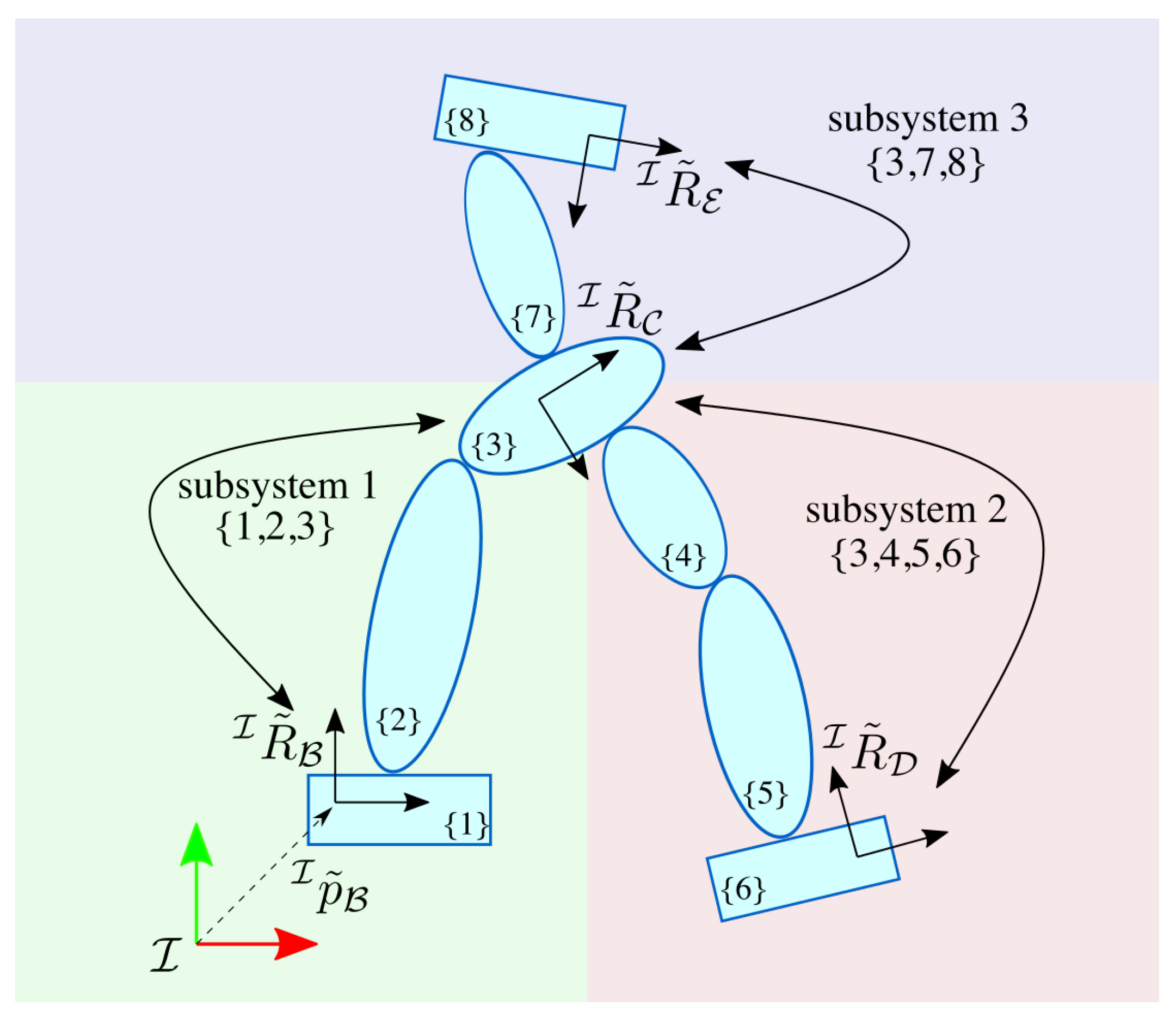
2.2. Modeling

The human is modeled as a multi-body mechanical system composed of $n+1$ rigid bodies, called links, that are connected by n joints with one degree of freedom (DoF) each [31]. Additionally, the system is assumed to be floating base, i.e., none of the links has an a priori constant pose with respect to the inertial frame $\mathcal{I}$. Hence, a specific frame, attached to a link of the system, is referred to as the base frame, denoted by $\mathcal{B}$.

The model configuration is characterized by the position and the orientation of the base frame along with the joint positions. Accordingly, the configuration space lies on the Lie group $\mathbb{Q}={\mathbb{R}}^3\times SO\left(3\right)\times {\mathbb{R}}^n$. An element of the configuration space $q\in \mathbb{Q}$ is defined as the triplet $q=({{}^{\mathcal{I}}p}_{\mathcal{B}},{{}^{\mathcal{I}}R}_{\mathcal{B}},s)$ where ${{}^{\mathcal{I}}p}_{\mathcal{B}}\in {\mathbb{R}}^3$ and ${{}^{\mathcal{I}}R}_{\mathcal{B}}\in SO\left(3\right)$ denote the position and the orientation of the base frame, and $s\in {\mathbb{R}}^n$ denotes the joints configuration representing the topology, i.e. shape, of the mechanical system. The position and the orientation of a frame $\mathcal{A}$ attached to the model can be obtained via geometrical forward kinematic map $h_{\mathcal{A}}\left(·\right):\mathbb{Q}\to (SO\left(3\right)\times {\mathbb{R}}^3)$ from the model configuration. The forward kinematics can be decomposed into position, i.e., ${{}^{\mathcal{I}}p}_{\mathcal{A}}=h_{\mathcal{A}}^p\left(q\right)$, and orientation, i.e., ${{}^{\mathcal{I}}R}_{\mathcal{A}}=h_{\mathcal{A}}^o\left(q\right)$, maps.

The model velocity is characterized by the linear and the angular velocity of the base frame along with the joint velocities. Accordingly, the configuration velocity space lies on the group $\mathbb{V}={\mathbb{R}}^3\times {\mathbb{R}}^3\times {\mathbb{R}}^n$. An element of the configuration velocity space $\nu \in \mathbb{V}$ is defined as $\nu =({{}^{\mathcal{I}}\mathrm{v}}_{\mathcal{B}},\dot{s})$ where ${{}^{\mathcal{I}}\mathrm{v}}_{\mathcal{B}}=({{}^{\mathcal{I}}\dot{p}}_{\mathcal{B}},{{}^{\mathcal{I}}\omega }_{\mathcal{B}})\in {\mathbb{R}}^3\times {\mathbb{R}}^3$ denotes the linear and angular velocity of the base frame, and $\dot{s}$ denotes the joint velocities. The velocity of a frame $\mathcal{A}$ attached to the model is represented as ${{}^{\mathcal{I}}\mathrm{v}}_{\mathcal{A}}=({{}^{\mathcal{I}}\dot{p}}_{\mathcal{A}},{{}^{\mathcal{I}}\omega }_{\mathcal{A}})$ where the two terms represent the linear and the angular velocity components respectively. The mapping between frame velocity ${{}^{\mathcal{I}}\mathrm{v}}_{\mathcal{A}}$ and configuration velocity $\nu$ is achieved through the Jacobian $J_{\mathcal{A}}=J_{\mathcal{A}}\left(q\right)\in {\mathbb{R}}^{6\times (n+6)}$, i.e., ${{}^{\mathcal{I}}\mathrm{v}}_{\mathcal{A}}=J_{\mathcal{A}}\left(q\right)\nu$. The Jacobian is composed of a linear part $J_{\mathcal{A}}^{\ell }\left(q\right)$ and an angular part $J_{\mathcal{A}}^a\left(q\right)$ mapping the linear and the angular velocities respectively, i.e., ${{}^{\mathcal{I}}\dot{p}}_{\mathcal{A}}=J_{\mathcal{A}}^{\ell }\left(q\right)\nu$ and ${{}^{\mathcal{I}}\omega }_{\mathcal{A}}=J_{\mathcal{A}}^a\left(q\right)\nu$.

2.3. Problem Statement

Motion tracking algorithms aim to find the model joint configuration given a set of targets describing the kinematics of the model links. The targets are the measurements of the link pose and velocity expressed in a world reference frame, and can be retrieved from various sensors measurements, e.g., processing of IMUs data [32]. The process of estimating the configuration of a mechanical system from task space measurements is generally referred to as inverse kinematics, and can be formulated as follows:

Problem 1.

Given a set of$n_p$frames$\mathcal{P}=\{{\mathcal{P}}_1,{\mathcal{P}}_2,\dots .{\mathcal{P}}_{n_p}\}$with the associated target position${{}^{\mathcal{I}}p}_{{\mathcal{P}}_i}\left(t\right)\in {\mathbb{R}}^3$and target linear velocity measurements${{}^{\mathcal{I}}\dot{p}}_{{\mathcal{P}}_i}\left(t\right)\in {\mathbb{R}}^3$, and given a set of$n_o$frames$\mathcal{O}=\{{\mathcal{O}}_1,{\mathcal{O}}_2,\dots .{\mathcal{O}}_{n_o}\}$with the associated target orientation${{}^{\mathcal{I}}R}_{{\mathcal{O}}_j}\left(t\right)\in SO\left(3\right)$and target angular velocity measurements${{}^{\mathcal{I}}\omega }_{{\mathcal{O}}_j}\left(t\right)\in {\mathbb{R}}^3$, and given the kinematic description of the model, find the state configuration ($q\left(t\right)$,$\nu \left(t\right)$) such that:

$$\left\{\begin{array}{cc}{{}^{\mathcal{I}}p}_{{\mathcal{P}}_i}\left(t\right)=h_{{\mathcal{P}}_i}^p\left(q\left(t\right)\right),\hfill & \forall i=1,\dots ,n_p\hfill \\ {{}^{\mathcal{I}}R}_{{\mathcal{O}}_j}\left(t\right)=h_{{\mathcal{O}}_j}^o\left(q\left(t\right)\right),\hfill & \forall j=1,\dots ,n_o\hfill \\ {{}^{\mathcal{I}}\dot{p}}_{{\mathcal{P}}_i}\left(t\right)=J_{{\mathcal{P}}_i}^{\ell }\left(q\left(t\right)\right)\nu \left(t\right),\hfill & \forall i=1,\dots ,n_p\hfill \\ {{}^{\mathcal{I}}\omega }_{{\mathcal{O}}_j}\left(t\right)=J_{{\mathcal{O}}_j}^a\left(q\left(t\right)\right)\nu \left(t\right),\hfill & \forall j=1,\dots ,n_o\hfill \\ A^{q}s\left(t\right)\le b^q,\hfill \\ A^{\nu }\dot{s}\left(t\right)\le b^{\nu },\hfill \end{array}\right.$$

(1)

where$A^q$and$b^q$are two constant parameters that represent the limits for model joints configuration, and$A^{\nu }$and$b^{\nu }$are two constant parameters that represent the limits for joint velocity.

The following quantities are defined in order to have a compact representation of Problem (1). The targets are collected in a pose target vector $x\left(t\right)$ and velocity target vector $\mathrm{v}\left(t\right)$:

$$x\left(t\right):=\left[\begin{array}{c}{{}^{\mathcal{I}}p}_{{\mathcal{P}}_1}\left(t\right)\\ ⋮\\ {{}^{\mathcal{I}}p}_{{\mathcal{P}}_{n_p}}\left(t\right)\\ {{}^{\mathcal{I}}R}_{{\mathcal{O}}_1}\left(t\right)\\ ⋮\\ {{}^{\mathcal{I}}R}_{{\mathcal{O}}_{n_o}}\left(t\right)\end{array}\right],\mathrm{v}\left(t\right):=\left[\begin{array}{c}{{}^{\mathcal{I}}\dot{p}}_{{\mathcal{P}}_1}\left(t\right)\\ ⋮\\ {{}^{\mathcal{I}}\dot{p}}_{{\mathcal{P}}_{n_p}}\left(t\right)\\ {{}^{\mathcal{I}}\omega }_{{\mathcal{O}}_1}\left(t\right)\\ ⋮\\ {{}^{\mathcal{I}}\omega }_{{\mathcal{O}}_{n_o}}\left(t\right)\end{array}\right],$$

(2)

while, forward geometrical kinematics and Jacobians are expressed respectively as a single vector $h\left(q\right(t\left)\right)$ and a single matrix $J\left(q\right(t\left)\right)$, such as:

$$h\left(q\left(t\right)\right):=\left[\begin{array}{c}{h}_{{\mathcal{P}}_1}^p\left(q\left(t\right)\right)\\ ⋮\\ h_{{\mathcal{P}}_{n_p}}^p\left(q\left(t\right)\right)\\ h_{{\mathcal{O}}_1}^o\left(q\left(t\right)\right)\\ ⋮\\ h_{{\mathcal{O}}_{n_o}}^o\left(q\left(t\right)\right)\end{array}\right],J\left(q\left(t\right)\right):=\left[\begin{array}{c}{J}_{{\mathcal{P}}_1}^{\ell }\left(q\left(t\right)\right)\\ ⋮\\ J_{{\mathcal{P}}_{n_p}}^{\ell }\left(q\left(t\right)\right)\\ J_{{\mathcal{O}}_1}^a\left(q\left(t\right)\right)\\ ⋮\\ J_{{\mathcal{O}}_{n_o}}^a\left(q\left(t\right)\right)\end{array}\right],$$

(3)

the set of equations in (1) can then be written compactly, using the definitions of (2) and (3), as the following two equations that describe the forward kinematics and differential kinematics respectively for all the target frames:

$$\begin{array}{cc}\hfill & x\left(t\right)=h\left(q\right(t\left)\right),\hfill \end{array}$$

(4a)

$$\begin{array}{cc}\hfill & \mathrm{v}\left(t\right)=J\left(q\right(t\left)\right)\nu \left(t\right).\hfill \end{array}$$

(4b)

As mentioned in Section 1, in the case of highly articulate systems, like humans, finding an analytical solution for the state configuration ($q\left(t\right)$,$\nu \left(t\right)$), satisfying the measurement Equations (4a) and (4b), is often not possible or too demanding. Hence, a numerical solution, such as non-linear optimization, is usually preferred (a general formulation of the non-linear optimization problem can be found in Section 5.1).

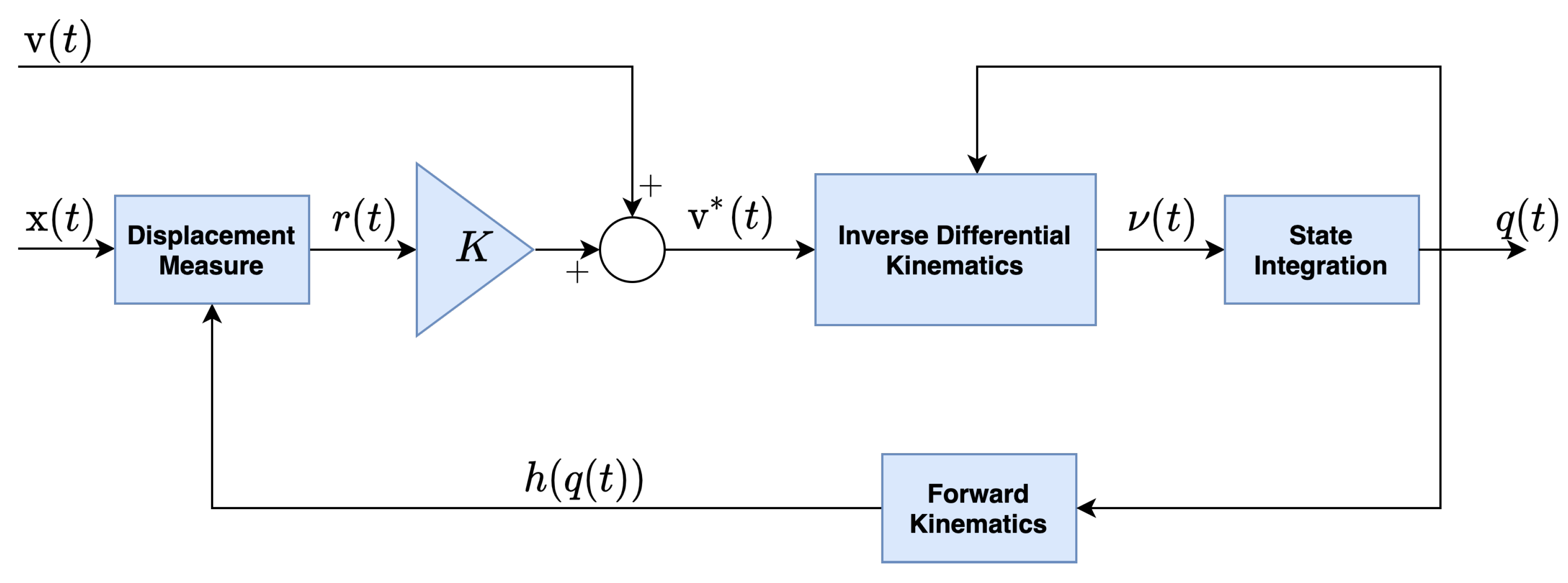
2.4. Dynamical Inverse Kinematics Optimization

Differently from instantaneous optimization methods, the dynamical optimization approach does not aim to satisfy the measurement Equations (4a) and (4b) at each time-step. Instead, the idea is to drive the state configuration ($q\left(t\right),\nu \left(t\right)$) to match the target measurements. In the language of control theory, the configuration velocity $\nu \left(t\right)$ is the control input, and the objective is to converge to the given target measurements. The block diagram for dynamical inverse kinematics implementation is presented in Figure 2. The scheme is designed in order to achieve the following three main tasks:

• correction of the measured velocity according to the current error,
• inversion of the model differential kinematics to compute the state velocity $\nu \left(t\right)$,
• integration of state velocity to compute the configuration $q\left(t\right)$.

The implementation of these three parts and the definition of the error are not unique, and depends on user design choices. In literature, Euler angles or unit quaternion parametrization are used for modeling floating base systems and for defining the rotational displacements. The implementation presented in the next section exploits rotation matrix parametrization both for target orientations and modeling of floating base systems. Moreover, a joint limit avoidance strategy is introduced in the inverse differential kinematics computation in order to comply with the model constraints. To the best of authors’ knowledge, the proposed scheme has not been used in literature before, with the presented implementation, for motion tracking applications.

3. Method

3.1. Velocity Correction Using Rotation Matrix

As a first instance, it is necessary to define some displacement measurements to be minimized. The displacements from the pose target vector $x\left(t\right)$, given the current state $q\left(t\right)$, are collected in a residual vector $r\left(q\right(t),x(t\left)\right)$ defined as follows:

$$r(q\left(t\right),x\left(t\right))=\left[\begin{array}{c}{{}^{\mathcal{I}}p}_{{\mathcal{P}}_1}\left(t\right)-h_{{\mathcal{P}}_1}^p\left(q\left(t\right)\right)\\ ⋮\\ \\ {{}^{\mathcal{I}}p}_{{\mathcal{P}}_{n_p}}\left(t\right)-h_{{\mathcal{P}}_{n_p}}^p\left(q\left(t\right)\right)\\ \mathrm{sk}{\left(h_{{\mathcal{O}}_1}^o{\left(q\left(t\right)\right)}^T{{}^{\mathcal{I}}R}_{{\mathcal{O}}_1}\left(t\right)\right)}^{\vee }\\ ⋮\\ \mathrm{sk}{\left(h_{{\mathcal{O}}_{n_o}}^o{\left(q\left(t\right)\right)}^T{{}^{\mathcal{I}}R}_{{\mathcal{O}}_{n_o}}\left(t\right)\right)}^{\vee }\end{array}\right].$$

(5)

Note that the position displacement is measured as Euclidean distance, while, the displacement between two orientation measurements is computed on SO(3) using rotation matrices with the $\mathrm{sk}{(.)}^{\vee }$ operator. The displacements from the target velocities $\mathrm{v}\left(t\right)$ are collected in the velocity residual vector $u\left(q\right(t),\nu (t),\mathrm{v}(t\left)\right)$. In this case all the vectors lie in a space over $\mathbb{R}$, and the residual vector is defined as:

$$u\left(q\right(t),\nu (t),\mathrm{v}(t\left)\right)=\mathrm{v}\left(t\right)-J\left(q\right(t\left)\right)\nu \left(t\right).$$

(6)

At this stage, we assume the state velocity $\nu \left(t\right)$ being the control input of a dynamical system described by the differential Equations (5) and (6), where we want to control the output residual vectors $r\left(t\right)$ and $u\left(t\right)$ to be driven to zero. As a consequence of the orientation error properties presented in [33], the following result holds.

Corollary 1.

Assume$r\left(q\right(t),x(t\left)\right)$defined as in (5),$u\left(q\right(t),\nu (t),\mathrm{v}(t\left)\right)$defined as in (6), and the system

$$u\left(q\right(t),\nu (t),\mathrm{v}(t\left)\right)+Kr\left(q\right(t),x(t\left)\right)=0,$$

(7)

where$K\in {\mathbb{R}}^{(3n_p+3n_o)}\times {\mathbb{R}}^{(3n_p+3n_o)}$is a positive definite diagonal matrix. Then,$(r,u)=(0,0)$denotes an (almost) globally asymptotically stable equilibrium point for the system.

The proof is provided in Appendix A. Corollary 1 shows that we can control the system so that $r\left(t\right)$ and $u\left(t\right)$ converge to zero for (almost) any initialization $q\left(t_0\right)$. The rate of convergence depends on the magnitude of the elements of matrix K, higher values of K imply faster convergence of the system (7) towards zero. Replacing the expression of $u\left(q\right(t),\nu (t\left)\right)$ presented in (6), into the system (7), we can derive an expression that is linear in the control input, i.e., state velocity $\nu \left(t\right)$:

$$J\left(q\right(t\left)\right)\nu \left(t\right)=\mathrm{v}\left(t\right)+Kr\left(q\right(t),x(t\left)\right).$$

(8)

The control input $\nu \left(t\right)$ can be obtained from Equation (8), the strategy to compute it will be the topic of the following Section 3.2.

Remark 1.

The existence of a solution for Equation (8) depends on the rank of the Jacobian matrix$J\left(q\right(t\left)\right)$, and of the augmented matrix$\left[J\right(q\left(t\right)\left)\right|\left(\mathrm{v}\right(t)+Kr(q\left(t\right),x\left(t\right)\left)\right)]$, there are many cases in which the solution can be found only numerically as a least-squares optimization. The presence of the optimization residual error ε, such that$J\left(q\right(t\left)\right)\nu \left(t\right)=\mathrm{v}\left(t\right)+Kr\left(q\right(t),x(t\left)\right)+\epsilon$, prevents the direct application of Corollary 1. However, the system convergence is ensured within a neighbourhood of the origin that depends on${∥\epsilon ∥}_2$(which is minimized within the optimization problem). The proof of it is beyond the scope of this paper.

Remark 2.

The Lyapunov analysis leading to Equation (8) has been done considering continuous-time. Some further considerations have to be done for discrete-time implementation. The discrete control input$\nu \left(t_k\right)$is obtained by replacing Equation (8) with the following discrete-time equation:

$$J\left(q\left(t_{k-1}\right)\right)\nu \left(t_k\right)=\mathrm{v}\left(t_k\right)+Kr(q\left(t_{k-1}\right),x\left(t_k\right)).$$

(9)

Moreover, discrete time solution bounds the values of K depending on the sampling time [34]. In case the sampling time is not constant, it might be opportune to use a variable gain$K=K\left(t_k\right)$.

According to the scheme in Figure 2, we will define a corrected velocity the term ${\mathrm{v}}^{*}\left(t_k\right)=\mathrm{v}\left(t_k\right)+Kr(q\left(t_{k-1}\right),x\left(t_k\right))$ that is used in inverse differential kinematics. The name underline the fact that the measured velocity $\mathrm{v}\left(t_k\right)$ is not used directly, but it is corrected proportionally to a residual error vector $r(q\left(t_{k-1}\right),x\left(t_k\right))$.

3.2. Constrained Inverse Differential Kinematics

The inverse differential kinematics is the problem of inverting the differential kinematics presented in Equation (4b) in order to find the configuration state velocity $\nu \left(t\right)$ for a given set of task space velocities. In order to compute the control input $\nu \left(t_k\right)$ from (9), it is required to solve the inverse differential kinematics for the corrected velocity vector ${\mathrm{v}}^{*}\left(t_k\right)$. Different strategies to solve the inverse differential kinematics can be found in literature [17,18,35,36], among the possible solutions, the most common approach is to use Jacobian generalized inverse [37]. In order to take into account also the model constraints, however, a Quadratic Progamming (QP) solver is preferred since it allows to introduce a set of constraints to the problem [38]. Hence, the inverse differential kinematics solution can be defined as the following QP optimization problem:

$$\begin{array}{ccc}\hfill & \underset{\nu \left(t_k\right)}{\mathrm{minimize}}\hfill & \hfill {∥{\mathrm{v}}^{*}\left(t_k\right)-J\left(q\left(t_{k-1}\right)\right)\nu \left(t_k\right)∥}_2\end{array}$$

(10a)

$$\begin{array}{ccc}\hfill & \mathrm{subject}\mathrm{to}\hfill & \hfill G\dot{s}\left(t_k\right)\le g.\end{array}$$

(10b)

While the joint velocities constraints can be used in the Equation (10b), joint position constraints, of the form

$$As\left(t_k\right)\le b^q,$$

(11)

can not be directly enforced in (10b) since they are independent from joint velocities $\dot{s}\left(t_k\right)$. For this reason, we propose a strategy that aims at converting joint space constraints (11) to velocity constraints such as (10b).

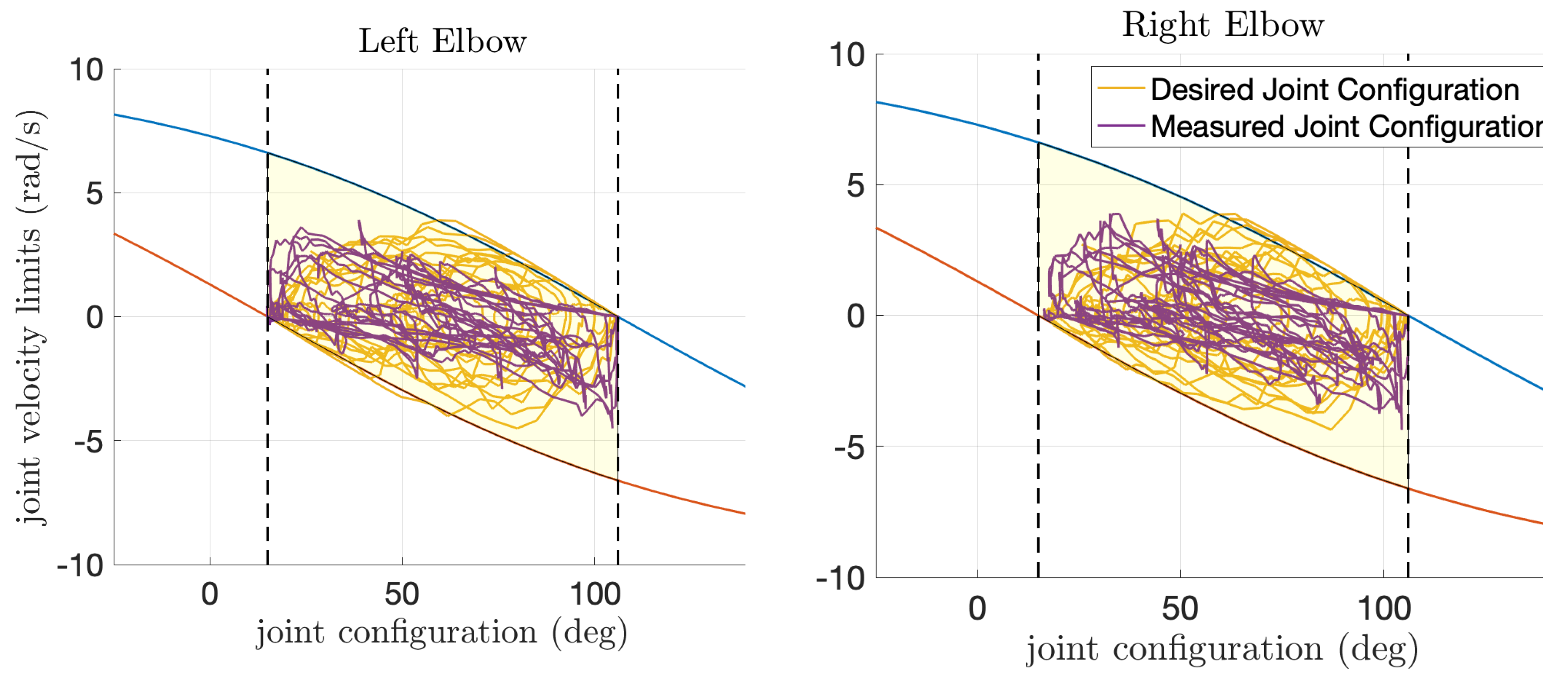
3.2.1. Joint Limit Avoidance

We start considering the simple case where we want to constraint a 1-DoF joint within its position limits $p_{min}\le p\le p_{max}$, and for which we define also a maximum and minimum velocity ${\dot{p}}_{min}\le \dot{p}\le {\dot{p}}_{max}$. In order to write all the constraints as velocity constraints, the idea is to limit the joint velocity as the position gets closer to its limits. This behaviour can be modelled using the hyperbolic tangent function, and defining the velocity limits as:

$$\tan \mathrm{h}\left(k_g^{min}(p-p_{min})\right){\dot{p}}_{min}\le \dot{p}\le \tan \mathrm{h}\left(k_g^{max}(p_{max}-p)\right){\dot{p}}_{max}.$$

(12)

where $k_g^{min}$ and $k_g^{max}$ are positive gains regulating the slope of the hyperbolic tangent, and $\tan \mathrm{h}\left(·\right)$ indicates the hyperbolic tangent function. When the joint is far from its limit, the argument of $\tan \mathrm{h}(.)$ is positive and far from zero, hence the hyperbolic tangent is $\approx 1$ and Equation (12) simply express the velocity limits. Instead, when the joint approaches the limits, the hyperbolic function goes to zero bounding the joint velocity to be positive, when approaching the lower joint limit, and negative when approaching the upper joint limit.

3.2.2. Linear Joint Space Constraints

Considering a set of joint space linear constraints, as defined in Equation (11), and following the 1-DoF example in Section 3.2.1, we can define dynamically the velocity constraint matrices, in Equation (10b), as

$$\begin{array}{cc}\hfill & G=A\hfill \end{array}$$

(13a)

$$\begin{array}{cc}\hfill & g=\tan \mathrm{h}\left(K_g(b^q-As)\right)\circ b^{\nu }.\hfill \end{array}$$

(13b)

where $K_g$ is a positive definite diagonal matrix, the operator ∘ indicates the element-wise multiplication, and $\tan \mathrm{h}\left(·\right)$ indicates the element-wise hyperbolic tangent function for a vector of scalars.

Remark 3.

It can happen that there is not a one-to-one mapping between the position constraints$(A^q,b^q)$and the velocity constraints$(A^{\nu },b^{\nu })$. In this case it is required to augment the constraint matrices by adding infinite constraints$b_i^q\to \infty$and$b_i^{\nu }\to \infty$, that, in practice, can approximated numerically.

Figure 3 shows the effect of the proposed limit avoidance approach in constraining the joints configuration-velocity space. It is important to notice that, in general, although the velocity is bounded to zero when approaching the limits, a violation of the constraints is possible. This would depend on the value of the gain $K_g$, the integration method, and the integration step $\Delta t$. However, in case of constraint violation, the change of sign of the velocity limit forces the configuration to return inside the bounds.

3.3. Numerical Integration

Given the configuration velocity solution $\nu \left(t_k\right)$, it is possible to compute the state configuration $q\left(t_k\right)$ by defining an initial configuration $q\left(t_0\right)$ and integrating over time. Base position ${{}^{\mathcal{I}}p}_{\mathcal{B}}$ and joints configuration s lie in vector space over $\mathbb{R}$ for which most of the numerical integrations methods proposed in literature can be used [39]. The integration of the base angular velocity ${{}^{\mathcal{I}}\omega }_{\mathcal{B}}\left(t_k\right)$ is not trivial [40], and numerical integration errors can lead to the violation of the orthonormality condition [41] for the base orientation ${{}^{\mathcal{I}}R}_{\mathcal{B}}$. There are different schemes that successfully solve discrete angular velocity integration making use of quaternion representation [40]. Concerning rotation matrix representation, the orthonormality condition can be directly enforced using the Baumgarte stabilization [41], and avoiding change of representation. The convergence of ${{}^{\mathcal{I}}R}_{\mathcal{B}}\left(t_k\right)$ over $SO\left(3\right)$, in fact, is ensured computing the base orientation matrix dynamics ${{}^{\mathcal{I}}\dot{R}}_{\mathcal{B}}\left(t_k\right)\in {\mathbb{R}}^{3\times 3}$ as follows:

$$\begin{array}{cc}\hfill & A\left(t_{k-1}\right)=\frac{\rho }{2}({\left({{}^{\mathcal{I}}R}_{\mathcal{B}}{\left(t_{k-1}\right)}^T{{}^{\mathcal{I}}R}_{\mathcal{B}}\left(t_{k-1}\right)\right)}^{-1}-I_{3\times 3}),\hfill \end{array}$$

(14a)

$$\begin{array}{cc}\hfill & {{}^{\mathcal{I}}\dot{R}}_{\mathcal{B}}\left(t_k\right)={{}^{\mathcal{I}}R}_{\mathcal{B}}\left(t_{k-1}\right)(S\left({{}^{\mathcal{I}}\omega }_{\mathcal{B}}\left(t_k\right)\right)+A\left(t_{k-1}\right)),\hfill \end{array}$$

(14b)

where $\rho \in {\mathbb{R}}^{+}$ is the gain regulating the convergence towards the orthonormality condition, and $\Delta t_k=t_k-t_{k-1}$ is the integration time step. The advantage of obtaining the configuration $q\left(t_k\right)$ through integration of velocity $\nu \left(t_k\right)$ is that the two estimated quantities are directly related, and continuity of the state configuration is ensured.

4. Experiments

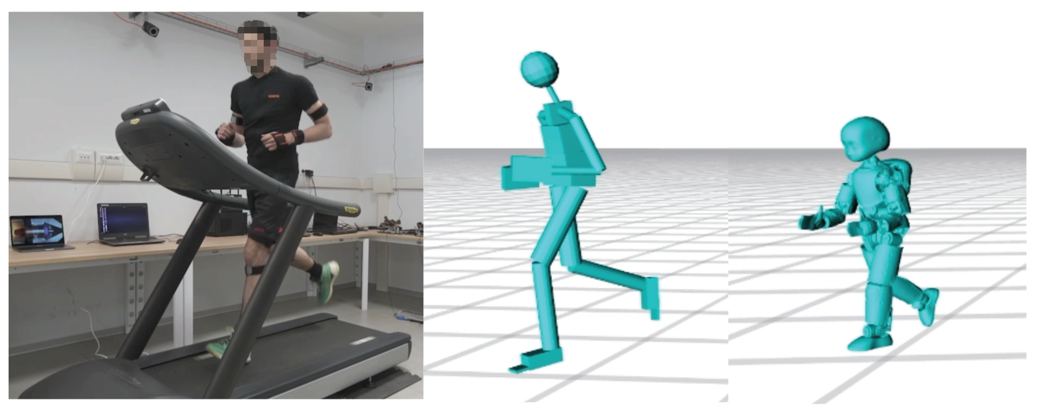
4.1. Motion Data Acquisition

The proposed method has been implemented and tested using motion data acquired with the Xsens Awinda wearable suit [42] providing pose and velocity of a 23 links human model, computed from a set of distributed Inertial Measurement Units (IMUs). The motion data is streamed through YARP middleware [43] that facilitates recording and real-time playback of data. The motion data is acquired for three scenarios with different levels of dynamicity: t-pose where the subject stands on two feet with the arms parallel to the ground, walking where the subject walks on a treadmill at a constant speed of $4 \mathrm{k}\mathrm{m}/\mathrm{h}$, and running where the subject runs on a treadmill at a constant speed of $10 \mathrm{k}\mathrm{m}/\mathrm{h}$.

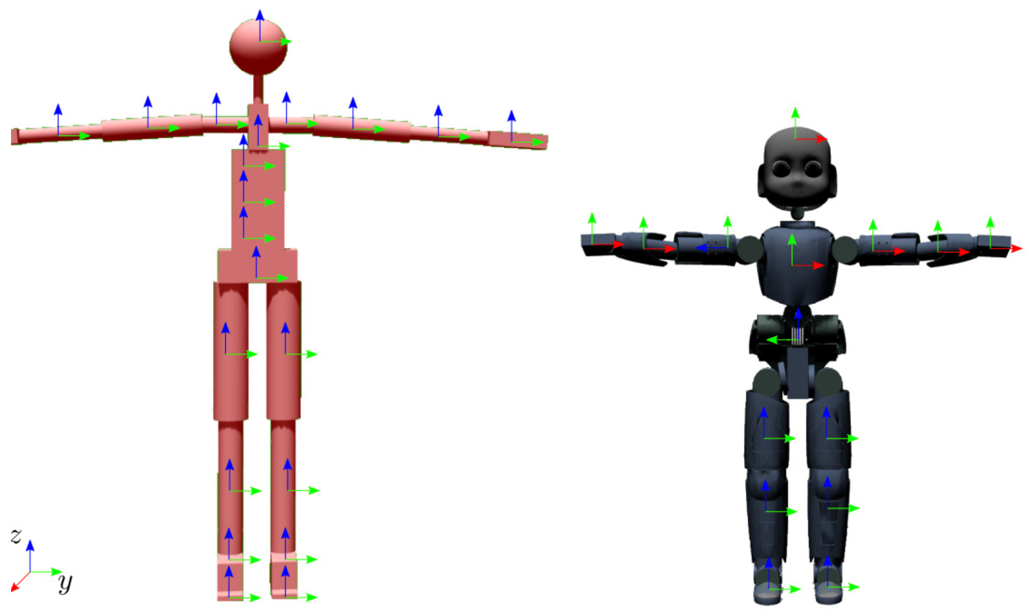
4.2. Models

The motion tracking is performed by using two different human models defined as in Section 2.2. Both the models are composed by 23 physical links representing segments of the human body. Each physical link is attached to the next one through a certain number of rotational joint connected through dummy links, i.e., links with dimension zero, in order to model human joints with multiple DoFs. In one human model (Human66) all the physical links are connected through spherical joints (3 rotational joints), i.e., a total of 66 DoFs and 67 links. The second model (Human48) is based on the modeling of the human musculoskeletal system as described in clinical studies [44,45,46], it has a reduced number of joint, i.e., 48DoFs, and takes into account human joint limits.

Additionally, we consider experiments with a model of the iCub humanoid robot [47]. The motivation behind this is to highlight the performance in achieving motion tracking, and motion retargeting from the human to a humanoid. The iCub model is composed of 15 physical links connected through 34 rotational joints. Model joint limits are defined according to the real robot mechanical constraints, including linear system of constraints involving multiple set of joints due to coupled joints mechanics.

The human https://github.com/robotology/human-gazebo and humanoid https://github.com/robotology/icub-models models are open-source resources. The definition of link frames for the human model and the robot model is highlighted in Figure 4. Considering that all the models have rotational joints only, the inverse kinematics problem is defined using rotational and angular velocity targets for each physical link, i.e., $n_o=23$ for the human model and $n_o=15$ for the humanoid model. Additionally, as both the models are floating base, a position and linear velocity target is used for the base frame, i.e., $n_p=1$.

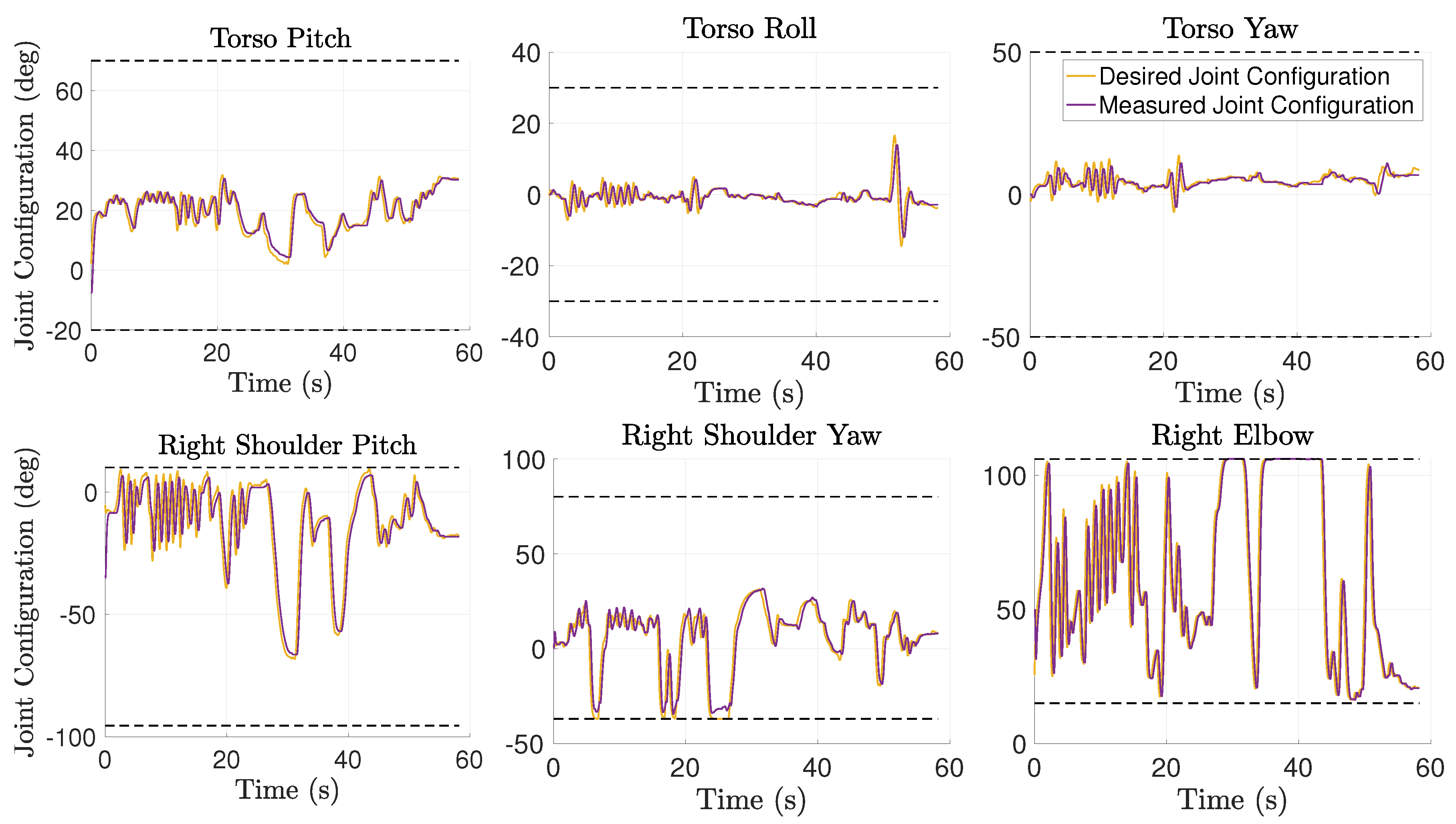
4.3. Robot Experiments

The iCub model inverse kinematics solution has been tested on the real robot in order to verify the feasibility of the computed configuration. The experimental setup involves an iCub robot fixed on a pole, as shown in Figure 5, controlled in position through low-level PID running at $1 \mathrm{k}\mathrm{Hz}$. The reference joint position is computed real-time using the dynamical inverse kinematics on the robot model, and the data are sent to the robot at the frequency of $50 \mathrm{Hz}$.

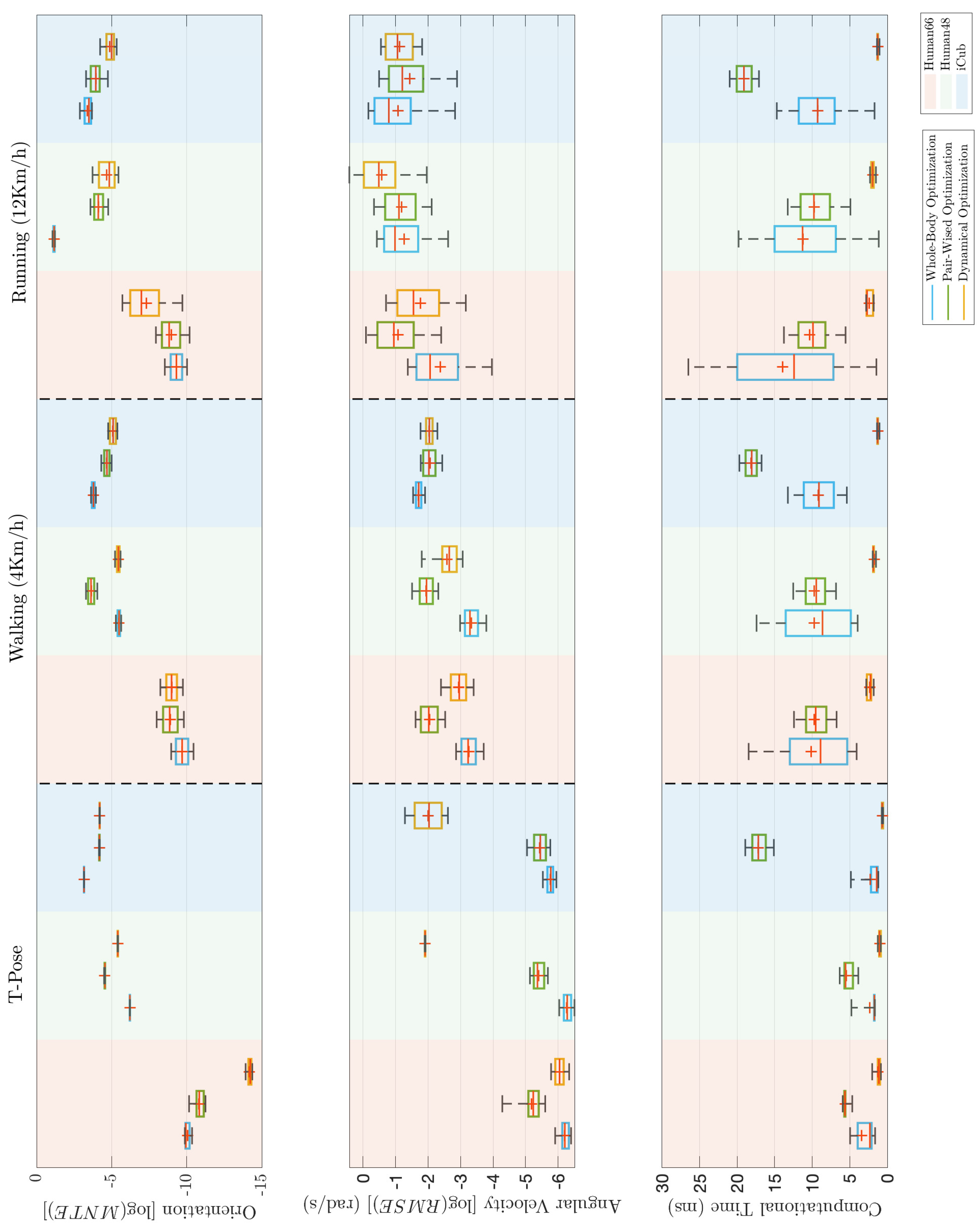
5. Results

The performance of dynamical optimization inverse kinematics solver is compared to instantaneous optimization implementations. The evaluation is done in terms of computational load and accuracy on a $2.3 \mathrm{G}\mathrm{Hz}$ Intel Core i7 processor with $16 \mathrm{GB}$ of RAM. The accuracy is measured with two metrics, one for the orientation targets and one for the velocity targets. The mean normalized trace error ($MNTE$) is a dimensionless metric measuring the overall accuracy of the orientation targets:

$$MNTE=\frac{1}{n_o}\sum _{j=1}^{n_o}\frac{\mathrm{tr}(I_{3\times 3}-h_{{\mathcal{O}}_j}^o{\left(q\right)}^T{{}^{\mathcal{I}}R}_{{\mathcal{O}}_j})}{2},$$

(15)

where the $\frac{1}{2}$ factor normalize the value of the trace between 0 and 1. For the angular velocities, the overall error is evaluated as root mean squared error ($RMSE$):

$$RMSE=\sqrt{\frac{1}{n_o}\sum _{j=1}^{n_o}\frac{{{∥{{}^{\mathcal{I}}\omega }_{{\mathcal{O}}_j}-{{}^{\mathcal{I}}\widehat{\omega }}_{{\mathcal{O}}_j}(q,\nu )∥}_2}^2}{3}},$$

(16)

where ${\widehat{\omega }}_{{\mathcal{O}}_j}(q,\nu )$ is the estimated frame velocity given the configuration $(q,\nu )$. The computational load is evaluated as the time for computing the state $(q,\nu )$. The statistics have been collected discarding the transient of 2 second from the initial time $t_0$.

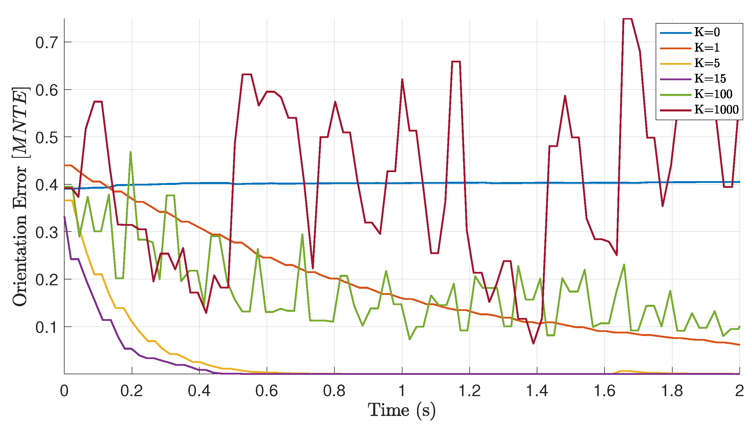
5.1. Instantaneous Optimization

As mentioned in Section 1, the instantaneous optimization methods solve the inverse kinematics at each time-step $t_k$ through non-linear optimization. A general formulation of the optimization problem is defined as follows:

$$\begin{array}{ccc}\hfill & \underset{q\left(t_k\right)}{\mathrm{minimize}}\hfill & \hfill {∥K_{r}r(q\left(t_k\right),x\left(t_k\right))∥}_2\end{array}$$

(17a)

$$\begin{array}{ccc}\hfill & \mathrm{subject}\mathrm{to}\hfill & \hfill As\left(t_k\right)\le b\end{array}$$

(17b)

where $K_r$ is a weight matrix that matches the unit measurements of target displacements, and eventually assigns a weight to each of the target. A common approach for solving the non-linear optimization problem is to consider the linear approximation of the system by recalling the Jacobian matrix definition, and solve the problem iteratively [48,49]. However, in order to enforce state configuration constraints, recent approaches make also use of convex optimization [36,50]. As benchmark, we have implemented instantaneous inverse kinematics optimization using iDynTree [51] multibody kinematics library, and the IPOPT software library for non-linear optimization [52]. The previous time-step solution has been used as warm-start for the non-linear optimizer, while the stopping criteria is the pose error accuracy and it has been tuned in order to find a solution in a time comparable to the dynamical optimization. Two different implementations have been tested. The former, referred to as whole-body optimization, solves a single optimization problem instantiated for the whole-system. The latter, instead, instantiates the optimization process dividing the model into multiple subsystems, each consisting of exactly a pair of targets, and solves the sub-problems in parallel. We refer to this implementation as pair-wise optimization. An example of model splitting for pair-wise optimization is shown in Figure 6.

Looking at Figure 7, it can be observed that the performance of instantaneous optimization approaches decreases as the task gets more dynamic. This is particularly evident for the computational time. In the whole-body optimization, the average computational time is higher, and it is characterized by a large variance, reaching peaks above $25$ ms during the running task. Concerning the pair-wised optimization, the increase of time between walking and running is less evident. However, the pair-wised optimization takes longer for finding a solution for the iCub model because of the local difference between the human and the robot kinematics.

5.2. Dynamical Optimization

The dynamical optimization inverse kinematics has been implemented using iDynTree multibody kinematics library [51], and the inverse differential kinematics is solved using OSQP [38]. Figure 8 highlights the rate of convergence of the error from a given initial zero configuration ($s\left(0\right)=0$) towards a target static pose. When the gain is zero, there is no velocity correction and the error remains constant. However, increasing the magnitude of K, the error converges to its steady state value in less than one second. A large value of the gain K leads to system instability as mentioned in Section 3.1.

From Figure 7, the dynamical optimization orientation error is mostly comparable with the results achieved with instantaneous optimization. The only case in which it shows worst orientation accuracy is with the Human66 model during running task. Concerning the angular velocity error, the performances are again comparable during dynamic motion, while it is higher for the T-pose with the constrained models. This angular velocity error may be due to the fact that a corrected angular velocity is used in place of the measured link angular velocities, and the joint constraints may introduce a constant constraint error because of an unfeasible configuration. Concerning the computational load, this method seems to outperform the others not only in terms of a mean computational time, having an average always below $3 \mathrm{m}\mathrm{s}$, but also for its consistency in different scenario.

Experiments with real-robot show the feasibility of the inverse kinematics solution. The robot is able to track real-time the motion of the human by following the computed joint configuration with a delay lower then $300 \mathrm{m}\mathrm{s}$, as shown in Figure 9 (evaluation of the controller is out of the scope of this work). Moreover, the joint limit avoidance strategy successfully constraints the joint angles within the robot physical limits that are never exceeded. More in details, Figure 3 shows the trajectory of some joints concerning both position and velocity, and it can be observed that the joint configuration remains within the joint constrained configuration space $(s,\dot{s})$.

6. Conclusions

This paper presents an infrastructure for whole-body inverse kinematics of highly articulated floating-base models in real-time motion tracking applications. The theory is presented using rotation matrix parametrization of orientations, together with the proof of convergence through Lyapunov analysis. The proposed method has been implemented and the performances tested in an experimental scenario with different conditions. Differently from iterative algorithms, the dynamical optimization requires a single iteration at each time step keeping the computational time constant, and ensures fast convergence of the error over time. Furthermore, the integration of velocities ensures obtaining a continuous and smooth solution. The method has been tested in a human-robot retargeting application to verify its usability. Its characteristics make it suitable for time-critical motion tracking applications with highly dynamic motions, where iterative algorithms may not converge in a sufficient time.

As a future work, the evaluation may be extended to a wider number of inverse kinematics algorithms, models, and experimental scenarios. Another interesting future work would be the extension of our method by considering the dynamics of the system as well.

References

- Dariush, B.; Gienger, M.; Arumbakkam, A.; Goerick, C.; Zhu, Y.; Fujimura, K. Online and markerless motion retargeting with kinematic constraints. In Proceedings of the 2008 IEEE/RSJ International Conference on Intelligent Robots and Systems, Nice, France, 22–26 September 2008; pp. 191–198. [Google Scholar] [CrossRef]
- Peng, X.B.; Abbeel, P.; Levine, S.; van de Panne, M. DeepMimic: Example-guided Deep Reinforcement Learning of Physics-based Character Skills. ACM Trans. Graph. 2018, 37, 143:1–143:14. [Google Scholar] [CrossRef] [Green Version]
- Aggarwal, J.K.; Cai, Q. Human motion analysis: A review. Comput. Vis. Image Underst. 1999, 73, 428–440. [Google Scholar] [CrossRef]
- Zhu, R.; Zhou, Z. A real-time articulated human motion tracking using tri-axis inertial/magnetic sensors package. IEEE Trans. Neural Syst. Rehabil. Eng. 2004, 12, 295–302. [Google Scholar] [CrossRef] [PubMed]
- Filippeschi, A.; Schmitz, N.; Miezal, M.; Bleser, G.; Ruffaldi, E.; Stricker, D. Survey of motion tracking methods based on inertial sensors: A focus on upper limb human motion. Sensors 2017, 17, 1257. [Google Scholar] [CrossRef] [PubMed] [Green Version]
- Shio, A.; Sklansky, J. Segmentation of people in motion. In Proceedings of the IEEE Workshop on Visual Motion, Princeton, NJ, USA, 7–9 October 1991; pp. 325–332. [Google Scholar] [CrossRef]
- Leung, M.K.; Yang, Y.-H. First Sight: A human body outline labeling system. IEEE Trans. Pattern Anal. Mach. Intell. 1995, 17, 359–377. [Google Scholar] [CrossRef]
- Niyogi, S.A.; Adelson, E.H. Analyzing and recognizing walking figures in XYT. In Proceedings of the 1994 IEEE Conference on Computer Vision and Pattern Recognition, Seattle, WA, USA, 21–23 June 1994; pp. 469–474. [Google Scholar] [CrossRef]
- Bharatkumar, A.G.; Daigle, K.E.; Pandy, M.G.; Cai, Q.; Aggarwal, J.K. Lower limb kinematics of human walking with the medial axis transformation. In Proceedings of the 1994 IEEE Workshop on Motion of Non-Rigid and Articulated Objects, Austin, TX, USA, 11–12 November 1994; pp. 70–76. [Google Scholar] [CrossRef]
- Wachter, S.; Nagel, H.H. Tracking persons in monocular image sequences. Comput. Vis. Image Underst. 1999, 74, 174–192. [Google Scholar] [CrossRef]
- Gall, J.; Stoll, C.; De Aguiar, E.; Theobalt, C.; Rosenhahn, B.; Seidel, H.P. Motion capture using joint skeleton tracking and surface estimation. In Proceedings of the 2009 IEEE Conference on Computer Vision and Pattern Recognition, Miami, FL, USA, 20–25 June 2009; pp. 1746–1753. [Google Scholar]
- Monzani, J.S.; Baerlocher, P.; Boulic, R.; Thalmann, D. Using an Intermediate Skeleton and Inverse Kinematics for Motion Retargeting; Computer Graphics Forum; Wiley Online Library: Oxford, UK, 2000; Volume 19, pp. 11–19. [Google Scholar]
- Pons-Moll, G.; Baak, A.; Gall, J.; Leal-Taixe, L.; Mueller, M.; Seidel, H.P.; Rosenhahn, B. Outdoor human motion capture using inverse kinematics and von mises-fisher sampling. In Proceedings of the 2011 International Conference on Computer Vision, Barcelona, Spain, 6–13 November 2011; pp. 1243–1250. [Google Scholar]
- Ganapathi, V.; Plagemann, C.; Koller, D.; Thrun, S. Real time motion capture using a single time-of-flight camera. In Proceedings of the 2010 IEEE Computer Society Conference on Computer Vision and Pattern Recognition, San Francisco, CA, USA, 13–18 June 2010; pp. 755–762. [Google Scholar]
- Aristidou, A.; Lasenby, J. Motion capture with constrained inverse kinematics for real-time hand tracking. In Proceedings of the 2010 4th International Symposium on Communications, Control and Signal Processing (ISCCSP), Limassol, Cyprus, 3–5 March 2010; pp. 1–5. [Google Scholar]
- Traversaro, S.; Saccon, A. Multibody Dynamics Notation; Tech. Rep.; Technische Universiteit Eindhoven: Eindhoven, The Netherlands, 2016. [Google Scholar]
- Goldenberg, A.; Benhabib, B.; Fenton, R. A complete generalized solution to the inverse kinematics of robots. IEEE J. Robot. Autom. 1985, 1, 14–20. [Google Scholar] [CrossRef]
- Buss, S.R. Introduction to inverse kinematics with jacobian transpose, pseudoinverse and damped least squares methods. IEEE J. Robot. Autom. 2004, 17, 16. [Google Scholar]
- Kok, M.; Hol, J.; Schön, T. An optimization-based approach to human body motion capture using inertial sensors. In Proceedings of the 19th World Congress of the International Federation of Automatic Control (IFAC), Cape Town, South Africa, 24–29 August 2014; pp. 79–85. [Google Scholar]
- Von Marcard, T.; Rosenhahn, B.; Black, M.J.; Pons-Moll, G. Sparse Inertial Poser: Automatic 3D Human Pose Estimation from Sparse Imus; Computer Graphics Forum; Wiley Online Library: Oxford, UK, 2017; Volume 36, pp. 349–360. [Google Scholar]
- Aristidou, A.; Lasenby, J. FABRIK: A fast, iterative solver for the Inverse Kinematics problem. Graph. Models 2011, 73, 243–260. [Google Scholar] [CrossRef]
- Grochow, K.; Martin, S.L.; Hertzmann, A.; Popović, Z. Style-based inverse kinematics. ACM Trans. Graph. (TOG) 2004, 23, 522–531. [Google Scholar] [CrossRef] [Green Version]
- Tolani, D.; Goswami, A.; Badler, N.I. Real-Time Inverse Kinematics Techniques for Anthropomorphic Limbs. Graph. Models 2000, 62, 353–388. [Google Scholar] [CrossRef] [Green Version]
- Sciavicco, L.; Siciliano, B. A dynamic solution to the inverse kinematic problem for redundant manipulators. In Proceedings of the 1987 IEEE International Conference on Robotics and Automation, Raleigh, NC, USA, 31 March–3 April 1987; Volume 4, pp. 1081–1087. [Google Scholar]
- Balestrino, A.; De Maria, G.; Sciavicco, L. Robust control of robotic manipulators. IFAC Proc. Vol. 1984, 17, 2435–2440. [Google Scholar] [CrossRef]
- Wolovich, W.A.; Elliott, H. A computational technique for inverse kinematics. In Proceedings of the 23rd IEEE Conference on Decision and Control, Las Vegas, NV, USA, 12–14 December 1984; pp. 1359–1363. [Google Scholar]
- Whitney, D.E. Resolved motion rate control of manipulators and human prostheses. IEEE Trans. Man-Mach. Syst. 1969, 10, 47–53. [Google Scholar] [CrossRef]
- Chiacchio, P.; Chiaverini, S.; Sciavicco, L.; Siciliano, B. Closed-loop inverse kinematics schemes for constrained redundant manipulators with task space augmentation and task priority strategy. Int. J. Robot. Res. 1991, 10, 410–425. [Google Scholar] [CrossRef]
- Andrews, S.; Huerta, I.; Komura, T.; Sigal, L.; Mitchell, K. Real-time physics-based motion capture with sparse sensors. In Proceedings of the 13th European Conference on Visual Media Production (CVMP 2016), London, UK, 12–13 December 2016; pp. 1–10. [Google Scholar]
- Suleiman, W.; Ayusawa, K.; Kanehiro, F.; Yoshida, E. On prioritized inverse kinematics tasks: Time-space decoupling. In Proceedings of the 2018 IEEE 15th International Workshop on Advanced Motion Control (AMC), Tokyo, Japan, 9–11 March 2018; pp. 108–113. [Google Scholar]
- Latella, C.; Lorenzini, M.; Lazzaroni, M.; Romano, F.; Traversaro, S.; Akhras, M.A.; Pucci, D.; Nori, F. Towards real-time whole-body human dynamics estimation through probabilistic sensor fusion algorithms. Auton. Robots 2019, 43, 1591–1603. [Google Scholar] [CrossRef] [Green Version]
- Kok, M.; Hol, J.D.; Schön, T.B. Using inertial sensors for position and orientation estimation. arXiv 2017, arXiv:1704.06053. [Google Scholar]
- Olfati-Saber, R. Nonlinear Control of Underactuated Mechanical Systems with Application to Robotics and Aerospace Vehicles. Ph.D. Thesis, Massachusetts Institute of Technology, Cambridge, MA, USA, 2001. [Google Scholar]
- Ogata, K. Discrete-Time Control Systems; Prentice Hall: Englewood Cliffs, NJ, USA, 1995; Volume 2. [Google Scholar]
- Sciavicco, L.; Siciliano, B. A solution algorithm to the inverse kinematic problem for redundant manipulators. IEEE J. Robot. Autom. 1988, 4, 403–410. [Google Scholar] [CrossRef]
- Kanoun, O.; Lamiraux, F.; Wieber, P. Kinematic Control of Redundant Manipulators: Generalizing the Task-Priority Framework to Inequality Task. IEEE Trans. Robot. 2011, 27, 785–792. [Google Scholar] [CrossRef] [Green Version]
- Rao, C.R.; Mitra, S.K. Generalized inverse of a matrix and its applications. In Proceedings of the Sixth Berkeley Symposium on Mathematical Statistics and Probability, Volume 1: Theory of Statistics; The Regents of the University of California: Berkeley, CA, USA, 1972. [Google Scholar]
- Stellato, B.; Banjac, G.; Goulart, P.; Bemporad, A.; Boyd, S. OSQP: An Operator Splitting Solver for Quadratic Programs. Math. Program. Comput. 2020. [Google Scholar] [CrossRef] [Green Version]
- Davis, P.J.; Rabinowitz, P. Methods of Numerical Integration; Courier Corporation: North Chelmsford, MA, USA, 2007. [Google Scholar]
- Boyle, M. The integration of angular velocity. Adv. Appl. Clifford Algebr. 2017, 27, 2345–2374. [Google Scholar] [CrossRef] [Green Version]
- Gros, S.; Zanon, M.; Diehl, M. Baumgarte stabilisation over the SO(3) rotation group for control. In Proceedings of the 2015 54th IEEE Conference on Decision and Control (CDC), Osaka, Japan, 15–18 December 2015; pp. 620–625. [Google Scholar] [CrossRef]
- Roetenberg, D.; Luinge, H.; Slycke, P. Xsens MVN: Full 6DOF Human Motion Tracking Using Miniature Inertial Sensors; Xsens Technologies B.V.: Enschede, The Netherlands, 2009. [Google Scholar]
- Metta, G.; Fitzpatrick, P.; Natale, L. YARP: yet another robot platform. Int. J. Adv. Robot. Syst. 2006, 3, 8. [Google Scholar] [CrossRef] [Green Version]
- Moll, J.; Wright, V. Normal range of spinal mobility. An objective clinical study. Ann. Rheum. Dis. 1971, 30, 381. [Google Scholar] [CrossRef] [PubMed] [Green Version]
- Gerhardt, J. Clinical measurements of joint motion and position in the neutral-zero method and SFTR recording: Basic principles. Int. Rehabil. Med. 1983, 5, 161–164. [Google Scholar] [CrossRef] [PubMed]
- Alison Middleditch, M.; Jean Oliver, M. Functional Anatomy of the Spine; Elsevier Health Sciences: Oxford, UK, 2005; ISBN 0-7506-2717-4. [Google Scholar]
- Natale, L.; Bartolozzi, C.; Pucci, D.; Wykowska, A.; Metta, G. icub: The not-yet-finished story of building a robot child. Sci. Robot. 2017, 2, eaaq1026. [Google Scholar] [CrossRef]
- Barnes, J. An algorithm for solving non-linear equations based on the secant method. Comput. J. 1965, 8, 66–72. [Google Scholar] [CrossRef] [Green Version]
- Fletcher, R. Generalized Inverse Methods for the Best Least Squares Solution of Systems of Non-Linear Equations. Comput. J. 1968, 10, 392–399. [Google Scholar] [CrossRef] [Green Version]
- Blanchini, F.; Fenu, G.; Giordano, G.; Pellegrino, F.A. A convex programming approach to the inverse kinematics problem for manipulators under constraints. Eur. J. Control 2017, 33, 11–23. [Google Scholar] [CrossRef] [Green Version]
- Nori, F.; Traversaro, S.; Eljaik, J.; Romano, F.; Del Prete, A.; Pucci, D. iCub Whole-body Control through Force Regulation on Rigid Noncoplanar Contacts. Front. Robot. AI 2015, 2, 6. [Google Scholar] [CrossRef] [Green Version]
- Wächter, A.; Biegler, L.T. On the implementation of an interior-point filter line-search algorithm for large-scale nonlinear programming. Math. Program. 2006, 106, 25–57. [Google Scholar] [CrossRef]
Publisher’s Note: MDPI stays neutral with regard to jurisdictional claims in published maps and institutional affiliations. |
© 2020 by the authors. Licensee MDPI, Basel, Switzerland. This article is an open access article distributed under the terms and conditions of the Creative Commons Attribution (CC BY) license (http://creativecommons.org/licenses/by/4.0/).
Share and Cite
Rapetti, L.; Tirupachuri, Y.; Darvish, K.; Dafarra, S.; Nava, G.; Latella, C.; Pucci, D. Model-Based Real-Time Motion Tracking Using Dynamical Inverse Kinematics. Algorithms 2020, 13, 266. https://0-doi-org.brum.beds.ac.uk/10.3390/a13100266
Rapetti L, Tirupachuri Y, Darvish K, Dafarra S, Nava G, Latella C, Pucci D. Model-Based Real-Time Motion Tracking Using Dynamical Inverse Kinematics. Algorithms. 2020; 13(10):266. https://0-doi-org.brum.beds.ac.uk/10.3390/a13100266
Chicago/Turabian StyleRapetti, Lorenzo, Yeshasvi Tirupachuri, Kourosh Darvish, Stefano Dafarra, Gabriele Nava, Claudia Latella, and Daniele Pucci. 2020. "Model-Based Real-Time Motion Tracking Using Dynamical Inverse Kinematics" Algorithms 13, no. 10: 266. https://0-doi-org.brum.beds.ac.uk/10.3390/a13100266