Similarity-Driven Edge Bundling: Data-Oriented Clutter Reduction in Graphs Layouts
by

Fabio Sikansi
1, 
Renato R. O. da Silva
1,
Gabriel D. Cantareira
1,
Elham Etemad
2 and
Fernando V. Paulovich
1,2,*
1
Instituto de Ciências Matemáticas e de Computação, Universidade de São Paulo, São Carlos, SP 13566-590, Brazil
2
Faculty of Computer Science, Dalhousie University, Halifax, NS B3H 4R2, Canada
*
Author to whom correspondence should be addressed.
Algorithms 2020, 13(11), 290; https://0-doi-org.brum.beds.ac.uk/10.3390/a13110290
Submission received: 26 September 2020
/
Revised: 6 November 2020
/
Accepted: 7 November 2020
/
Published: 10 November 2020
(This article belongs to the Special Issue Graph Drawing and Information Visualization)
Abstract
:Graph visualization has been successfully applied in a wide range of problems and applications. Although different approaches are available to create visual representations, most of them suffer from clutter when faced with many nodes and/or edges. Among the techniques that address this problem, edge bundling has attained relative success in improving node-link layouts by bending and aggregating edges. Despite their success, most approaches perform the bundling based only on visual space information. There is no explicit connection between the produced bundled visual representation and the underlying data (edges or vertices attributes). In this paper, we present a novel edge bundling technique, called Similarity-Driven Edge Bundling (SDEB), to address this issue. Our method creates a similarity hierarchy based on a multilevel partition of the data, grouping edges considering the similarity between nodes to guide the bundling. The novel features introduced by SDEB are explored in different application scenarios, from dynamic graph visualization to multilevel exploration. Our results attest that SDEB produces layouts that consistently follow the similarity relationships found in the graph data, resulting in semantically richer presentations that are less cluttered than the state-of-the-art.
1. Introduction
Graph visualization has been applied in a wide range of domains to model and support the analysis of different relationships between elements, from protein-protein interaction [1] and biomolecular relationships [2] to social networks [3]. Despite its popularity, effective graph visualization presents several challenges, especially when dealing with dense graphs with many vertices or edges [4,5]. In these scenarios, the visualizations usually present considerable overlapping of visual elements, resulting in cluttered layouts that make it hard or even impossible for users to extract relevant information.
Clutter reduction is a frequent subject in data visualization [6]. In general, it aims to reorganize or transform visual elements so that the attained representation can reveal meaningful patterns hidden in the original layout. Specifically for graph visualization techniques, Edge Bundling has obtained relative success in reducing visual clutter on node-link diagrams by bending and aggregating groups of edges [7,8,9]. Additionally, the curves’ smoothness also improves the visual representations making it easier to follow high-level edge patterns [10], allowing to produce layouts that support the overview of large graphs.
Over recent years, different edge bundling strategies have been proposed. the seminal technique, Hierarchical Edge Bundling (HEB) [11], employs an external hierarchical structure to guide the edges’ bending and, therefore, cannot be used if such a structure is not provided. Several approaches have been devised to address this limitation, avoiding the need for any other information besides graph adjacency and vertex positions. Some examples include strategies based on force-directed placement [10,12], geometry processing [13,14], clustering [15,16] and image processing [17,18,19]. Despite the high degree of clutter reduction these techniques can attain, they only use the visual space (graph embedding) to perform the edge bundling. So that resulting in aggregations that might not explicitly reflect the underlying data (edges or vertices attributes). Recently, the use of data information to guide the bundling gained attention [20,21,22,23], usually adapting existing techniques. However, only edge information is considered, ignoring information on the vertices, narrowing their applicability.
In this paper, we present Similarity-Based Edge Bundling (SBED), an adaptation of the HEB technique to construct bundling layouts that do not depend on an external hierarchy and consider similarity relationships among the vertices to add semantics to the bundled representations. Our approach uses a two-step process. On the first step, we derive a distance-preserving backbone structure to serve as a guide for the bundling, and, on the second, the straight edges are curved towards such a structure. Besides consistently representing the underlying data similarity relationships, a bonus of using this backbone is the possibility of multiscale visualization and exploration. Bundled layouts can be explored into different levels of detail, from coarser levels, better suited for exploring the main patterns between groups, to finer levels, supporting the exploration of intra-group relationships.
In summary, the main contributions of this paper are:
- An approach to creating graph bundling layouts in which the bundles are defined based on similarity relationships;
- A strategy to explore bundling layouts using a multiscale approach using aggregation and adaptative bundling parameters; and
- A stable strategy to bundle edges in graphs with time-varying topology.
In Section 2, we overview the more important graph edge bundling techniques, discussing their limitations. In Section 3, we explain the different strategies we develop to address the problem of creating bundled layouts that reflects the underlying data similarity, including the simplification procedure to allow multilevel navigation. In Section 4, we present a quantitative and qualitative analysis of the proposed strategies, comparing our results with the state-of-art in bundling techniques. In Section 5, we show how SDEB can be used in different scenarios, and we draw our conclusions in Section 7.
2. Related Work
Edge bundling is a well-known approach to reduce visual clutter in different information visualization techniques [7]. For the graph domain, the original idea was proposed by Holten [11] called Hierarchical Edge Bundling (HEB). HEB employs hierarchical data to settle paths to guide the bending and grouping of edges. This is performed, drawing each edge as a B-Spline curve taking as control points a given hierarchy’s intermediate points. the proposed strategy is fast since the vertices and control points are fixed during the drawing phase. However, it relies on a given hierarchy of the data and cannot be applied to scenarios where a proper hierarchy is not provided with the graph.
Different approaches have been proposed to tackle this problem, avoiding the need for any other information besides graph adjacency and vertex positions to perform the bundling. One of them is the Force Directed Edge Bundling (FDEB) [10]. the FDEB creates a system of forces over the edges and executes an iterative process to bend them until the system becomes stable. Each edge is segmented into a set of points. the points are then connected, and a spring-mass system is applied, pushing and pulling these points. the Divided Edge Bundling (DEB) [12] improves the FDEB layout by separating edges with different directions, enhancing the readability for directed graphs. the major problem of force-based strategies is the computational cost. Also, they are sensitive to parameter tuning. Since they are based on optimization processes, they are prune to converge to local minima, so there is no guarantee of producing stable, visually pleasant layouts.
Another group of techniques that employ only graph adjacency and the vertex positions to perform edge bundling includes the geometric-based approaches. One example is the Geometry-Based Edge Clustering (GBEC) [13]. GBEC builds a mesh based on the graph embedding and uses this mesh to bend the edges. Although a suitable solution, mesh construction is a complex process with a high computational cost. Winding Roads [14] addresses this limitation using a hybrid approach that combines QuadTree decompositions and Voronoi diagrams to discretize the visual space, speeding up the entire process. Using a point-based strategy, Moving Least Squares Edge Bundling (MLSEB) [24] first discretize the edges into points, then use moving least squares to derive control points of B-Spline curves to create the edge bundles. Similarly, LEB [25] discretizes the display space into a regular grid, then split the edges according to their directions, and, for each group of edges, uses the grid as control points of B-Splines to create the bundles. Hurter et al. [26] also use edges discretization but combine clustering, spline basis functions, and Functional Principal Component Analysis to bundle the edges in a statistically-controlled way.
Using a different strategy, a group of techniques relies on image processing approaches to perform and improve the bundling process. the pioneer technique in this group is the Image-Based Edge Bundling (IBEB) [17]. IBEB processes an existing image of a graph to improve the visual representation of group separation. the Skeleton-Based Edge Bundling (SBEB) [18] employs a set of image processing algorithms to create paths that guide the bending of edges. the Kernel Density Estimation Edge Bundling (KDEEB) [19] draws the bundled edges using the kernel density estimation process, rendering a much faster process if compared to the previous techniques. KDEEB is then accelerated by the CUDA-based Universal Bundling (CUBu) [27] technique, taking advantage of the parallelization allowed by a GPU implementation. The Fast Fourier Transform Edge Bundling (FFTEB) [28] further improves computational speed shifting the bundling process from the image to the spectral space, allowing the processing of massive datasets defining the state-of-the-art regarding running times. In general, image-based techniques speed up considerably the bundling process. However, as the geometric-based approaches, they only consider the visual space’s information to perform the bundling, therefore producing layouts that ignore the underlying information contained on the graphs (vertices attributes) to create the bundles.
The Multilevel Agglomerative Edge Bundling (MINGLE) [15] employs an alternative approach to promote the bundling. MINGLE aggregate the edges based on an ink-minimization concept. the proposed algorithm iteratively groups the nearest edges until the amount of ink used to create the visual representation reaches a minimum. This process can be viewed as an edge-simplification strategy, where groups of edges are aggregated and represented as single edges. After the simplification, curved lines connect these aggregated edges to the original vertices. Although a de-cluttered representation can be produced by reducing the number of lines representing edges, the resulting layouts are usually less readable due to the lack of a clear definition of the main edge patterns compared to the previous techniques [19].
Although the previous methods produce good results regarding running times, allowing the real-time processing of thousands of edges, the layout meaningfulness is somewhat neglected when processing graphs with information on the edges or vertices (data attributes). This information is not used in the bundling process, so there may be no connection between the visual representation and the underlying data. Recently, a few techniques define strategies where some of this information is considered. the Attribute-Driven Edge Bundling (ADEB) [20] extends the KDEEB by using edge attributes to set the bundling flow map, a feature likewise supported by the FFTEB technique. Also, the FDEB technique has been extended to include semantic properties inherent to edges [29], edge type, or attributes [22] to compose compatibility measures [30] on the force model calculation. Only edge information is considered in these cases, while the vertices’ information is still ignored. In contrast, our approach uses vertex information to guide the bundling process, identifying and displaying similarity-based patterns on graph data. We preserve the graph topology on the produced layouts but re-arrange the nodes’ positions using a structure that captures similarities with high precision. Our technique adds semantics to the visual representation by focusing on similarities, supporting different analytical scenarios not covered by the existing techniques.
Finally, the goal of existing bundling techniques is, in general, to simplify the visual representation of a graph, emphasizing the main topological patterns presenting on the entire data set. Thus, an inherent visual scalability limitation is common to all techniques, especially when handling large or dense graphs due to the information overload imposed on the user. Our approach address this scalability problem supporting a multiscale bundling representation. Our approach is one of the first to allow multiscale bundling analysis, enabling the graph exploration on different levels of detail from coarser levels, better suited to explore the main patterns between groups, to finer levels to verify intra-group relationships.
3. Similarity-Driven Edge Bundling (SDEB)
Consider a graph composed of a finite set of data vertices and a finite set of edges E, with a vertex representing a data object (objects described by numerical attributes), and edges representing relationships between data objects . Also, suppose that is a function that measures the dissimilarity between pairs of objects/vertices. The goal of the Similarity-Driven Edge Bundling (SDEB) technique is to draw G bundling its edges to create groups obeying the similarity relationship imposed by so that bundles represent connections among similar groups of objects.
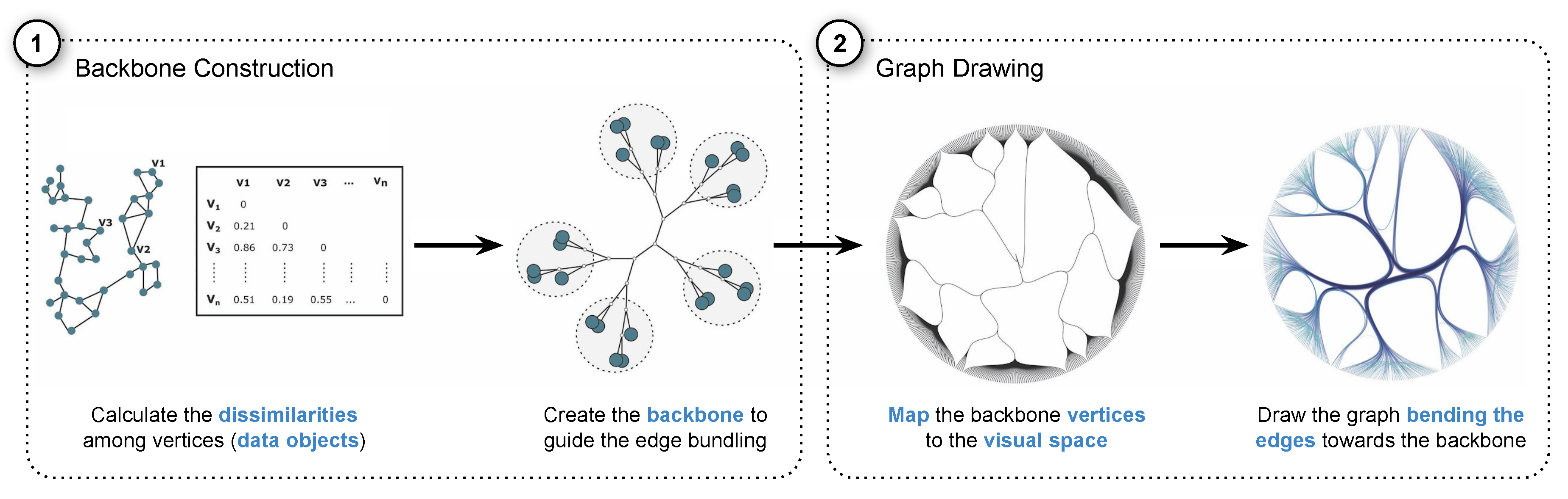
SDEB accomplishes this through a two-step process. First, a tree-like structure is created defining a backbone to guide the bundling process containing intermediate vertices that connect the data vertices or data objects based on their similarity. In the second step, the backbone vertices (data and intermediate) are mapped to the two-dimensional visual space, and edges are bent following the paths defined by the backbone. Figure 1 outlines this process. In the next sections, we detail these two steps and explain our design choices.
3.1. Backbone Construction
The backbone is a tree-like structure composed of intermediate vertices linking the data vertices V of G. As discussed, its primary function is to serve as a guide to bend the edges to generate the bundles. In the backbone, every pair of data vertices is linked through a sequence of vertices defining a path that pass through different intermediate vertices. When drawing the bundled graph, each edge that connects and is then curved towards the path . In the backbone various paths share intermediate vertices, so if i is carefully constructed, the bundling process results in groups of curved edges based on the data objects similarity.
The backbone is a crucial piece of our approach and must obey different design principles: (1) it should define paths between all pairs of data vertices, precisely connecting them according to their similarities, that is, paths between similar data vertices should contain less intermediate vertices than paths between dissimilar data vertices; (2) a unique path should connect any two data vertices, and; (3) a path between two data vertices should not pass through any other data vertex.
The first and second principles are straightforward. Since the backbone is used to attract edges for bundling, it must have paths connecting all pairs of data vertices as there could be edges between any pair of data vertices. Also, the path connecting two data vertices should be unique to avoid ambiguity problems during bending. the third principle is more involving. Suppose an edge connects the vertices and , but that neither nor are connected to another vertex . Since the backbone is used to attract towards the path , if , the edge will be bent towards , giving the wrong impression that and/or are connected to , potentially resulting in misleading visual representations.
Amongst the candidate techniques for constructing the backbone, the minimum spanning tree [31] built on top of a nearest-neighbor graph is discarded since it violates the principle (3). We also discard hierarchical clustering techniques, such as the Unweighted-pair Group Method with Arithmetic Means (UPGMA) [32], since it is sensitive to certain distance distributions [33], and prone to produce unbalanced structures violating (1). Although Neighbor Joining (NJ) [34] algorithm for phylogenetic tree construction obeys all the design principles, its applicability is limited to graphs with few nodes due to its high computational cost (). Based on these considerations, we have developed Similarity Tree (STree), an algorithm for the construction of the backbone that addresses all the design principles while presenting a lower computational cost (). STree is next described.
Similarity Tree (STree)
As already explained, the backbone is a tree-like structure where the intermediate vertices are internal vertices, and the data vertices V are leaves. Also, to satisfy our primary goal of bundling according to the similarities amongst vertex groups, the length of the path between any two vertices must be proportional to . To create such a backbone, we adapt the bisecting k-means strategy [35] algorithm to construct a binary tree where the data vertices are iteratively split into clusters and sub-clusters, defining a similarity hierarchy. It starts with one cluster C containing all data objects, representing the backbone root. Then, C is split into two new (sub)clusters and , so that each contains the most similar data objects between themselves, minimizing
where and represents the centroids of and , respectively, calculated as
where represents the number of objects in .
Once and are computed, they are attached as left and right children of C, and the same process is recursively applied to them. This splitting process continues until singleton clusters, clusters containing only one data object, are created. The backbone tree structure is then extracted from this hierarchy of (sub)clusters considering each non-singleton cluster centroid an intermediate vertex linked to its parent intermediate vertex or (sub)cluster centroid. the singleton clusters centroids are the leaves of this structure and represent the data vertices.
The process for the backbone construction is outlined on Algorithm 1. It receives a data set D and though a recursive linking and splitting process, where more compact clusters are generate after each split, returns a tree T that obeys the previously mentioned design principles. In this algorithm, the function Centroid returns the centroid of C (see Equation (2)), and the function Pivots first calculates the centroid of C then finds the further data object from as the first pivot and the further object from as the second pivot .
| Algorithm 1 Similarity Tree (STree) algorithm. | |
| functionSimilarityTree(D) | |
| ▹ assign all data objects/vertices to the first cluster C | |
| Centroid(C) | ▹ create a tree T and set its root as the centroid of C (first intermediate node) |
| SimilarityTreeRec(C, ) | ▹ generate the complete tree |
| return T | |
| end function | |
| functionSimilarityTreeRec(C, ) | |
| if then | ▹ If the input cluster C has more than one data object |
| Split(C) | ▹ split C into two clusters |
| Centroid() | ▹ set the left child of as the centroid of |
| Centroid() | ▹ set the right child of as the centroid of |
| SimilarityTreeRec(, ) | |
| SimilarityTreeRec(, ) | |
| end if | |
| end function | |
| functionSplit(C) | |
| Pivots(C) | ▹ select initial pivots for splitting |
| while MAX_ITERATIONS do | |
| ▹ Initialize the cluster | |
| ▹ Initialize the cluster | |
| for all do | |
| if then | |
| ▹ add to cluster | |
| else | |
| ▹ add to cluster | |
| end if | |
| end for | |
| Centroid() | ▹ update the pivot of |
| Centroid() | ▹ update the pivot of |
| end while | |
| return | |
| end function | |
This process creates a hierarchical structure in which in which the deeper the cluster (from the root to the leaves), the more similar the objects are. As a result, the most similar objects are closely placed on the backbone, and the path between them is reduced (design principle (1)). Also, the vertices are linked through unique paths (design principle (2)) and the path between two data vertices only contains intermediate vertices (design principle (3)).
3.2. Graph Drawing
Once the backbone is created, the next step is to map the graph onto the plane. This mapping is accomplished by defining the positions of the backbone vertices (intermediate and data vertices) on the visual space then bending the graph edges towards it. These two steps are next described.
3.2.1. Positioning the Vertices
Although different algorithms and strategies for mapping a graph onto a plane exist, most of them are computationally expensive, especially those seeking to preserve distance relationships between vertices [4]. To address such a limitation, in our approach, instead of mapping the graph G, we map the backbone. Since the backbone is a binary tree, its mapping requires less computation. In this paper, we use two different strategies to make a better use of the available space, and to improve vertices’ distance preservation: the radial layout algorithm [36] and an adaptation of the H-tree algorithm [37].
In the radial layout, the data vertices are distributed around a circle, and the backbone’s intermediate vertices are placed on the inner concentric circles, with its root in the center. In this paper, the distribution of data vertices V on the circle follows the order imposed by the backbone. the data vertices (leaves) are placed side-by-side following a canonical post-order traversal (visiting the left sub-tree, right sub-tree, and then processing the vertex). Hence, the vertices one-dimensional mapping on the circle preserves the distance relationships encoded by the backbone up to an extent. An interesting feature of the radial layout, particularly useful for bundling, is that it focuses on edges instead of vertices’ spatial positioning. Thereby, there is more visual space to present the graph connections and reduce the visual clutter.
On the other hand, the H-tree layout is focused on vertices. In the original H-tree algorithm, the vertices are positioned through a recursive process linking nodes trough perpendicular line segments, resulting in a fractal structure with a repeating pattern that resembles the letter “H”. In this process, the root vertex, is initially placed in the center of the visual space R. R is then vertically (or horizontally) split into two regions of equal areas, and , to contain the root’s sub-trees. the root’s child nodes, and , (if they exist) are placed in the center of these two regions respectively, and are linked to through a horizontal (or vertical) line segment. the regions and are then horizontally (or vertically) split to contain the sub-trees of and , respectively, and the children of and are linked through vertical (or horizontal) line segments to them. This process continues until all vertices are drawn.
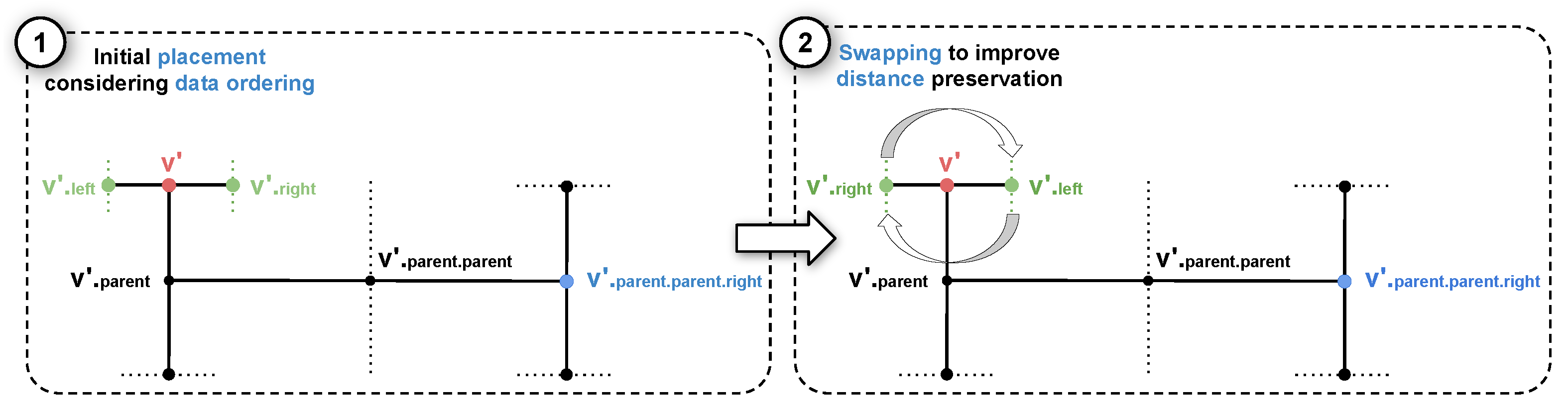
In the original H-tree algorithm, distance are not taken into consideration in the drawing process. So we modify it to preserve vertices’ distances on the produced layouts by swapping sibling vertices. the idea is outlined on Figure 2. Considering that the vertex (in red) on the sub-tree ➀ has been processed, and coordinates on the plane have been assigned to it. Before processing its children sub-trees, and , a test is performed to check if swapping them improves the distance preservation regarding the sibling of its parent (in blue). Recall that and represent centroids of two (sub)clusters of data vertices, and that represents a (super)cluster encompassing other similar (sub)clusters. Thereby, swapping with (in green) to place the most similar vertex, and therefore all its descendant vertices, closer to , and therefore all its descendant vertices, when drawing the tree potentially improves the distance preservation between the clusters represented by and with respect to . The same applying to any other vertex of the backbone. In Figure 2, the sub-tree ➁ represents the resulting drawing swapping with , putting closer to in case . Since only swaps between siblings are allowed, this adaptation can lead to a better overall distance preservation without corrupting the tree topology.
Notice that this swapping strategy performs only local modifications, so it is not guaranteed that it produces the H-tree arrangement that best preserves the distance relationships on the plane. However, a global rearrangement is impracticable to be solved for large datasets. Nevertheless, due to the triangle inequality axiom of distance metrics, we expect to improve (when possible) the results of any given tree. The complete process is detailed on Algorithm 2. In this algorithm, initially the root is set to the origin of the visual space. Then, the root’s children are linked to it using horizontal (or vertical) segments placing them equidistantly from the root’s position. This process is recursively applied taking the children as roots of subtrees and alternating the segment directions perpendicularly, reducing the distance to the (sub) roots every recursion to avoid overlaps. In this process, every time the children of a (sub) root are placed, a test is performed to check if swapping their position improves distance preservation. In the algorithm, the function SwapSiblings is used to swaps sibling vertices and in this proces.
| Algorithm 2 Swapping H-tree algorithm. | |
| functionSwappingHTree(T) | |
| SwappingHTreeRec(, , ) | |
| return T | |
| end function | |
| functionSwappingHTreeRec(, , ) | |
| if then | ▹ Set the root vertex to the layout’s center |
| else | |
| if then | ▹ If it is an horizontal placement |
| if is left child then | |
| else | |
| end if | |
| else | ▹ If it is an vertical placement |
| if is left child then | |
| else | |
| end if | |
| end if | |
| Swap() | ▹ Swap the children of if it improves the layout |
| SwappingHTreeRec() | |
| SwappingHTreeRec() | |
| end if | |
| end function | |
| functionSwap() | |
| if then | ▹ If the parent of is a left child |
| if then | |
| SwapSiblings(, ) | |
| end if | |
| else | ▹ If the parent of is a right child |
| if then | |
| SwapSiblings(, ) | |
| end if | |
| end if | |
| end function | |
As mentioned before, different from the radial layout, the H-tree layout focuses on the vertices instead of on the edges. Therefore, the distances between the data objects can be better preserved. However, it is expected to generate more cluttered visual representations due to the reduced space for the edges, although we can reduce it by assigning weights to the vertices that reflect their degree on the original graph (discussed in Section 4). Also, notice that since our modified H-tree algorithm draws a tree avoiding edge crossing, this ensures that most bundled edges only intersect the vertices on their ending points, reducing ambiguity problems.
3.2.2. Edge Bending
The second task for drawing a graph is to bend the edges to create the bundles. In this process, for each edge in G we first search for the path in the backbone that connects and . Then, we bend towards considering its vertices as control points of a B-Spline curve.
We apply filtering strategies to remove control points (intermediate vertices) to improve the visual representation and curvature of the resulting bundles. To perform this, the function determines if an intermediate vertex should be used as a control point or not. The edge is then curved towards the path , in which I is the set of intermediate vertices in the path . is defined as
where is the level (considering the backbone hierarchy) of each intermediate vertex , for instance, since it is defined in the first STree algorithm iteration.
This filtering avoids bundling edges towards less significant intermediate vertices (), that is, vertices that most (or all) data vertices are connected to, for instance, the root and the vertices in its vicinity (the intermediate vertices created in the first splittings). On the other hand, intermediate vertices close to data vertices are more significant () because they aggregate few edges. Setting this boundary affects the level of clutter reduction and allows users to create multiple graph views.
After filtering the control points, the edges’ curvatures are controlled by moving the control points towards the straight lines connecting and . This process is similar to the approach presented in [11]. However, instead of utilizing a constant value to control all edges’ curvatures, values are calculated for each edge based on their path in the backbone. Given the position of the vertex , its transformed position is calculated as
where, and are the positions of the edge ending points, k is the index of in , and is a function that controls the bending defined as
where, is the minimum size for edges to be bundled, is the strength of curvature for bundled edges and is the strength of curvature for unbundled edges. In addition, is the original edge length (Euclidean distance in the visual space). Usually, is set with a value close to 1, while is set with a value close to 0. Basically, this manipulation creates a function with a hard-step that works as an activation function. This function considers the size of each edge and determines if it should be placed in a bundle or drawn as a straight line. There is no definition for the best values of and , indeed they are parameters that users can change interactively.
4. Results and Evaluation
In this section, we evaluate Similarity-driven Edge Bundling (SDEB) three main components: the STree algorithm to create the backbone, the swapping version of the H-Tree layout algorithm to preserve distance information, and the entire edge bundling process. We quantitatively compare the STree and swapping HTree strategies with their existing counterparts, and assess the entire bundling method qualitatively comparing with other bundling techniques.
4.1. Quantitative Analysis
In the quantitative analysis, four distinct datasets with different distance distribution of data objects are used. The wdbc is a breast cancer dataset obtained from digitized images of breast masses [38]. In this dataset, most data objects are similar between themselves with a few dissimilar ones. The twonorm and simplex are artificial datasets generated using the mlbench package [39]. The first one is composed of multidimensional points from two Gaussian distributions with a unit covariance matrix. The second one consists of m-dimensional spherical Gaussian points with a predefined standard deviation and mean at the corners of a m-dimensional simplex. There is a balanced distribution between similar and dissimilar objects in both cases, composing well-separated groups of data objects. The text dataset is a vector space model representation of scientific papers from four distinct areas [40]. Most data objects are dissimilar with few similar objects in this dataset, a feature normally found on high-dimensional sparse spaces.
4.1.1. Backbone Evaluation
To evaluate the quality of trees produces by the Similarity Tree (STree) algorithm (see Section 3.1), we compare it with the Neighbour Joining (NJ) [34] and the UPGMA hierarchical clustering [32] since both present the same goal of distance preservation.
In the first test, we assess the neighborhood preservation of the original space conveyed by the three different techniques. In other words, objects belonging to the same neighborhood should be closely linked in the tree. The neighborhood preservation of a data object is calculated as follows: first we compute the k-nearest neighbours of , resulting on a list . Then, for each element we compute how many tree nodes are necessary to traverse from the node representing to the node representing (the length of the path) using the selected technique and call it . The preservation of is the median of , in which lower values indicate higher (local) distance preservation. We are evaluating the design principle (see Section 3.1), that is, well-constructed trees (backbone) are the ones that closely link the most similar objects, and consequently, result in a layout where similar objects are positioned close to each other.
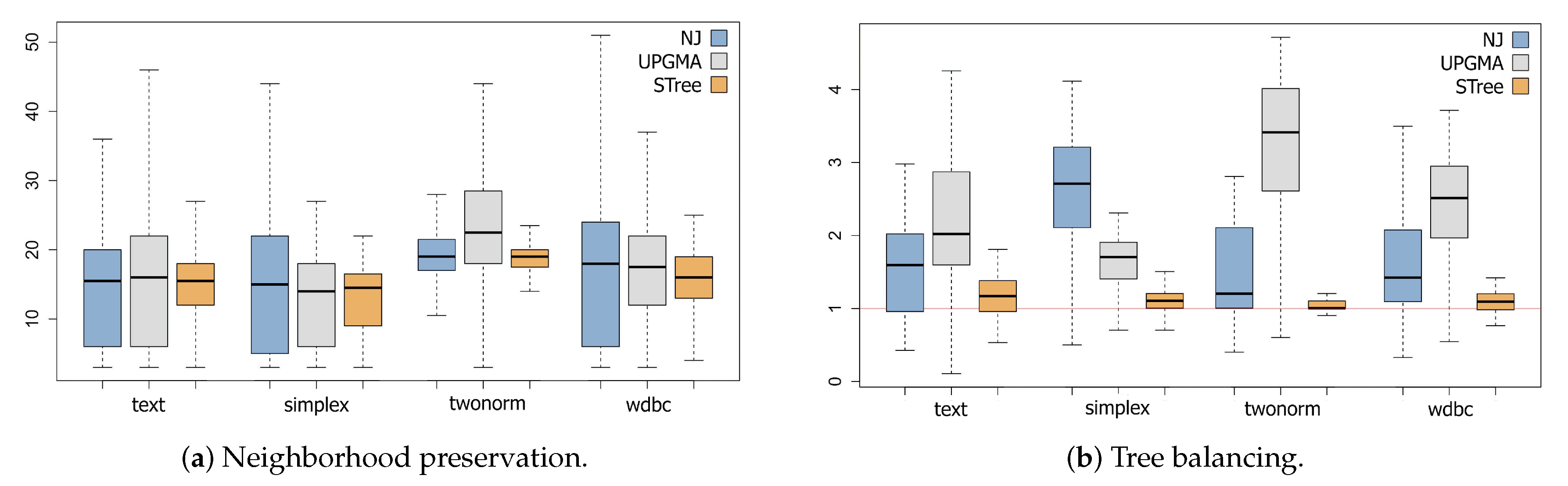
Figure 3a presents boxplots summarizing the neighborhood preservation comparing three techniques considering each dataset. The blue, gray, and orange boxplots represent the results obtained using the NJ, UPGMA, and STree techniques, respectively. These boxplots were obtained by varying the neighborhood size in the range , and computing for each data object. On average, the neighborhood preservation attained by the STree is similar or better compared to what is produced by other more computationally expensive techniques (NJ is , UPGMA is , and the STree is ). Also, the deviation from the average is smaller, indicating that the structure produced by the STree is more stable and reliable since the degree of neighborhood preservation is uniformly distributed over the entire tree.
Another critical aspect of a good backbone is how balanced the tree structure is. Less intermediate vertices (on average) need to be traversed to go from one leaf (data vertex) to any other leaf on balanced trees. Therefore, resulting in visual representations containing less distorted edges since less bending is introduced (see Section 3.2.2). For the radial layout, this results in edges with uniform curvatures, avoiding long distorted edges. There is also a more consistent use of the available visual space, especially for the H-tree layout. The vertices are more uniformly distributed over the visual space, reducing the visual clutter. Figure 3b presents the result comparing the balance of STree with the other techniques considering each data set. The blue, gray, and orange boxplots represent the NJ, UPGMA, and STree techniques. To compute the balance, for each data vertex (leaf), we calculate its depth from the root and divide by , where n accounts for the number of vertices. A tree’s balance is then the average of the balance of its data vertices (leaves). The red line represents the results of a perfectly balanced tree (equals one). On average, the STree yields considerably more balanced trees, with results very close to the red line while the other techniques deviate from it.
4.1.2. Swapping Evaluation
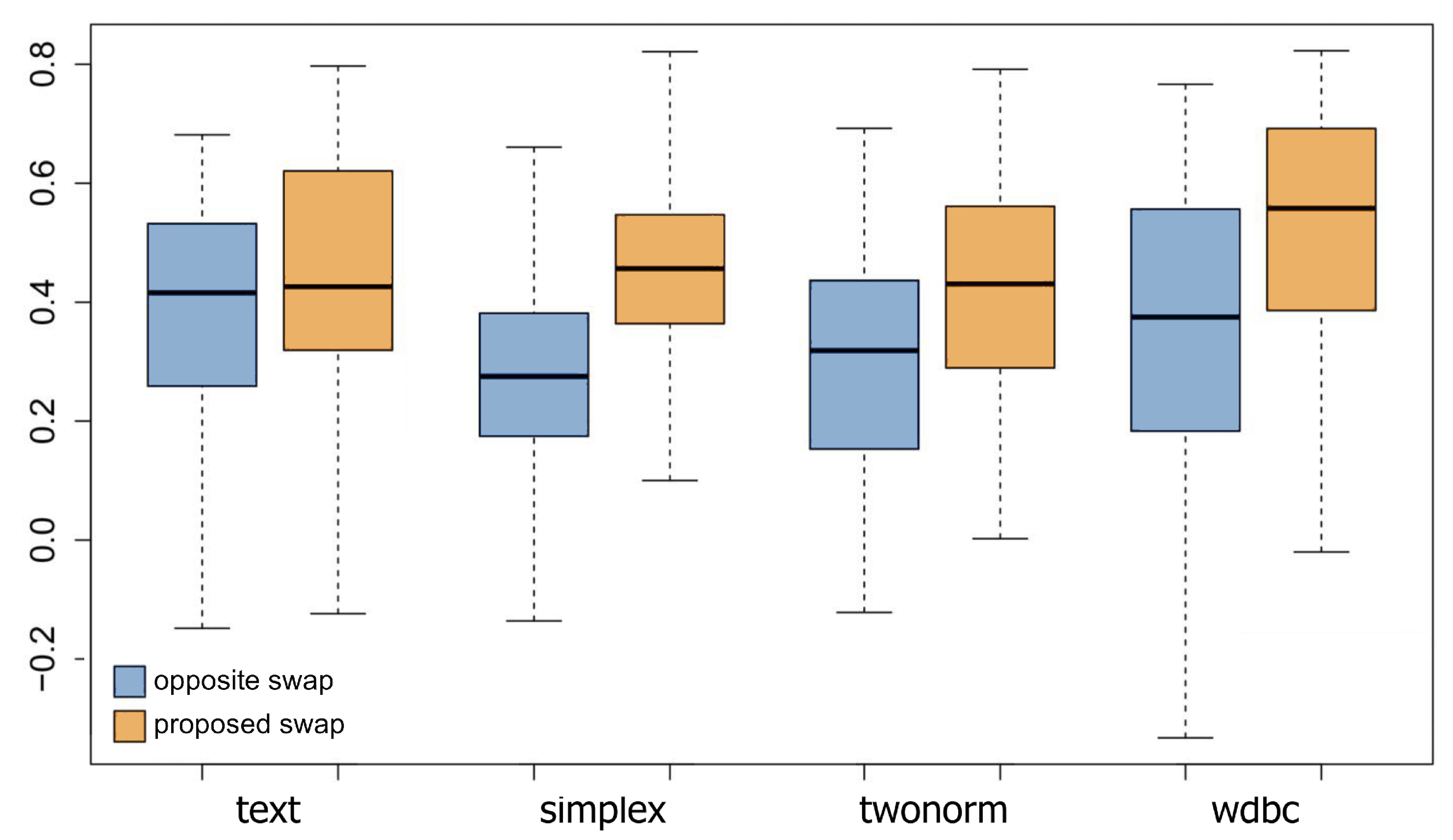
The H-tree swap strategy effectiveness to improve the produced layout’s distance preservation is evaluated in this section. By distance preservation, we refer to which degree the pairwise distance between data objects is preserved on the visual space considering the vertices’ positions. This type of evaluation’s most common approach is a metric stress function, such as the Kruskal stress [41]. However, such a metric evaluation does not apply to our case since the tree’s topology is utilized for positioning them, which results in the edges’ lengths not to be directly proportional to the distances. Therefore, we opt to use a non-metric evaluation based on the distances’ ranking. To compute the distance preservation of a data object , a rank comparing the data objects in D with is calculated in which 1 is assigned to the most similar and n to the most dissimilar data object, where n represents the number of data objects. For the corresponding vertex , we calculate another rank comparing its position on the plane to the positions of the other data vertices (leaves) on the plane, assigning 1 to the closest vertex and n to the most distanced one. The distance preservation is then computed comparing both ranks using the Spearman rank-order correlation coefficient [42], given by
varies in the range of , with large values indicating higher rank-order preservation or, in our case, distance preservation.
The boxplots in Figure 4 summarize the results of our swapping strategy for each dataset. This figure compares our proposed swap with the opposite swap since it would produce the worst results in theory. The blue boxplots represent the opposite swaps, and the orange boxplots represent the proposed swaps. For all datasets, the proposed swap’s average distance preservation is higher than the opposite swap. Only for the text dataset this improvement is not apparent. This is an expected outcome since, for this dataset, the distance distribution is highly skewed without a clear separation of objects that can be used for ranking. Such distance distribution is usually observed in high-dimensional sparse spaces, like bag-of-words of document collections. It is known that distance metrics are ill-defined in such spaces.
4.2. Qualitative Analysis
A few metrics have been proposed to compare and evaluate edge bundling layouts. For example, Gansner et al. [15] calculated the amount of ink saved to measure the clutter reduction but did not address the graph readability. Another metric is the bundling stress proposed by Nguyen et al. [43]. This metric aims to measure the difference between edges’ compatibilities and their distance in the bundling layout based on Kruskal’s stress. Although this metric seems promising for our scenario, we could not determine a reliable way to compute the edges’ compatibility. Therefore, we qualitatively compared our technique against others since, in general, there is no accepted way to measure the quality of a bundling [8]. We chose one method from each group of techniques presented in Section 2 for the comparisons. From the group of image-based techniques, we select CUBu [27]. The techniques FDEB [10] and MINGLE [15] were selected to represent the force-based and the geometry-based techniques, respectively. We generated CUBu layouts using the authors’ source code, while for MINGLE (https://github.com/philogb/mingle) and FDEB (https://github.com/upphiminn/d3.ForceBundle) we use open source libraries.
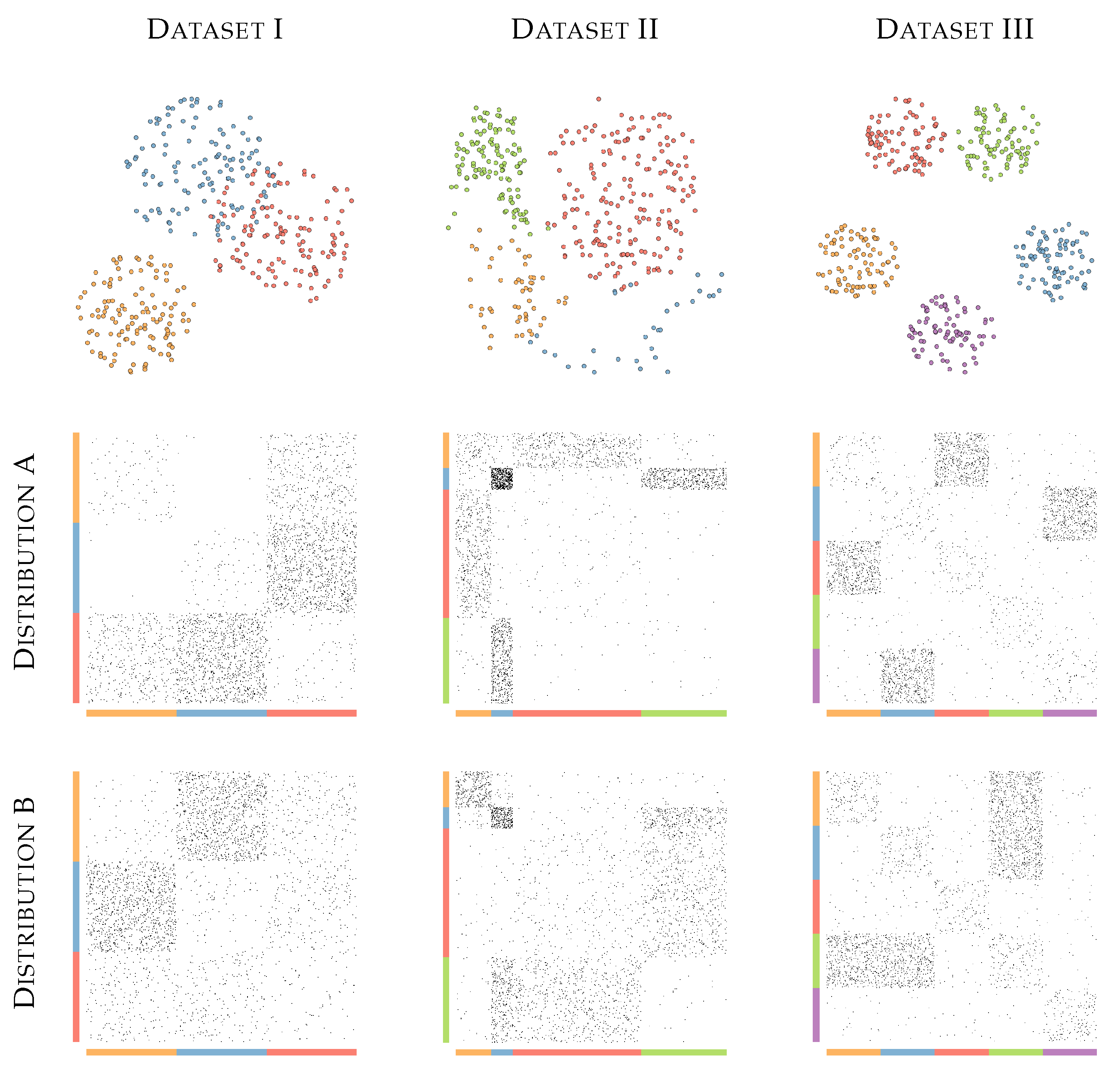
For the evaluation, we artificially generate graphs combining distinct distance relationships among data objects (vertices) and edges distributions to cover different scenarios and better control the experiments. We combine three sets of vertices with two different sets of edges distributions. Dataset I has 360 data objects in 3 groups with equal numbers of objects. Objects of two groups have some overlap, while objects of the third are well-separated. Dataset II has 380 data objects separated in 4 groups with varying sizes, containing 50, 30, 180, and 120 objects. These 4 groups are separated, but the borders between them are not well-defined. Finally, Dataset III has five well-separated groups with 80 data objects in each. Scatterplots of these datasets (they are 2D points) are presented in the first row of Figure 5. We define two different edges distributions for each data set, Distribution A and Distribution B, representing different patterns of edges connecting vertices of different groups. Figure 5 presents the resulting 6 graphs using adjacency matrix visualizations. All graphs have 1600 edges.
4.2.1. Bundling Evaluation
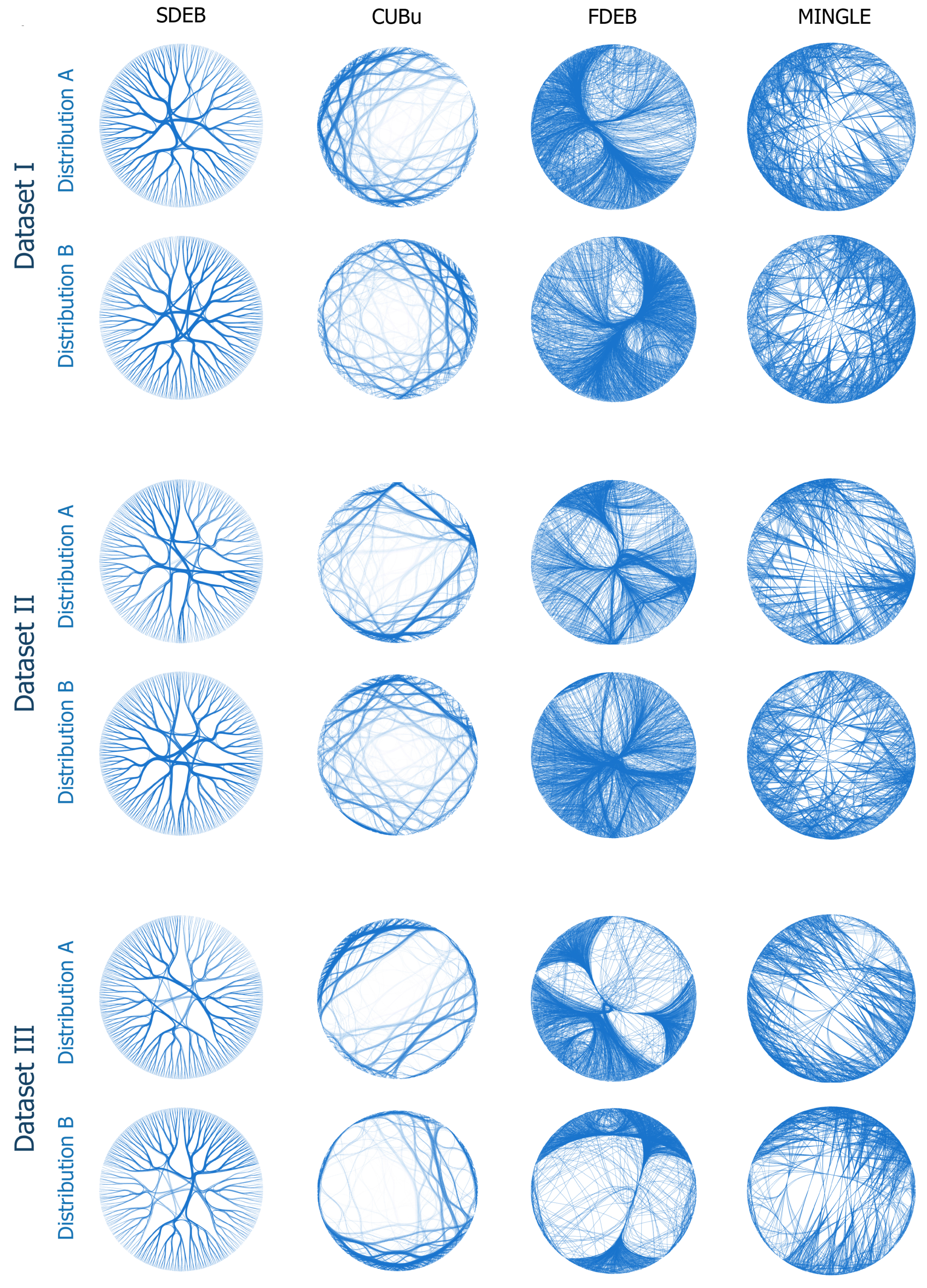
We compare the Similarity-driven Edge Bundling (SDEB) technique with CUBu, FDEB, and MINGLE considering both the radial and the swapped H-Tree layouts. Since these techniques rely on vertices’ positioning, we use the same vertices placement given by our backbone for all layouts. For all techniques, we determined the best possible parameters for such input graphs. For the SDEB, we set a filter of intermediate vertices to drop the first two levels of the STree (more details in Section 4.2.2). The comparisons considering the radial layout are presented in Figure 6.
For all graphs, we noticed that FDEB and MINGLE fail to present well-defined bundles. The worst results were presented by FDEB, which could not create any meaningful bundle, resulting in an entirely disorganized layout. MINGLE creates bundles with a few edges. However, the layout is heavily cluttered in the border of the visualization. Moreover, FDEB and MINGLE present several “outlier” edges, i.e., edges that are not grouped into any bundle. CUBu presents less cluttered layouts. The expected dense connections between groups are recognizable, as shown in the adjacency matrix presented in Figure 5. However, this technique generates bundles leaving the center of the visualization empty and the border crowded with too much information.
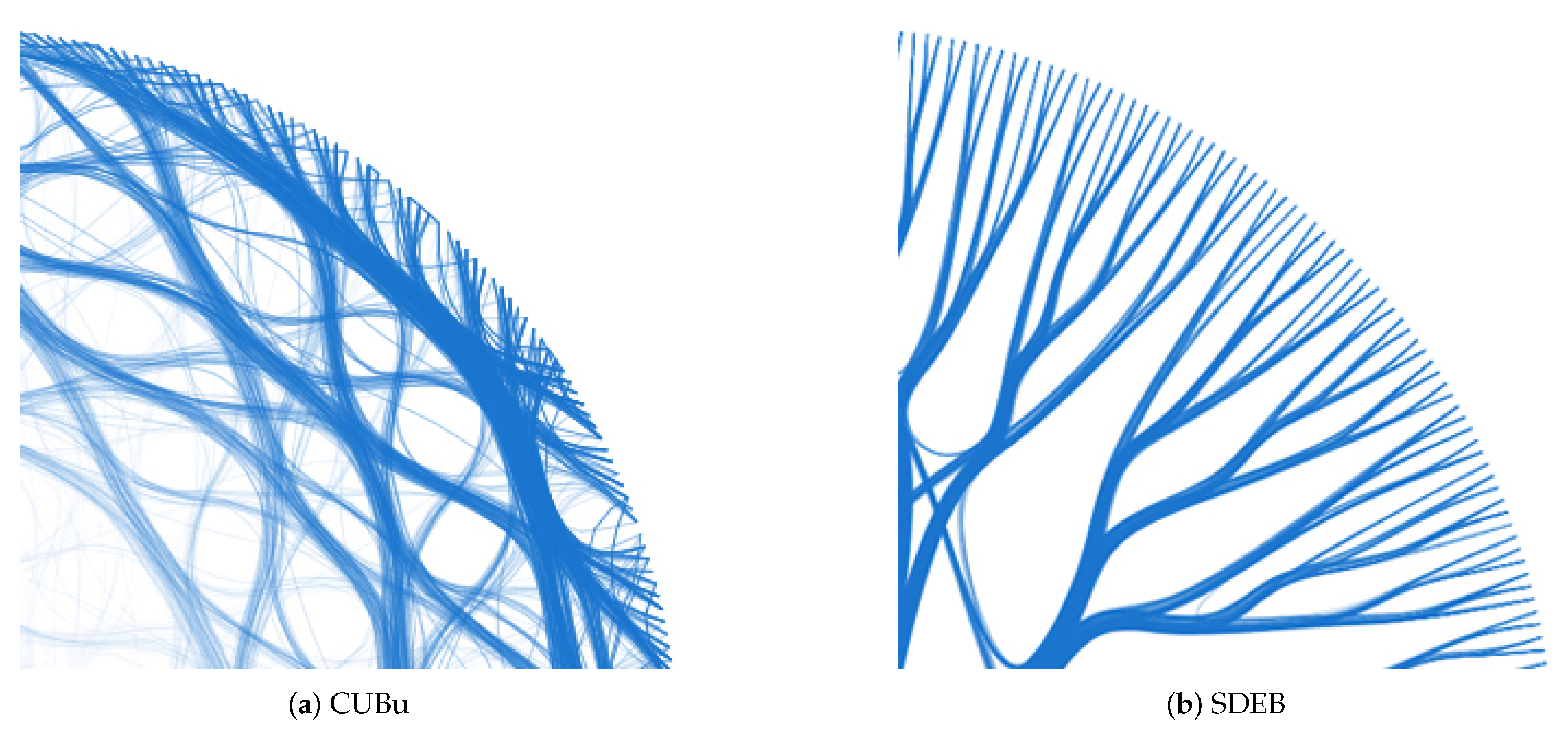
Different from CUBu, SDEB does not agglomerate the edges around the border of the visualization. Instead, our technique follows the backbone, which distributes the bundles making better use of the visual space. Most crossings in the SDEB layout happen in different directions, reducing ambiguities resulted from edges crossings. Figure 7 shows in detail the differences between CUBu and SDEB. CUBu bundles all edges close to their source/target vertices, resulting in misleading bundles. SDEB draws edges following a direction perpendicular to the radial layout’s tangent, with the bundling happening at different levels. Besides, CUBu seems to mix several bundles in a way that disregards bundles’ meaning. On the contrary, SDEB defines bundles in which it is possible to identify the groups of vertices represented in each bundling.
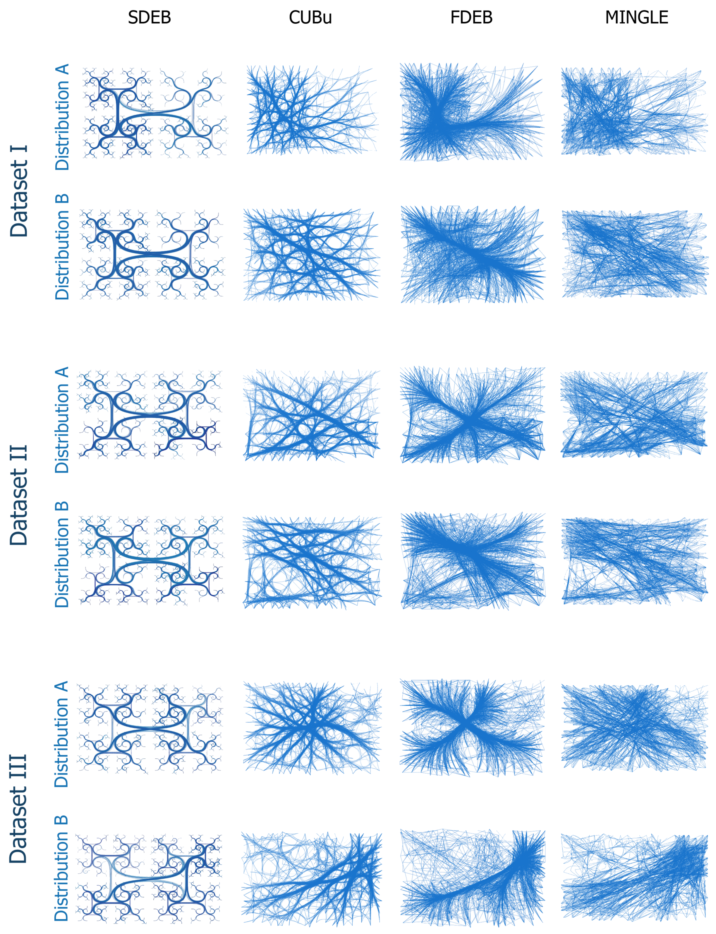
Figure 8 presents the resulting bundling comparing the same techniques but using the swapped H-Tree layout to position the vertices. As explained in Section 3.2.1, the H-tree layout focuses on the vertices, spreading them through the visual space. Even though the techniques share the same vertices position, the difference in bundling readability is evident. This happens because CUBu, FDEB, and MINGLE generate the bundles only considering spatially-similar edges trajectories, while our technique follows the backbone, which is mapped to the plane using the H-Tree technique. Our approach takes advantage of the H-Tree layout to produce more compact bundles and a less cluttered representation than any other technique. Also, vertices placed in the center of the visualization are easier identified. Although there is some overlapping of edges over vertices, this occurs less often than in the other techniques, in which the bundles completely hide centralized vertices. However, the resulting bundles repeat the pattern existent in the H-Tree layout’s fractal structure, making the edges patterns harder to be identified and less visually pleasant. Despite that, we can recognize the edges patterns by analyzing bundles’ density.
These comparisons show that all the selected state-of-the-art techniques could produce edge bundling layouts that highlight significant patterns. FDEB and MINGLE produce better results when the vertices are spread over the visual space (H-Tree layout) but tend to fail to produce meaningful results for the radial layout, resulting in heavily cluttered representations. CUBu and SDEB present a better clutter-reduction, but CUBu concentrates the bundling close to the source/target edges, resulting in misleading bundlings. SDEB produces better layouts reducing ambiguities and creating more compact bundles.
4.2.2. Bundling Enhancements
In this section, we report the results of the two enhancements designed to give the user a set of options to transform the bundling visualization. These transformations are the Adaptive-, and the intermediate vertices filtering.
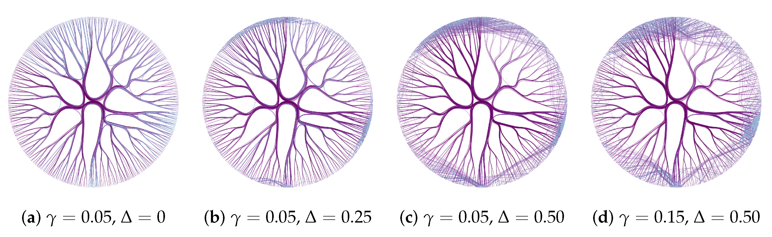
The Adaptive- enables the individual tension control of each edge. In our method, the tension, that is, the strength with which edges are attracted to the backbone is defined by three parameters: , , and (see Section 3.2.2). defines the minimum size of an edge to be bundled, is the tension for bundled edges, and is the tension for the unbundled ones. Figure 9 shows different examples varying these parameters for the same input graph. By properly setting up and different visualizations can be produced, revealing hidden local information. When (Figure 9a), short edges are hardly identified since they are mixed with long ones. When we increase the value of (Figure 9b,c), short edges are separated from the bundles, showing concealed information, such as the groups of similar vertices with more connections. However, the unbundled edges can add noise into the layouts (Figure 9d), and high values of and might make the visualization worse.
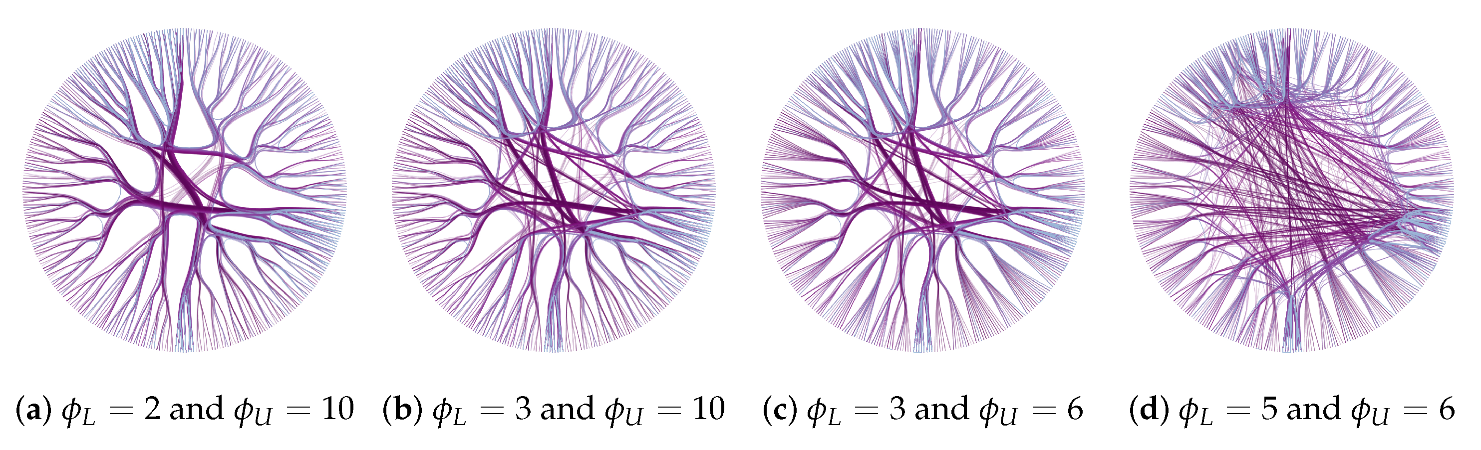
The second enhancement is the intermediate vertices filtering. In this modification, the user sets the interval defining the backbone hierarchy levels to be considered on the bundling process, so that the edges are bent only using the intermediate vertices in the interval. Figure 10 presents four variations of intermediate vertices filtering. These examples show the effects of dropping intermediate vertices from the root and the leaves of the backbone. Removing intermediate vertices closer to the root creates direct connections between groups on deeper levels, resulting in a more detailed visualization. On the other hand, dropping intermediate vertices closer to the leaves generates bigger and more generic groups.
5. Use Cases
In this section, we present different use cases applying SDEB to real-world datasets. In these scenarios, we show how SDEB can be used to explore graphs with different levels of details, how it can be applied to represent dynamic graphs bundles, and how it can be used as a multi-scale approach.
5.1. Edge Bundling Simplification
In the first use case, we use a subset of the Visualization Publication Dataset (infovis) [44] to show how SDEB can be used to explore graphs with different levels details. This subset is composed of papers with at least five citations, resulting in 384 papers (vertices) and 1633 cross citations (edges). We calculate the similarity between papers using a bag-of-words representation of their content (abstract, title, and authors list) and the cosine dissimilarity. Figure 11 shows the visualization using the radial layout. We set the parameters , , , and the filtering function of control points to and . Edges’ colors represent their sizes.
With these parameters, small edges are less bent towards the backbone, and interesting patterns emerge, for example, the high number of short edges. This is expected since similar papers are close in the radial layout, and those papers should present similar main subjects and, therefore, the same (circular) references. However, the distribution is not regular, indicating that some papers or topics concentrate more citations among related papers, while others cite the same papers less frequently. Another interpretation is that, recapping that this dataset only contains papers of the IEEE Visualization conference, some topics are more self-contained in the visualization community while others have references outside the field.
In this visualization, inter-group relationships can also be observed. However, given the number of vertices and connections, it may be time-consuming to make conclusions. To alleviate this problem, the backbone hierarchical structure can be used to summarize the graph, allowing a details on-demand approach to be employed. By applying the multi-level control in certain backbone branches, the user can select groups of similar vertices and visualize them as a single vertex. In the summarized visualization, the selection hides the grouped vertices and edges and shows the group’s information. Figure 12 presents the summarization of four groups, each one identified by a different color with the content of the hidden vertices depicted by a circle pack representation with the most frequent terms contained in the grouped scientific papers. On the right side, a list of the selected papers is displayed.
5.2. Dynamic Edge Bundling Visualization
In the second use case, we show how to use SDEB on the analysis of dynamic graphs. In this example, we create the #NBABallot dataset. The #NBABallot consists of a collection of posts extracted from Twitter related to the American National Basketball (NBA) league. To compose this dataset, we selected tweets published with the hashtag #NBABallot between 19 December 2014, and 21 January 2015. This hashtag was used to vote in a player to compose one of the two teams of the 2015 NBA All-Star Game. This election selected five players for each team, the Eastern All-Stars and the Western All-Stars. During this period, more than 2 million posts (votes) were collected.
After collecting the tweets, we processed them to create our dataset. In the resulting graph, vertices represent players, and the data used to calculate the similarity among them was extracted from the official league statistics page (http://stats.nba.com/), which covers the major statistics measures of basketball matches (e.g., points, rebounds, assists, turnovers, field goal percentage, three-point percentage, blocks, and others). Edges connect players that had received votes from the same user. This graph was segmented by tweets days, which we call a voting frame. The final graph consists of a dynamic graph with 436 vertices, 11,793 distinct edges, and 34 frames. Considering the whole list of edges, we found 565,829 associations between pairs of players who received a vote from users on the same day.
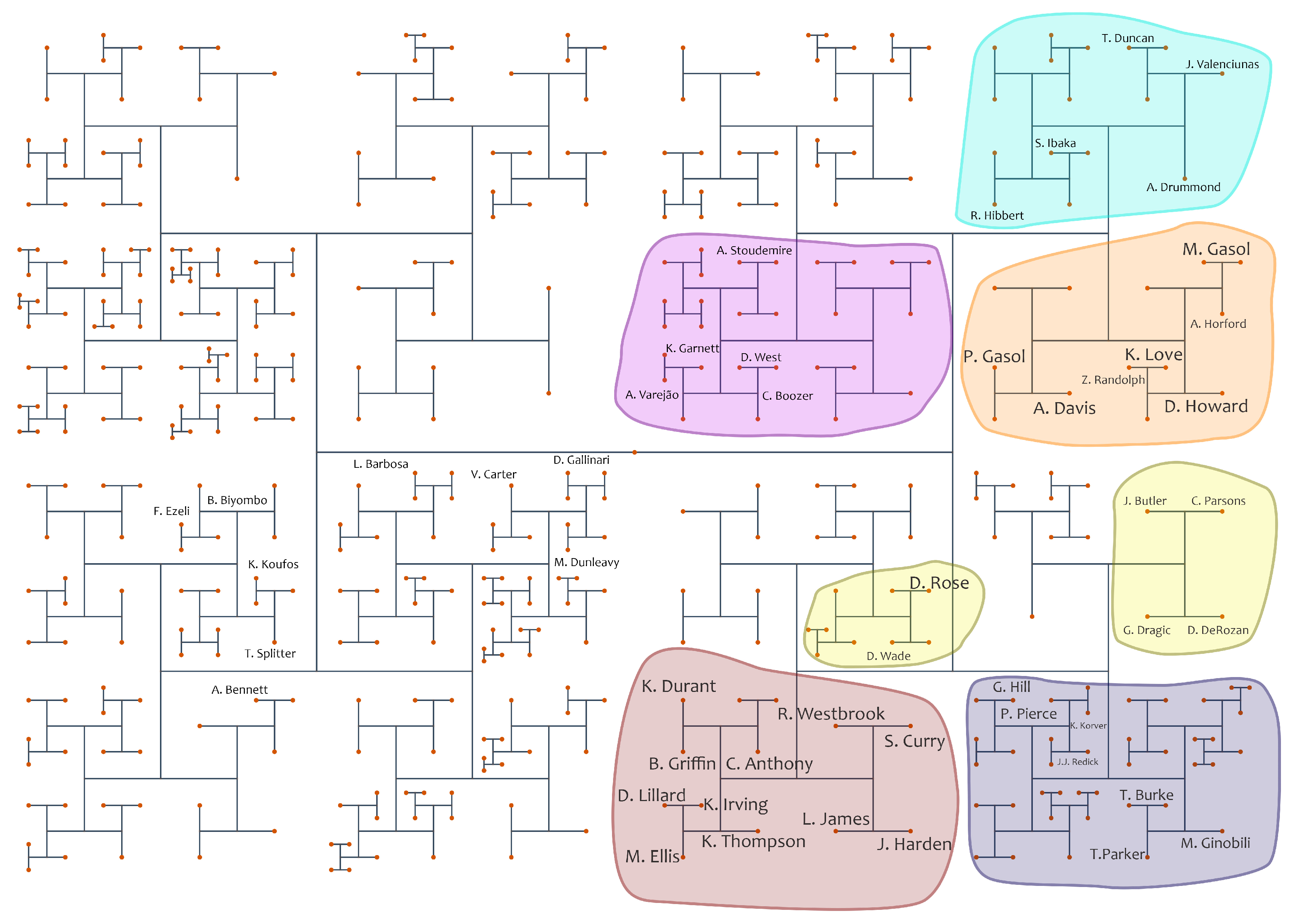
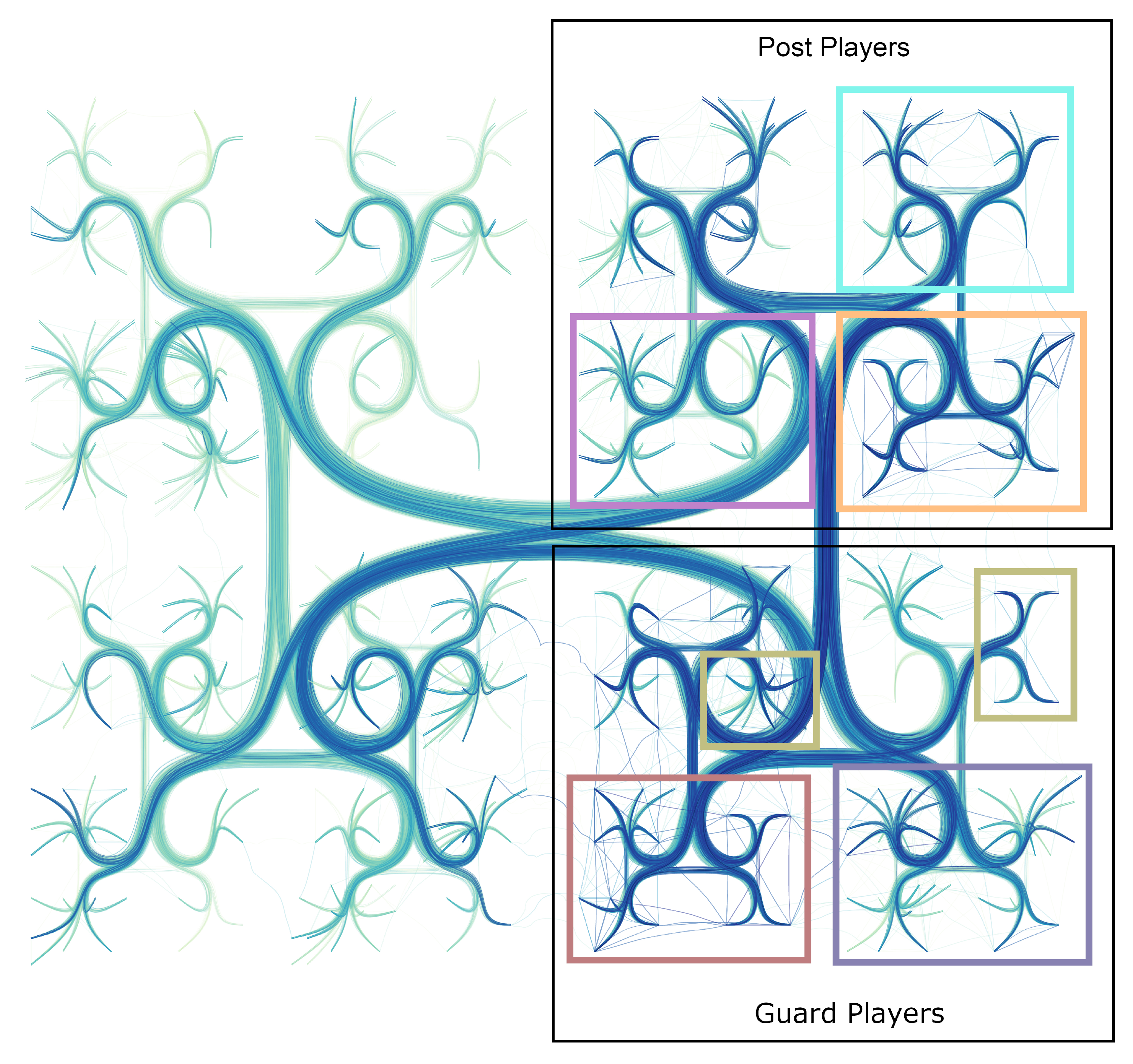
Before examining the resulting graph, we start our analysis explaining the backbone showed in Figure 13. Just to set important terms for the reader nonfamiliar with basketball, players are commonly assigned to one of five positions in the court, which are Point-guard, Small-guard, Small-forward, Power-forward, and Center. The first two positions are usually called guards, while the last two are usually called posts. Small-forward players are versatile players that may be associated with both post and guard positions, according to the team strategy. In this figure, some groups are highlighted to identify leading players. The first noticeable pattern is the first division in the backbone. It splits the players into two major groups. The first group (on the right) represents the more active players (i.e., starters or engaged bench players), while the second group (on the left) is formed by less active players (i.e., players that usually play for a few minutes). The right side concentrates the most famous athletes in the league (high on many statistics). On the contrary, players from the left side are less prominent.
After the second backbone division, it becomes harder to analyze the left side since players with a few minutes per game have inaccurate or incomplete statistics. Regarding the right side, the backbone clearly separates post players, placed at the top, and guard players, placed at the bottom. The backbone shows more similar players on deeper levels. The red group encompasses the ones considered to be the best players in the league. These players are known to have good performances in most statistics, making them the leading players of their teams. The blue group identifies players with similar abilities, but they do not have a leading role. Groups identified in yellow are similar to the red and blue groups. The players from the yellow groups are important. Still, they present good performance in only a few metrics, making it evident that it is possible to classify players according to their position on the court only using their statistics.
On the top, the players are divided into three different groups. The orange and cyan groups embrace the best post players in the league, although the cyan one covers players with less impact in their team statistics. The purple group depicts good players with a supporting role in their teams. It is noticeable that there are less post players than guard ones in the league. This is because teams usually play with only two, or even one post player, while there are three to four guards.
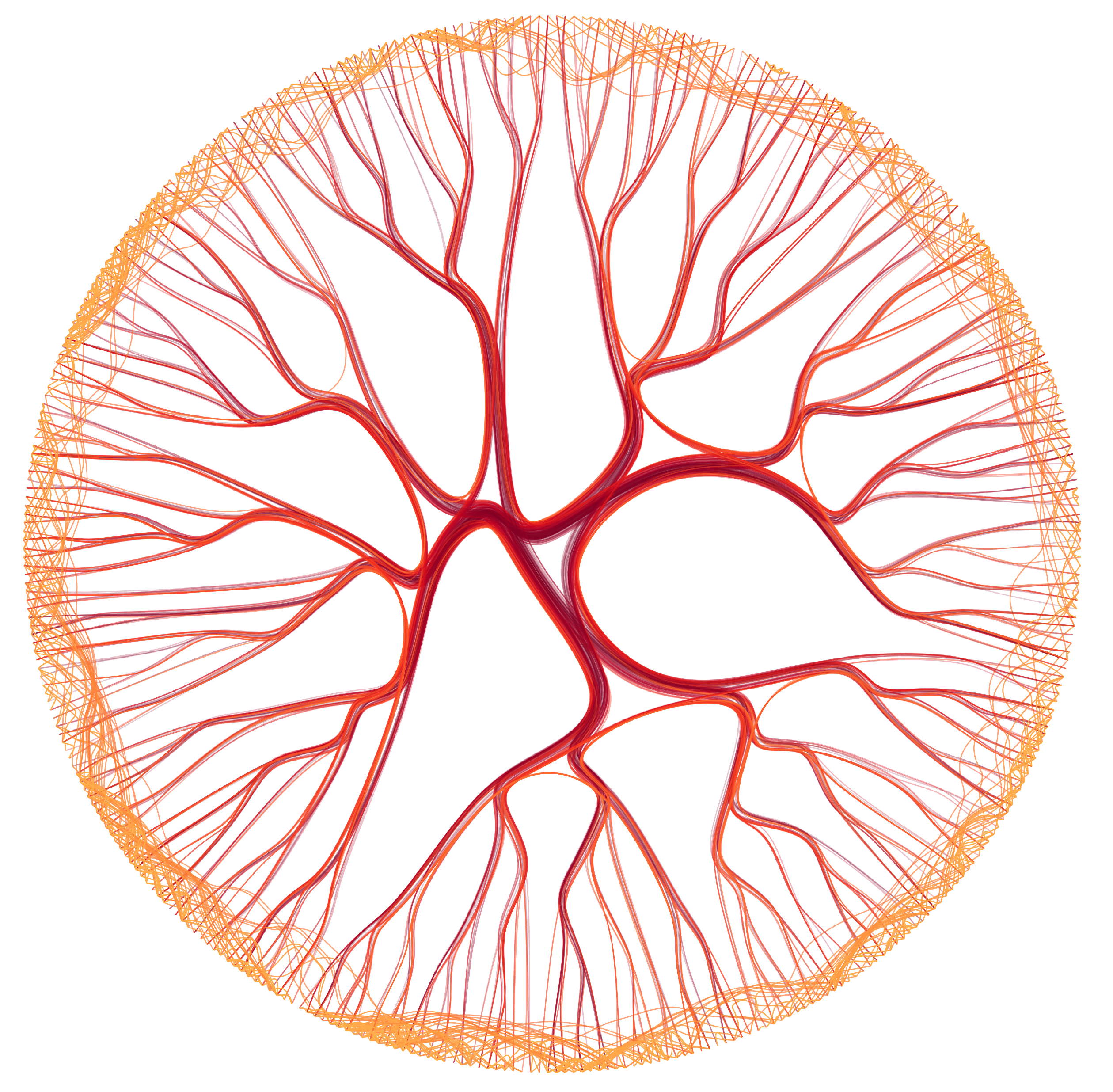
Figure 14 shows the edge bundling layout of the entire dataset (i.e., not divided in voting frames). The first recognizable aspect is the difference in the edges’ density between the left and the right sides of the graph. An expected outcome since the right side is composed of the best players (according to the statistics). Also, there are many edges connecting top-right with bottom-right players, showing a voting pattern consisting of users selecting guard and post players simultaneously, even though this is not an election requirement. Moreover, short edges, which connect similar players, are easily identified. There are many unbundled edges connecting elements inside the brown, yellow, and orange groups, while there are fewer occurrences in other areas. The visualization also shows that users usually vote in more players from those groups while selecting fewer post players. This behavior was confirmed in the election’s result, in which just three players (Anthony Davis, Pau Gasol, and Marc Gasol) out of ten were elected from the top-right side.
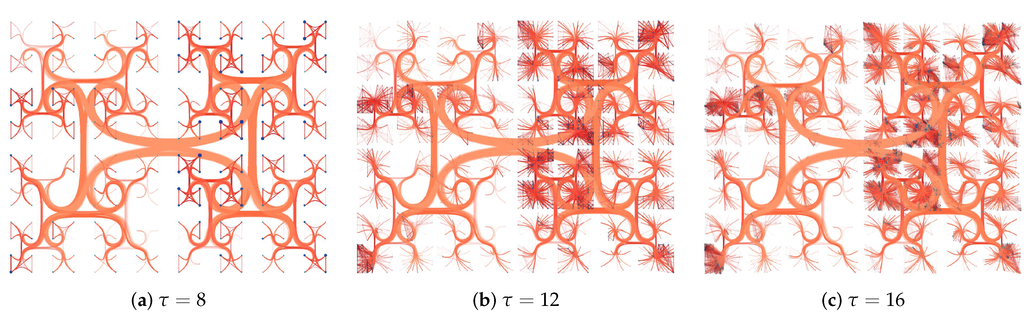
By considering different voting frames as individual graphs, it is possible to understand how the votes’ behavior changed over time. Regarding the visualization of time-varying information, there are two main metaphors to visualize such data: animation and small multiples [45]. Some studies prefer the latter since it can show different frames together [46]. In our framework, both methods can be used since the backbone is the only information used to bend edges, and it does not change over time, preserving the context. Figure 15 shows the #NBABallot graph for six selected frames using small multiples. All graphs were generated with parameters , and . The edges are colored according to the number of occurrences of paired votes. The darker the color, the more votes an edge represents.
Comparing the different frames, the dominant pattern identified in Figure 14 is also visible. However, we can observe slight modifications in each bundle’s density, such as in frames 1 and 11. Moreover, less important players (left-side) concentrates fewer edges, which provides fascinating insights. Some outlier players have several connections with the opposite side in some frames. For example, there are edges from the top-left group that only appear in frames 1, 6, and 33. A further investigation can map this behavior with events related to the election, such as game days or marketing campaigns asking for votes.
The main difference between our method and previous techniques used for dynamic graphs is stability. Techniques that compute bundles based on edges would create different bundles based on edges spatial distribution. Therefore, the same edge may be placed in different bundles when comparing different frames, resulting in potential context loss and misinterpretation. Our technique draws edges in the same bundle disregarding changes over time. Although this may be harder to analyze, it provides more reliable information.
5.3. Multi-Scale Edge Bundling Visualization
Finally, we discuss how SDEB can be used to provide insights into graphs using a multi-scale approach. In this use case, we use the Amazon Product co-purchasing Network (amazon) dataset [47]. This dataset represents more than 500,000 products from Amazon’s website and associate information, such as product category, similar products, and reviews written by clients. We consider only grocery products to focus our analysis, resulting in a graph with 8700 vertices (products) and 129,407 edges connecting products purchased together. Similarity among products is calculated using the reviews published by customers.
To create a multi-scale representation, we define a threshold limiting the maximum depth of the backbone to be used. Intermediate or data (products) vertices deeper than are filtered out from the visualization and represented by their closest visible ancestors, composing a cluster of similar vertices. Edges connecting elements inside the same cluster are also removed from the visual representation. Figure 16 shows three layouts, varying the maximum depth in which the backbone is rendered. When (Figure 16a), only 248 vertices are visible, with almost all vertices representing clusters of products. The layout with shows 2108 vertices (Figure 16b) and the layout with shows 5856 (Figure 16c), which means that only few vertices still represent clusters of products. In such cases, we also observe the congestion of edges inside more populated groups.
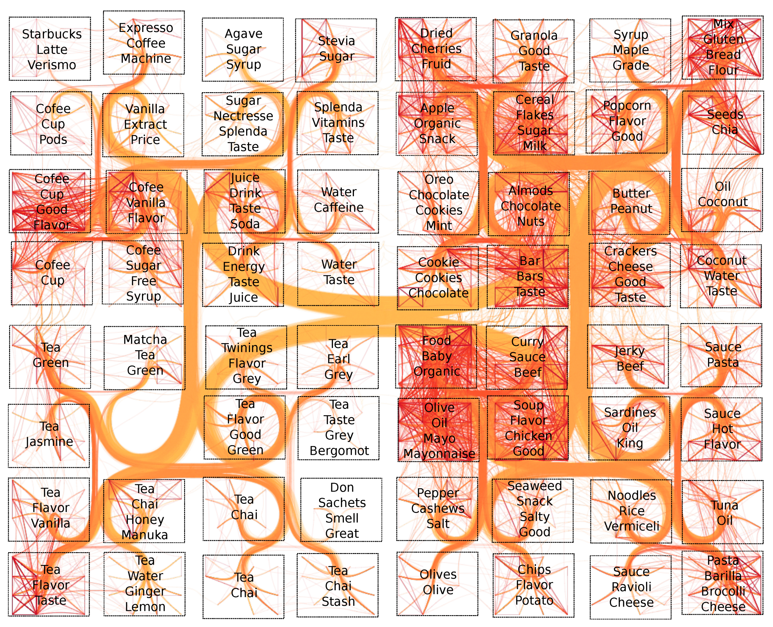
Users can change to explore the graph bundling in different levels of detail. In Figure 17 we fix and tag the 63 visible groups of products with the most common topics found in their reviews. By labeling the groups, we can see which products belong to each group. Some neighbor groups share the same topics, indicating that they were defined at a higher level and refined in the lower ones. For example, all groups in the bottom-left branch are labeled with “Tea”. Another observable behavior is that the first division segments liquid and solid groceries. The bundling layout was created using the parameters , and . This configuration also highlights dense groups, with more connections among their elements and their neighbors.
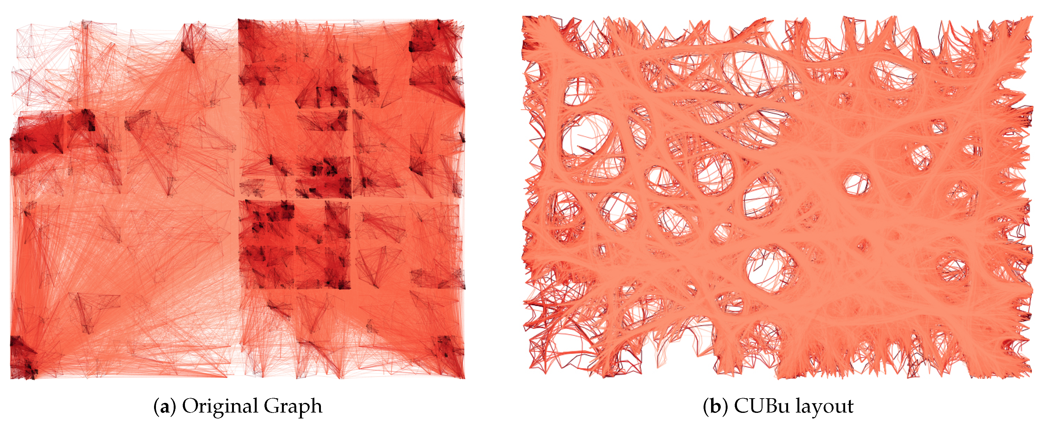
This example shows that the multi-scale layouts produced by our technique facilitate the detection of vertices and clusters. For comparison, Figure 18 presents the original graph (using straight lines to represent the edges) and the edge bundling layout produced by CUBu, the fastest technique in the state-of-the-art. Although CUBu generates the bundling in s, the layout could not organize edges into meaningful bundles, and the clutter reduction is not as significant as in the layout produced by our technique. Moreover, vertices are hidden in both layouts, especially in dense areas of edges, impacting the analysis and insights that can be derived. Our technique took around 100 s to create the backbone and 55 s to render the full graph. However, it creates a less cluttered layout where groups of products and their connections are clear.
6. Discussions and Limitations
As formalized at the beginning of Section 3, SDEB assumes that each graph node represents data objects described through numerical values. That is, the vertices represent objects embedded in a vector space. One reason is related to the very own technique’s nature, which is to guide the bundling using data information, in our case, distances between objects. The second is associated with the procedure we develop to create the backbone (Section 3.1). In this procedure, the function Centroid returns the mean of a group of data objects, and this assumes objects embedded into a (multidimensional) vector space. This limitation can be addressed using the medoid of a group of objects, the object whose average dissimilarity to all the group objects is minimal, instead of its centroid. This opens some interesting possibilities. For instance, the adjacency (edges) information could be used to compute the similarity between vertices (see [3]), resulting in bundles with a different semantical meaning.
A second limitation of our technique is the assumption that the vertices’ position preserves distance relationships (of the data objects) and is guided by the backbone. So for graphs in which the vertices positions are pre-defined, for instance, geographical location, SDEB cannot be employed. We tried to use the defined vertices positions to calculate the distances when creating the backbone to address such a limitation. However, the results were unsatisfactory (too many crossings between backbone paths), and using positions to generate the backbone instead of data information violates our design principles and the primary goal of bundling edges according to the semantic defined by data objects/vertices.
In this paper, the produced layouts were informally evaluated during their design phase using a think-a-loud process, where participants explain what they are seeing while exploring different layouts. The results were encouraging, especially for the more common circular representations, and for the H-Tree, up to a certain extent. However, these informal tests cannot be considered evidence of the proposed approach or edge bundling layouts efficacy. Despite that, they resulted in one interesting observation. The H-Tree symmetrical layouts are not as visually pleasing as the circular layouts, although this does not influence the overview interpretation of a graph. One potential solution could be running a force-directed algorithm using the swap H-Tree as the initial layout, reducing the fractal appearance but incurring possible overlaps. All in all, user evaluation is still a bottleneck, not only for our approach but also, to the best of our knowledge, to the entire field of edge bundling techniques. And a complete evaluation of bundling efficacy remains as future work and a challenge.
Although SDEB is slower than the state-of-the-art, it does not demand any special hardware to be executed, such as GPUs, being very simple to implement and execute. Also, SDEB offers a data-driven multilevel interpretation of bundling layouts, something not provided by the fastest techniques. If this is more important for a given analytical scenario, the drop in running time can be acceptable. However, if speed is mandatory, SDEB is not the best choice. Notice that our implementation is a mix of java and javascript codes, and the running times can be dramatically decreased using a GPU-based implementation. Also, observe that we have two phases in our approach (Figure 1) and the Graph Drawing phase, where user interaction happens (changing and parameters), is independent of the Backbone Construction. Therefore, for a visual analytics exploratory process, the Backbone Construction phase can be viewed as pre-processing since it is not parametric, and the Graph Drawing is much faster to execute, making the user interaction experience virtually real-time. However, these are implementation details, and running time is not the focus of our solution.
Finally, in terms of computational complexity, we can split the analysis into Backbone Construction and Graph Drawing phases. The former phase’s complexity is the basically the STree algorithm complexity (see Section 3.1). The latter’s phase complexity involves placing the backbone into the plane, finding the edges’ paths, and drawing the graph. Given that the Split function is (see Algorithm 1), where n is the number of data vertices/objects, and that it results in even splittings (which is usually the case as can be observed in Figure 3b), the overall complexity of the STree algorithm is . Using a bottom-up approach to find the shortest path between two data vertices (backbone leaves) is for a balanced tree, so, for a set of e edges, finding all shortest paths is . Using the circular layout or the swapping H-Tree algorithm (see Algorithm 2) to position the backbone is , and drawing the splines is . Therefore the overall complexity is , that is, where k is the largest between n and e.
7. Conclusions
This paper presents Similarity-Driven Edge Bundling (SDEB), a novel edge bundling technique that produces enriched semantic layouts bending edges obeying similarities relationships present on graphs (data sets). Although SDEB cannot be used when vertices have a defined position, such as geographic information, the backbone strategy allows other interesting applications. One example is the dynamic graph visualization, producing more stable bundles over subsequent time frames. Another is the multilevel exploration, enabling users to investigate bundles on different levels of details, from major connection patterns to more refined views of small groups of edges. This is the first time, to the best of our knowledge, an edge bundling technique fully supports multilevel exploration, an important feature when handling large or dense datasets.
Author Contributions
Conceptualization, F.S. and F.V.P.; data curation, F.S.; investigation, F.S., R.R.O.d.S., and G.D.C.; methodology, F.S. and F.V.P.; supervision, F.V.P.; validation, F.V.P.; visualization, F.S.; writing-original draft, F.S. and F.V.P.; writing-review & editing, E.E. and F.V.P. All authors have read and agreed to the published version of the manuscript.
Funding
This research was funded by the São Paulo Research Foundation (FAPESP-Brazil) (#2014/18665-1 and #2011/22749-8), the Coordination for the Improvement of Higher Education Personnel (Capes-Brazil) and the National Council for Scientific and Technological Development (CNPq-Brazil). We also acknowledge the support of the Natural Sciences and Engineering Research Council of Canada (NSERC).
Acknowledgments
We would like to thank all the reviewers for the valuable comments and suggestions.
Conflicts of Interest
The authors declare no conflict of interest.
References
- Iragne, F.; Nikolski, M.; Mathieu, B.; Auber, D.; Sherman, D. ProViz: Protein interaction visualization and exploration. Bioinformatics 2004, 21, 272–274. [Google Scholar] [CrossRef] [PubMed] [Green Version]
- Martin, A.; Ochagavia, M.; Rabasa, L.; Miranda, J.; Fernández-de Cossio, J.; Bringas, R. BisoGenet: A new tool for gene network building, visualization and analysis. BMC Bioinform. 2010, 11, 91. [Google Scholar] [CrossRef] [PubMed] [Green Version]
- Martins, R.; de Faria Andery, G.; Heberle, H.; Paulovich, F.; Lopes, A.A.; Pedrini, H.; Minghim, R. Multidimensional Projections for Visual Analysis of Social Networks. J. Comput. Sci. Technol. 2012, 27, 791–810. [Google Scholar] [CrossRef]
- Herman, I.; Melançon, G.; Marshall, M.S. Graph visualization and navigation in information visualization: A survey. Vis. Comput. Graph. IEEE Trans. 2000, 6, 24–43. [Google Scholar] [CrossRef] [Green Version]
- Von Landesberger, T.; Kuijper, A.; Schreck, T.; Kohlhammer, J.; van Wijk, J.J.; Fekete, J.D.; Fellner, D.W. Visual Analysis of Large Graphs: State-of-the-Art and Future Research Challenges; Computer Graphics Forum; Wiley Online Library: Hoboken, NJ, USA, 2011; Volume 30, pp. 1719–1749. [Google Scholar] [CrossRef]
- Ellis, G.; Dix, A. A taxonomy of clutter reduction for information visualisation. Vis. Comput. Graph. IEEE Trans. 2007, 13, 1216–1223. [Google Scholar] [CrossRef]
- Zhou, H.; Xu, P.; Yuan, X.; Qu, H. Edge bundling in information visualization. Tsinghua Sci. Technol. 2013, 18, 145–156. [Google Scholar] [CrossRef]
- Lhuillier, A.; Hurter, C.; Telea, A. State of the Art in Edge and Trail Bundling Techniques. Comput. Graph. Forum 2017, 36, 619–645. [Google Scholar] [CrossRef]
- Bach, B.; Riche, N.H.; Hurter, C.; Marriott, K.; Dwyer, T. Towards Unambiguous Edge Bundling: Investigating Confluent Drawings for Network Visualization. IEEE Trans. Vis. Comput. Graph. 2017, 23, 541–550. [Google Scholar] [CrossRef] [Green Version]
- Holten, D.; Van Wijk, J.J. Force-Directed Edge Bundling for Graph Visualization; Computer Graphics Forum; Wiley Online Library: Hoboken, NJ, USA, 2009; Volume 28, pp. 983–990. [Google Scholar] [CrossRef]
- Holten, D. Hierarchical edge bundles: Visualization of adjacency relations in hierarchical data. Vis. Comput. Graph. IEEE Trans. 2006, 12, 741–748. [Google Scholar] [CrossRef]
- Selassie, D.; Heller, B.; Heer, J. Divided edge bundling for directional network data. Vis. Comput. Graph. IEEE Trans. 2011, 17, 2354–2363. [Google Scholar] [CrossRef] [Green Version]
- Cui, W.; Zhou, H.; Qu, H.; Wong, P.C.; Li, X. Geometry-based edge clustering for graph visualization. Vis. Comput. Graph. IEEE Trans. 2008, 14, 1277–1284. [Google Scholar] [CrossRef] [PubMed]
- Lambert, A.; Bourqui, R.; Auber, D. Winding Roads: Routing Edges into Bundles; Computer Graphics Forum; Wiley Online Library: Hoboken, NJ, USA, 2010; Volume 29, pp. 853–862. [Google Scholar] [CrossRef] [Green Version]
- Gansner, E.R.; Hu, Y.; North, S.; Scheidegger, C. Multilevel agglomerative edge bundling for visualizing large graphs. In Proceedings of the 2011 IEEE Pacific Visualization Symposium (PacificVis), Hong Kong, China, 1–4 March 2011; pp. 187–194. [Google Scholar]
- Bouts, Q.W.; Speckmann, B. Clustered edge routing. In Proceedings of the 2015 IEEE Pacific Visualization Symposium (PacificVis), Hangzhou, China, 14–17 April 2015; pp. 55–62. [Google Scholar] [CrossRef] [Green Version]
- Telea, A.; Ersoy, O. Image-Based Edge Bundles: Simplified Visualization of Large Graphs; Computer Graphics Forum; Wiley Online Library: Hoboken, NJ, USA, 2010; Volume 29, pp. 843–852. [Google Scholar] [CrossRef] [Green Version]
- Ersoy, O.; Hurter, C.; Paulovich, F.V.; Cantareiro, G.; Telea, A. Skeleton-based edge bundling for graph visualization. Vis. Comput. Graph. IEEE Trans. 2011, 17, 2364–2373. [Google Scholar] [CrossRef] [PubMed] [Green Version]
- Hurter, C.; Ersoy, O.; Telea, A. Graph Bundling by Kernel Density Estimation; Computer Graphics Forum; Wiley Online Library: Hoboken, NJ, USA, 2012; Volume 31, pp. 865–874. [Google Scholar] [CrossRef] [Green Version]
- Peysakhovich, V.; Hurter, C.; Telea, A. Attribute-Driven Edge Bundling for General Graphs with Applications in Trail Analysis. In Proceedings of the 2015 IEEE Pacific Visualization Symposium (PacificVis), Hangzhou, China, 14–17 April 2015. [Google Scholar]
- Guo, L.; Zuo, W.; Peng, T.; Adhikari, B.K. Attribute-based edge bundling for visualizing social networks. Phys. A Stat. Mech. Appl. 2015, 438, 48–55. [Google Scholar] [CrossRef]
- Yamashita, T.; Saga, R. Edge Bundling in Multi-attributed Graphs. In Human Interface and the Management of Information. Information and Knowledge Design; Lecture Notes in Computer Science; Yamamoto, S., Ed.; Springer International Publishing: Basel, Switzerland, 2015; Volume 9172, pp. 138–147. [Google Scholar] [CrossRef]
- Sun, M.; Mi, P.; North, C.; Ramakrishnan, N. Biset: Semantic edge bundling with biclusters for sensemaking. IEEE Trans. Vis. Comput. Graph. 2015, 22, 310–319. [Google Scholar] [CrossRef] [PubMed]
- Wu, J.; Zeng, J.; Zhu, F.; Yu, H. MLSEB: Edge Bundling Using Moving Least Squares Approximation. In Proceedings of the Graph Drawing and Network Visualization—25th International Symposium, GD 2017, Boston, MA, USA, 25–27 September 2017; Revised Selected Papers; Lecture Notes in Computer Science. Frati, F., Ma, K., Eds.; Springer: Berlin, Germany, 2017; Volume 10692, pp. 379–393. [Google Scholar] [CrossRef] [Green Version]
- Cai, Z.; Zhang, K.; Hu, D.N. Visualizing Large Graphs by Layering and Bundling Graph Edges. Vis. Comput. 2019, 35, 739–751. [Google Scholar] [CrossRef]
- Hurter, C.; Puechmorel, S.; Nicol, F.; Telea, A. Functional Decomposition for Bundled Simplification of Trail Sets. IEEE Trans. Vis. Comput. Graph. 2018, 24, 500–510. [Google Scholar] [CrossRef] [Green Version]
- van der Zwan, M.; Codreanu, V.; Telea, A. CUBu: Universal real-time bundling for large graphs. IEEE Trans. Vis. Comput. Graph. 2016. [Google Scholar] [CrossRef]
- Lhuillier, A.; Hurter, C.; Telea, A. FFTEB: Edge bundling of huge graphs by the Fast Fourier Transform. In Proceedings of the 2017 IEEE Pacific Visualization Symposium (PacificVis), Seoul, Korea, 18–21 April 2017; pp. 190–199. [Google Scholar] [CrossRef] [Green Version]
- Kienreich, W.; Seifert, C. An application of edge bundling techniques to the visualization of media analysis results. In Proceedings of the 2010 14th International Conference Information Visualisation, London, UK, 26–29 July 2010; pp. 375–380. [Google Scholar]
- Nguyen, Q.; Hong, S.H.; Eades, P. TGI-EB: A New Framework for Edge Bundling Integrating Topology, Geometry and Importance; Graph Drawing; Springer: Berlin, Germany, 2011; pp. 123–135. [Google Scholar]
- Graham, R.L.; Hell, P. On the History of the Minimum Spanning Tree Problem. IEEE Ann. Hist. Comput. 1985, 7, 43–57. [Google Scholar] [CrossRef]
- Sokal, R.R.; Michener, C.D. A statistical method for evaluating systematic relationships. Univ. Kans. Sci. Bull. 1958, 28, 1409–1438. [Google Scholar]
- Lemey, P.; Salemi, M.; Vandamme, A. The Phylogenetic Handbook: A Practical Approach to Phylogenetic Analysis and Hypothesis Testing; Cambridge University Press: Cambridge, UK, 2009. [Google Scholar]
- Saitou, N.; Nei, M. The neighbor-joining method: A new method for reconstructing phylogenetic trees. Mol. Biol. Evol. 1987, 4, 406–425. [Google Scholar]
- Steinbach, M.; Karypis, G.; Kumar, V. A comparison of document clustering techniques. In Proceedings of the KDD Workshop on Text Mining, Boston, MA, USA, 20–23 August 2000. [Google Scholar]
- Reingold, E.M.; Tilford, J.S. Tidier drawings of trees. Softw. Eng. IEEE Trans. 1981, 2, 223–228. [Google Scholar] [CrossRef]
- Shiloach, Y. Arrangements of Planar Graphs on the Planar Lattices. Ph.D. Thesis, Weizmann Institute of Science, Rehovot, Israel, 1976. [Google Scholar]
- Asuncion, A.; Newman, D. UCI Machine Learning Repository. 2007. Available online: https://archive.ics.uci.edu/ml/index.php (accessed on 10 November 2020).
- R Core Team. R: A Language and Environment for Statistical Computing; R Foundation for Statistical Computing: Vienna, Austria, 2013. [Google Scholar]
- Paulovich, F.V.; Oliveira, M.C.F.; Minghim, R. The Projection Explorer: A Flexible Tool for Projection-based Multidimensional Visualization. In Proceedings of the XX Brazilian Symposium on Computer Graphics and Image Processing (SIBGRAPI 2007), Belo Horizonte, Brazil, 7–10 October 2007; pp. 27–36. [Google Scholar]
- Kruskal, J.B. Multidimensional scaling by optimizing goodness of fit to a nonmetric hypothesis. Psychometrika 1964, 29, 1–27. [Google Scholar] [CrossRef]
- Spearman, C. The Proof and Measurement of Association Between Two Things. Am. J. Psychol. 1904, 15, 88–103. [Google Scholar] [CrossRef]
- Nguyen, Q.; Eades, P.; Hong, S.H. StreamEB: Stream Edge Bundling; Graph Drawing; Springer: Berlin, Germany, 2013; pp. 400–413. [Google Scholar] [CrossRef] [Green Version]
- Isenberg, P.; Heimerl, F.; Koch, S.; Isenberg, T.; Xu, P.; Stolper, C.; Sedlmair, M.; Chen, J.; Möller, T.; Stasko, J. Visualization Publication Dataset. 2015. Available online: http://vispubdata.org/ (accessed on 10 November 2020).
- Boyandin, I.; Bertini, E.; Lalanne, D. A Qualitative Study on the Exploration of Temporal Changes in Flow Maps with Animation and Small-Multiples; Computer Graphics Forum; Wiley Online Library: Hoboken, NJ, USA, 2012; Volume 31, pp. 1005–1014. [Google Scholar] [CrossRef] [Green Version]
- Archambault, D.; Purchase, H.C.; Pinaud, B. Animation, small multiples, and the effect of mental map preservation in dynamic graphs. Vis. Comput. Graph. IEEE Trans. 2011, 17, 539–552. [Google Scholar] [CrossRef] [PubMed] [Green Version]
- Leskovec, J.; Krevl, A. SNAP Datasets: Stanford Large Network Dataset Collection. 2014. Available online: http://snap.stanford.edu/data (accessed on 10 November 2020).
Figure 1.
SDEB overview. Using dissimilarities computed between graph vertices (data objects) as input, a backbone to guide the bundling process is created linking the vertices according to their similarity. Next, the backbone is mapped to the visual space using a tree layout strategy, and the graph is drawn bending the edges towards the backbone.

Figure 2.
H-tree with swaps. The children or of a node in the left sub-tree can be swapped to put closer to the sibling of its parent vertex the most similar child to it. This operation potentially result in a layout with better local distance preservation (the right sub-tree) without changing the tree topology.

Figure 3.
Boxplots comparing STree, NJ, and UPGMA techniques considering the four distinct datasets. STree presents similar or better neighborhood preservation if compared to more expensive techniques, with a smaller deviation, indicating a more stable structure (a). Also, STree produce more balanced trees potentially resulting in graph bundlings containing less distorted edges while making a better use of the visual space, reducing visual clutter (b).

Figure 4.
Boxplots summarizing the results obtained by the proposed H-Tree swap strategy. Compared to the opposite swap, the results are considerably better, showing its efficacy on improving the distance preservation of the original H-Tree technique.
Figure 4.
Boxplots summarizing the results obtained by the proposed H-Tree swap strategy. Compared to the opposite swap, the results are considerably better, showing its efficacy on improving the distance preservation of the original H-Tree technique.

Figure 5.
Scatterplots of the vertices positions and adjacency matrix visualizations of the graphs’ edges patterns used in the qualitative evaluation. Three different sets of vertices presenting different distance relationships are combine with two different edges distributions resulting in six different graphs.

Figure 6.
A comparison among the results attained by the SDEB, CUBu, FDEB, and MINGLE using the radial layout. FDEB fails to present well-defined bundles. MINGLE creates bundles with a few edges, but the layout is heavily cluttered in the visualization border. CUBu presents a similar problem, leaving the center empty and the border crowded with too much information. SDEB does not agglomerate the edges around the border while also makes better use of the visual space. Most crossings in the SDEB layout happen in different directions, reducing ambiguities resulted from edges crossings.

Figure 7.
A zoomed in part of the visualization produced by the techniques CUBu and SDEB. CUBu bundles all edges close to their source/target vertices, resulting in misleading bundles. SDEB draws edges following a direction perpendicular to the tangent of the radial layout, with the bundling happening at different levels.

Figure 8.
A comparison among the results attained by the SDEB, CUBu, FDEB, and MINGLE using the H-Tree layout. Even though the techniques share the same vertices position, the difference in bundling readability is evident. CUBu, FDEB, and MINGLE techniques generate the bundles only considering the spatially-similar edges trajectories, while our technique follows the H-Tree layout, producing more compact bundles and less cluttered layouts.

Figure 9.
Multiples bundling configurations varying the edge tension parameters and . By properly setting up these parameters, hidden local information can be revealed separating small edges from the main bundles.
Figure 9.
Multiples bundling configurations varying the edge tension parameters and . By properly setting up these parameters, hidden local information can be revealed separating small edges from the main bundles.

Figure 10.
Multiples bundling configurations varying the interval of intermediate filtering. Removing intermediate vertices closer to the root creates a more detailed visualization while dropping intermediate vertices closer to the leaves generates bigger and more generic groups.
Figure 10.
Multiples bundling configurations varying the interval of intermediate filtering. Removing intermediate vertices closer to the root creates a more detailed visualization while dropping intermediate vertices closer to the leaves generates bigger and more generic groups.

Figure 11.
Edge bundling layout from the infovis dataset. Non-bundled short edges indicate, as expected, that similar papers cite the same papers. However, this is not uniform across the different groups of papers (or topics).
Figure 11.
Edge bundling layout from the infovis dataset. Non-bundled short edges indicate, as expected, that similar papers cite the same papers. However, this is not uniform across the different groups of papers (or topics).

Figure 12.
Edge bundling layout summarization by collapsing backbone branches. A circle pack representation contains the most frequent terms found in four different groups of papers showed in the auxiliary list on the right. The color of each entry identifies the group each paper belongs to.
Figure 12.
Edge bundling layout summarization by collapsing backbone branches. A circle pack representation contains the most frequent terms found in four different groups of papers showed in the auxiliary list on the right. The color of each entry identifies the group each paper belongs to.

Figure 13.
Backbone of the #NBABallot dataset. A few vertices are labeled to highlight some players. Colored groups display leading players that share characteristics and attributes.
Figure 13.
Backbone of the #NBABallot dataset. A few vertices are labeled to highlight some players. Colored groups display leading players that share characteristics and attributes.

Figure 14.
SDEB layout of the #NBABallot dataset. Different voting patterns can be observed including connections linking similar players.
Figure 14.
SDEB layout of the #NBABallot dataset. Different voting patterns can be observed including connections linking similar players.

Figure 15.
Small-multiples visualization for multiple voting frames of the #NBABallot dataset. The same dominant patterns of Figure 14 are visible but their density change over time, a pattern potentially related to game days or marketing campaigns asking for votes.
Figure 15.
Small-multiples visualization for multiple voting frames of the #NBABallot dataset. The same dominant patterns of Figure 14 are visible but their density change over time, a pattern potentially related to game days or marketing campaigns asking for votes.

Figure 16.
Multi-scale bundling of the amazon dataset. As more information is added to the graph representation (larger ), it becomes evident that only few vertices represent clusters of products.
Figure 16.
Multi-scale bundling of the amazon dataset. As more information is added to the graph representation (larger ), it becomes evident that only few vertices represent clusters of products.

Figure 17.
SDEB layout of the dataset amazon dataset. The visualization is limited at the 9th graph level. Vertices were divided into 63 groups and each group is highlighted with its most common topics, extracted from the set of reviews written by customers.
Figure 17.
SDEB layout of the dataset amazon dataset. The visualization is limited at the 9th graph level. Vertices were divided into 63 groups and each group is highlighted with its most common topics, extracted from the set of reviews written by customers.

Figure 18.
Original and CUBu layouts of the amazon dataset. Both layouts cannot organize edges into meaningful bundles and vertices are hidden, especially in dense areas of edges, impacting the analysis and insights that can be derived.
Figure 18.
Original and CUBu layouts of the amazon dataset. Both layouts cannot organize edges into meaningful bundles and vertices are hidden, especially in dense areas of edges, impacting the analysis and insights that can be derived.

Publisher’s Note: MDPI stays neutral with regard to jurisdictional claims in published maps and institutional affiliations. |
© 2020 by the authors. Licensee MDPI, Basel, Switzerland. This article is an open access article distributed under the terms and conditions of the Creative Commons Attribution (CC BY) license (http://creativecommons.org/licenses/by/4.0/).
Share and Cite
MDPI and ACS Style
Sikansi, F.; da Silva, R.R.O.; Cantareira, G.D.; Etemad, E.; Paulovich, F.V. Similarity-Driven Edge Bundling: Data-Oriented Clutter Reduction in Graphs Layouts. Algorithms 2020, 13, 290. https://0-doi-org.brum.beds.ac.uk/10.3390/a13110290
AMA Style
Sikansi F, da Silva RRO, Cantareira GD, Etemad E, Paulovich FV. Similarity-Driven Edge Bundling: Data-Oriented Clutter Reduction in Graphs Layouts. Algorithms. 2020; 13(11):290. https://0-doi-org.brum.beds.ac.uk/10.3390/a13110290
Chicago/Turabian StyleSikansi, Fabio, Renato R. O. da Silva, Gabriel D. Cantareira, Elham Etemad, and Fernando V. Paulovich. 2020. "Similarity-Driven Edge Bundling: Data-Oriented Clutter Reduction in Graphs Layouts" Algorithms 13, no. 11: 290. https://0-doi-org.brum.beds.ac.uk/10.3390/a13110290
Note that from the first issue of 2016, this journal uses article numbers instead of page numbers. See further details here.