Algorithm for Mapping Kidney Tissue Water Content during Normothermic Machine Perfusion Using Hyperspectral Imaging

Abstract

The preservation of kidneys using normothermic machine perfusion (NMP) prior to transplantation has the potential for predictive evaluation of organ quality. Investigations concerning the quantitative assessment of physiological tissue parameters and their dependence on organ function lack in this context. In this study, hyperspectral imaging (HSI) in the wavelength range of 500–995 nm was conducted for the determination of tissue water content (TWC) in kidneys. The quantitative relationship between spectral data and the reference TWC values was established by partial least squares regression (PLSR). Different preprocessing methods were applied to investigate their influence on predicting the TWC of kidneys. In the full wavelength range, the best models for absorbance and reflectance spectra provided R_p² values of 0.968 and 0.963, as well as root-mean-square error of prediction (RMSEP) values of 2.016 and 2.155, respectively. Considering an optimal wavelength range (800–980 nm), the best model based on reflectance spectra (R_p² value of 0.941, RMSEP value of 3.202). Finally, the visualization of TWC distribution in all pixels of kidneys’ HSI image was implemented. The results show the feasibility of HSI for a non-invasively and accurate TWC prediction in kidneys, which could be used in the future to assess the quality of kidneys during the preservation period.

1. Introduction

Organ transplantation often remains the last therapeutic option for patients affected by organ failure [1]. The increasing number of patients on the waiting list, the lack of donor organs, and the considerable discard rates for available organ transplants are major problems in transplantation medicine [2]. To address this issue, new strategies have been developed to make optimal use of the potential organ pool. One focus is the evaluation of organ quality ex vivo to predict organ function after implantation. Established clinical evaluation criteria, including histological features or donor characteristics considered in the Kidney Donor Risk Index, have their limitations and could not accurately predict organ function [3,4,5,6]. Due to the current lack of a distinct objective standard, the decision to accept or reject organs often depends on the clinical experience of the transplant team.

A promising approach to evaluate organ quality includes the measurement of biomarkers directly during preservation. While traditional static cold storage of the organ on ice offers only limited potential for assessing organ parameters, normothermic machine perfusion (NMP) has gained interest [7]. The objective underlying NMP is to maintain the organ’s metabolism, thus its function by ensuring ex vivo oxygen and nutrient supply at physiological temperatures based on the perfusion with blood or a blood-based solution [8,9,10]. For kidneys, the analysis of hemodynamic characteristics, perfusate, urine, and tissue biomarkers during NMP offers the opportunity to evaluate graft injury and function [6,11,12]. Furthermore, a quality assessment score based on macroscopic appearance, blood flow, and urine output was established for clinical applications [13,14,15]. In these studies, it was demonstrated that NMP combined with an organ quality assessment tool can predict postoperative outcome. To enable a more comprehensive and primarily objective measurement of organ quality, additional injury and function markers should be included in the evaluation strategy [16]. One possibility could be the monitoring of ischemia/reperfusion injury (IRI)-induced markers, which occur due to the interruption of the oxygen supply to the organ with subsequent restoration of blood circulation. Numerous biochemical mechanisms are involved in the IRI, including adenosine triphosphate depletion, electrolyte imbalances, the formation of oxygen radicals, and changes in tissue water content (TWC) [17,18]. The determination of certain selected parameters could significantly contribute to organ quality assessment prior to transplantation.

In the medical field, hyperspectral imaging (HSI) has recently been applied to study physiological and pathological changes in both animal and human tissues. By combining imaging and spectroscopy, local information providing morphological features and spectral information characterizing the chemical composition of the tissue can be detected [19]. Emerging applications were diabetic foot analysis [20], retinal analysis in Alzheimer′s disease [21], gastroenterological examinations [22], wound healing [23], and tumor detection [24]. Additionally, various tissue parameters were calculated from the HSI data, such as tissue oxygen saturation [25,26], tissue hemoglobin index, near-infrared (NIR) perfusion index, or tissue water index (TWI) [27]. It is assumed that the TWI corresponds to the TWC. A first case study has shown that the TWC correlated with the function of NMP perfused kidneys [12]. Therefore, it is hypothesized that IRI-related mechanisms can be detected by TWC determination using non-invasive HSI images.

In tissues, the TWI was used for the analysis of wound healing [28,29,30], scleroderma [31], intestinal perfusion deficits [32], Dupuytren′s disease of the hand [33], gastrointestinal anastomoses [34], ischemic conditions during esophagectomy, and in bowel loops [35,36]. In these studies, the TWI was determined based on the software TIVITA Suite, which controls the HSI camera TIVITA Tissue (Diaspective Vision GmbH, Am Salzhaff, Germany) and enables both the acquisition and the subsequent analysis of the HSI data. For the calculation of the TWI, the quotient of the absorbance averages (mean (A)) of the wavelength ranges 880–900 nm and 955–980 nm, as well as scaling parameters (S₁ and S₂), are considered [27]. The method and samples used to construct the TWI calculation equation as well as the performance achieved, and the values of the scaling parameters were not specified. A limitation of the present calculation method could be the non-consideration of tissue specific spectral properties, which could have a different influence on the spectral shape and could falsify the parameter’s calculation.

In contrast, investigations of the water content, e.g., in meat products, included a comprehensive dataset of the samples to be tested to ensure accurate quantitative analysis, specifying the performance of the prediction model using multivariate data analysis [37,38,39,40].

This study aimed to investigate the feasibility of using HSI in the wavelength range from 500 to 995 nm to predict TWC in kidneys. A quantitative relationship between the obtained spectral information of the kidney and its reference TWC values was established by multivariate data analysis. Finally, an image processing algorithm to visualize the TWC of the kidneys in all pixels was developed to create TWC distribution maps. This research aims to monitor organ-specific parameters ex vivo, which can be used in the future to assess the quality of kidneys during the preservation period.

2. Materials and Methods

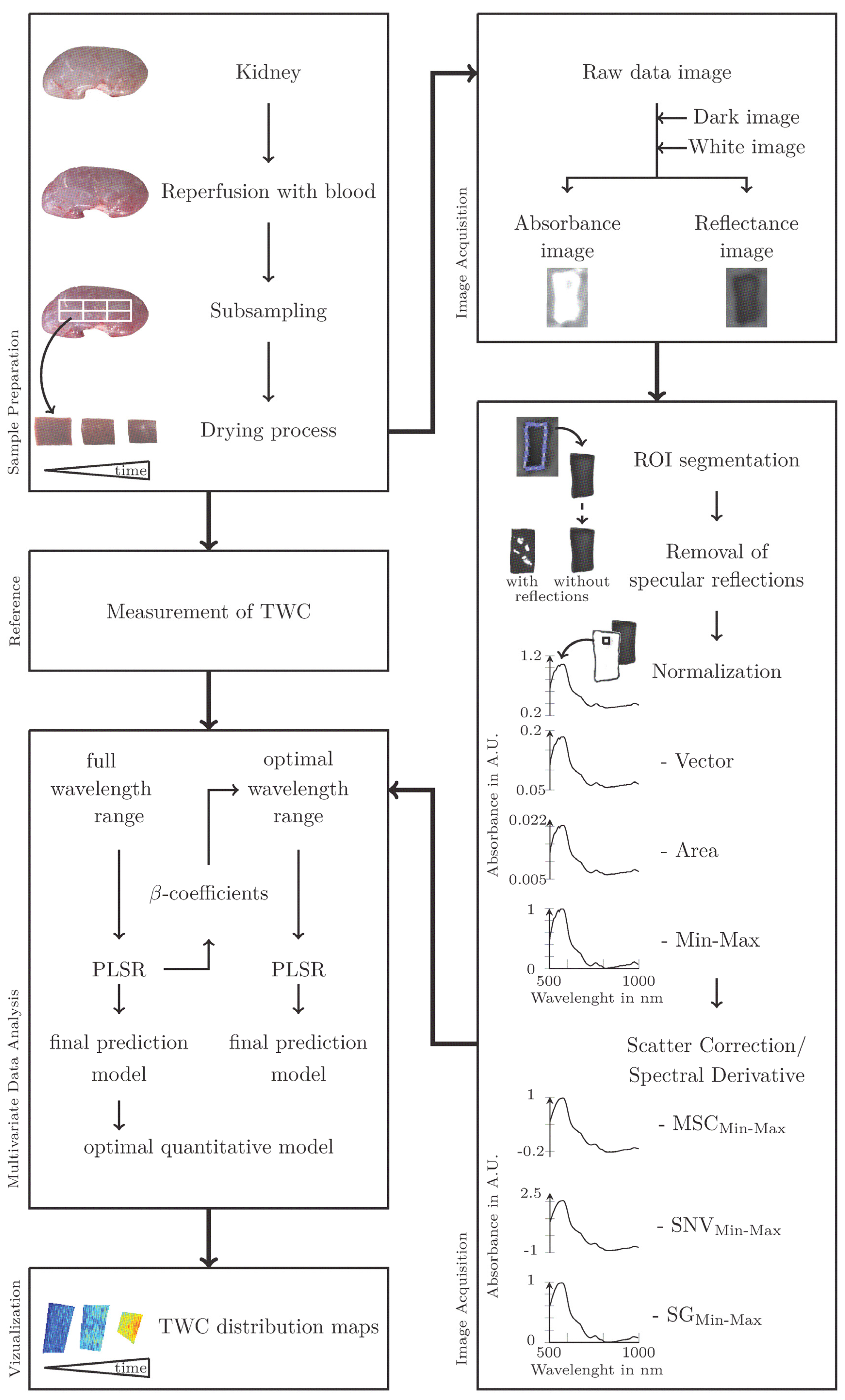
2.1. Sampling Strategy and Preparation

A suitable sampling strategy is essential to fulfill various criteria of reproducibility, value range, and variance within the sample. To meet these requirements, we have recorded a suitable dataset according to the American Society for Testing and Materials (ASTM) standard practice E1655-05 [41]. In the following, the mentioned criteria are described in detail. To develop a reliable calibration model, the characteristics of the samples included in this model have to correspond to the characteristics of samples analyzed in the future. Therefore, whole blood reperfusion of the porcine kidneys was performed before sample collection and the subsequent determination of the TWC. Another criterion was that the training dataset had to cover the range of TWC in kidney tissue during NMP. Here, the water content could vary due to osmotic imbalances caused by ischemia/reperfusion damage [17,18]. To obtain representative values of TWC in non-physiological conditions, some kidney samples were additionally exposed to different drying times. Furthermore, the TWC may vary within the same kidney leading to deviations from the mean water content. Therefore, sub-sampling was performed to obtain a wide range of TWC values for the calibration model. For each kidney, samples were taken from six different regions in order to include possible spatial divergences.

For this study, 23 kidneys from female German Landrace slaughterhouse pigs were used. The pigs’ selection criteria were homogenous age (six months), weight (100–120 kg), and origin (local slaughterhouse with 10–15 pigs slaughtered per week) as well as health (inspected by an official veterinarian). Up to six kidneys per week were analyzed. A detailed description of blood and organ removal as well as storage can be found in [25].

Each kidney was filled with temperatured autologous whole blood (T_Blood = 37 ± 0.5 °C, hematocrit = 32 ± 5%) and cut into six rectangular pieces with the respective dimensions of 3 cm × 1 cm × 0.5 cm (length × width × thickness), resulting in a weight of 2 ± 0.05 g. The prepared tissue specimens were analyzed following the Association of Official Analytical Chemists (AOAC) standard method for moisture analysis 950.46 B, where the samples were dried at 102 °C for 18 h [42]. Generally, the TWC of porcine kidneys ranged from 81.5 to 89.3% (shown in

Table 1. Drying characteristics of kidney tissue using the oven drying method.

Drying Time in Min	No. Kidneys	Tissue Water Content in %
		Mean	Standard Deviation	Range
0	23	84.16	1.63	81.52–89.27
10	6	68.75	4.36	54.24–75.07
20	6	57.43	5.12	44.27–67.32

). In order to predict this TWC range as good as possible for future applications during NMP, a majority of the samples of the training dataset was concentrated on this range. In addition, to reflect non-physiological conditions, the TWC was artificially reduced. Thus, some kidneys were also analyzed after 10 and 20 min of drying time.

2.2. Measurement of the Tissue Water Content

Following the standard practice AOAC 950.46 B [42], the TWC (in %) of each kidney sample was calculated as the percentage of weight loss using the oven drying method:

$$\mathrm{Tissue} \mathrm{water} \mathrm{content} = 100- \frac{\mathrm{w} - \mathrm{d}}{\mathrm{w}},$$

(1)

where w is the weight of the wet sample (in g) and d the weight of the dry sample (in g). The percentage of water was expressed as the reference water content value of each sample for subsequent data analysis. Table 1 shows the relevant statistics of TWC for the samples.

2.3. Hyperspectral Imaging System

The HSI system comprised two main components: the HSI camera and the illumination unit. This study’s hyperspectral camera was a line-scan hyperspectral camera (TIVITA Tissue Camera, Diaspective Vision GmbH, Am Salzhaff, Germany), based on the push broom scanning method. This camera contained a CMOS sensor (AR0130CS, On Semiconductor Corp., Phoenix, AZ, USA) with a resolution of 1280 pixels × 960 pixels and was equipped with an AZURE Photonics 2/3″ 12 mm objective lens (AZURE Photonics U.S.A., Inc., San Ramon, CA, USA). In order to acquire a focused image, the distance between objective and kidney sample surface was adjusted to 46 cm. The HSI system covers the spectral range of 500–995 nm with a spectral resolution of 5 nm. The illumination unit contained six 20 W quartz-tungsten-halogen spots (OSRAM 41,861 Decostar 51 ALU, Osram GmbH, München, Germany) with an aluminum reflector for homogeneous illumination of the field of view (FOV). A laptop (ThinkPad W530, Lenovo GmbH, Stuttgart, Germany) with the TIVITA Suite software 0.6.1.4 (Diaspective Vision GmbH, Am Salzhaff, Germany) was used exclusively for image acquisition. This software reduced the hyperspectral data cube to 640 px (x-dimension) × 480 px (y-dimension) × 100 wavelengths (λ-dimension). Further technical information of the HSI camera system can be found in previously published literature [24].

A custom written MATLAB code (MATLAB R2018b, The MathWorks, Inc., Natick, MA, USA) was used to analyze the HSI data. The workflow of the main steps in the current research is illustrated in Figure 1.

2.4. Image Acquisition and Data Correction

For each experiment, a dark current image I_DARKx,y,λ and a white reference image I_WHITEx,y,λ were recorded to correct the raw intensity images I_RAWx,y,λ of the sample. I_DARKx,y,λ was obtained by closing the camera shutter and switching off the light source when capturing the HSI image. I_WHITEx,y,λ was acquired with a reflectance standard (Zenith Polymer Target SG3210, SphereOptics GmbH, Germany) placed in the FOV.

From the raw intensity image I_RAWx,y,λ, both the reflectance image I_REFLx,y,λ (see Equation (2)), as well as the absorbance image I_ABSx,y,λ (see Equation (3)), were calculated [19]:

$${\mathrm{I}}_{\mathrm{REFL} \mathrm{x},\mathrm{y},\mathsf{\lambda }}= \frac{{\mathrm{I}}_{\mathrm{RAW} \mathrm{x},\mathrm{y},\mathsf{\lambda }} -{ \mathrm{I}}_{\mathrm{DARK} \mathrm{x},\mathrm{y},\mathsf{\lambda }}}{{\mathrm{I}}_{\mathrm{WHITE} \mathrm{x},\mathrm{y},\mathsf{\lambda }} -{ \mathrm{I}}_{\mathrm{DARK} \mathrm{x},\mathrm{y},\mathsf{\lambda }}},$$

(2)

$${\mathrm{I}}_{\mathrm{ABS} \mathrm{x},\mathrm{y},\mathsf{\lambda }}= -\lg {\mathrm{I}}_{\mathrm{REFL} \mathrm{x},\mathrm{y},\mathsf{\lambda }}.$$

(3)

HSI data were collected from the kidneys before and during the drying process.

2.5. Data Preprocessing

Several image preprocessing steps are necessary before the quantitative data analysis of kidney samples’ HSI images. These aim to remove irrelevant information, noise, and physical phenomena from the data to improve the subsequent multivariate data analysis. The data preprocessing includes the following steps:

Step 1: ROI Segmentation

The segmentation process removes pixels of the background from the hyperspectral data cube, which do not contain chemical information about the sample. The determination of region-of-interest (ROI), representing the sample within the hyperspectral images, was performed by manual ROI selection using the roipoly function of MATLAB.

Step 2: Removal of Specular Reflections

Within the ROI, specular reflections can occur and appear as bright spots in absorbance images. These are caused by the presence of moisture on the kidney’s surface, which acts like a mirror reflecting the light of the illumination system. Since specular reflections overlap the sample’s actual chemical properties, they can also influence the subsequent data analysis and must, therefore, be removed. For data preprocessing, absorbance images were used to determine the pixels affected by specular reflections, which cause low intensities and can, therefore, be detected and segmented using a threshold-based method. The elimination of 10% of the darkest pixels in the absorbance image was achieved with the Thresholding Tool implemented in MATLAB [43].

Step 3: Spectral Normalization

For a reasonable comparison of spectra, it is useful to scale their values to the same range by normalization. In order to compare the influence of normalization method on the prediction performance of the model, three different methods (min-max, area, and vector normalization) were applied to the spectra [44]. Min-max normalization is a common method to preprocess data. For each spectrum, the minimum value of that spectrum was set to 0, and the maximum value to 1, while the other values are distributed accordingly. The min-max normalized absorbance and reflectance image were calculated as follows:

$${\mathrm{I}}_{\mathrm{ABS} \mathrm{x},\mathrm{y},\mathsf{\lambda }\mathrm{norm}}= \frac{{\mathrm{I}}_{\mathrm{ABS} \mathrm{x},\mathrm{y},\mathsf{\lambda }}- \mathrm{Min}({\mathrm{I}}_{\mathrm{ABS} \mathrm{x},\mathrm{y},\mathsf{\lambda }})}{\mathrm{Max}({\mathrm{I}}_{\mathrm{ABS} \mathrm{x},\mathrm{y},\mathsf{\lambda }})- \mathrm{Min}({\mathrm{I}}_{\mathrm{ABS} \mathrm{x},\mathrm{y},\mathsf{\lambda }})} ,$$

(4)

$${\mathrm{I}}_{\mathrm{REFL} \mathrm{x},\mathrm{y},\mathsf{\lambda }\mathrm{norm}}= \frac{{\mathrm{I}}_{\mathrm{REFL} \mathrm{x},\mathrm{y},\mathsf{\lambda }}- \mathrm{Min}({\mathrm{I}}_{\mathrm{REFL} \mathrm{x},\mathrm{y},\mathsf{\lambda }})}{\mathrm{Max}({\mathrm{I}}_{\mathrm{REFL} \mathrm{x},\mathrm{y},\mathsf{\lambda }})- \mathrm{Min}({\mathrm{I}}_{\mathrm{REFL} \mathrm{x},\mathrm{y},\mathsf{\lambda }})} .$$

(5)

In the second approach, the area normalization is calculated by dividing each spectrum by a constant that corresponds to the sum of all intensities over the wavelength range (see Equations (6) and (7)):

$${\mathrm{I}}_{\mathrm{ABS} \mathrm{x},\mathrm{y},\mathsf{\lambda }\mathrm{norm}}= \frac{{\mathrm{I}}_{\mathrm{ABS} \mathrm{x},\mathrm{y},\mathsf{\lambda }}}{{\displaystyle \sum }{\mathrm{I}}_{\mathrm{ABS} \mathrm{x},\mathrm{y},\mathsf{\lambda }}},$$

(6)

$${\mathrm{I}}_{\mathrm{REFL} \mathrm{x},\mathrm{y},\mathsf{\lambda }\mathrm{norm}}= \frac{{\mathrm{I}}_{\mathrm{REFL} \mathrm{x},\mathrm{y},\mathsf{\lambda }}}{{\displaystyle \sum }{\mathrm{I}}_{\mathrm{REFL} \mathrm{x},\mathrm{y},\mathsf{\lambda }}}.$$

(7)

Vector normalization, in which the spectrum is considered a vector and each vector value is divided by the square root of the sum of the squares of all vector values, is calculated as follows:

$${\mathrm{I}}_{\mathrm{ABS} \mathrm{x},\mathrm{y},\mathsf{\lambda }\mathrm{norm}}= \frac{{\mathrm{I}}_{\mathrm{ABS} \mathrm{x},\mathrm{y},\mathsf{\lambda }}}{\sqrt{{\displaystyle \sum }{\mathrm{I}}_{\mathrm{ABS} \mathrm{x},\mathrm{y},\mathsf{\lambda }}{}^2}},$$

(8)

$${\mathrm{I}}_{\mathrm{REFL} \mathrm{x},\mathrm{y},\mathsf{\lambda }\mathrm{norm}}= \frac{{\mathrm{I}}_{\mathrm{REFL} \mathrm{x},\mathrm{y},\mathsf{\lambda }}}{\sqrt{{\displaystyle \sum }{\mathrm{I}}_{\mathrm{REFL} \mathrm{x},\mathrm{y},\mathsf{\lambda }}{}^2}}.$$

(9)

Step 4: Scatter Correction and Spectral Derivates

Three different methods were considered for noise correction to reduce the influence of distorted spectra on the prediction model. Two methods—multiplicative scatter correction (MSC) and standard normal variate (SNV)—for scatter correction, and the Savitzky–Golay method (SG) for spectral derivation [45]. All preceding methods intend to remove distorted signal portions that would otherwise impede the construction of a valid prediction model.

MSC is the most commonly used scatter correction method for NIR data. It estimates influences (e.g., light scattering) for each sample relative to the entire mean spectrum. Scatter correction by MSC was calculated as follows:

$${\mathrm{x}}_{\mathrm{org}}={\mathrm{b}}_0+{\mathrm{b}}_{\mathrm{ref},1 }·{ \mathrm{x}}_{\mathrm{ref}}+\mathrm{e} ,$$

(10)

$${\mathrm{x}}_{\mathrm{corr}}= \frac{{\mathrm{x}}_{\mathrm{org}} -{ \mathrm{b}}_0}{{\mathrm{b}}_{\mathrm{ref},1}},$$

(11)

where x_org is one original sample spectra measured by the HSI camera, x_ref is a reference spectrum used for preprocessing of the entire dataset, e is the unmodeled part of x_org, x_corr is the corrected spectra, and b₀ and b_ref,1 are scalar parameters, which differ for each sample [45].

The SNV method, a related method to MSC, is the second most applied method for scatter correction of NIR data and is given in the following equation:

$${\mathrm{x}}_{\mathrm{corr}}= \frac{{\mathrm{x}}_{\mathrm{org}} -{ \mathrm{a}}_0}{{\mathrm{a}}_1},$$

(12)

where a₀ is the average value of the sample spectrum to be corrected, and a₁ is the standard deviation of the sample-spectrum [45].

SG for spectral derivation, which includes a smoothing step, was applied with MATLAB’s Sgolayfilt function. The used filter worked with a polynomial order of 3 and a frame length of 11.

2.6. Multivariate Data Analysis

2.6.1. Partial Least Squares Regression (PLSR)

In order to create quantitative models between the preprocessed spectral data and the measured reference values of TWC, PLSR method was applied for multivariate data analysis. PLSR is a commonly used and reliable analytical tool for spectra data processing and predictive model development [46]. The multivariate data analysis was performed with the plsregress function of MATLAB. The PLSR model was calculated as follows:

$$\mathrm{X}={\mathrm{TP}}^{\mathrm{T}}+\mathrm{E} ,$$

(13)

$$\mathrm{Y}={\mathrm{UQ}}^{\mathrm{T}}+\mathrm{F} ,$$

(14)

where the spectral data matrix X is decomposed into the score matrix T, loading matrix P, and error matrix E. The reference values matrix Y is decomposed into the score matrix U, loading matrix Q, and error matrix F [46].

PLSR estimates latent variables (LV) that describe the maximum covariance between the spectral data and the measured TWC (response variables). The optimal number of LVs was determined using the minimum predicted by the root mean square error (RMSE) method during cross-validation.

2.6.2. Data Partition

A total of 208 samples were collected to ensure an appropriate range of TWC values. The dataset was manually divided into a training set consisting of 172 samples (83%) and a test set consisting of 36 samples (17%). The statistical values of TWC in the training and the test set for this study are shown in

Table 2. Reference values of TWC in %.

Statistics	Training Set n = 172 (19 Kidneys)	Test Set n = 36 (4 Kidneys)
Mean	76.83	77.06
Standard deviation	10.97	11.42
Maximum	89.27	88.01
Minimum	44.27	46.80

.

The PLSR models were built with the training data using a full cross-validation method (leave-one-out), in which one validation set was removed at one time from the training set until all samples have been removed once. The PLSR model was then established based on the remaining samples of the training set. It should be noted that six tissue samples were taken from each kidney. The samples from one kidney were selected together as one validation set from the training set, as these samples are not independent of each other. The number of LVs and the accuracy of PLSR models in training were estimated by the root-mean-square error resulted from cross-validation (RMSECV). Finally, this established model was used to predict the TWC in the independent test set and evaluate the performance of the algorithm. A good PLSR prediction model is characterized by a high coefficient of determination in prediction (R_P²) and a low root-mean-square error of prediction (RMSEP).

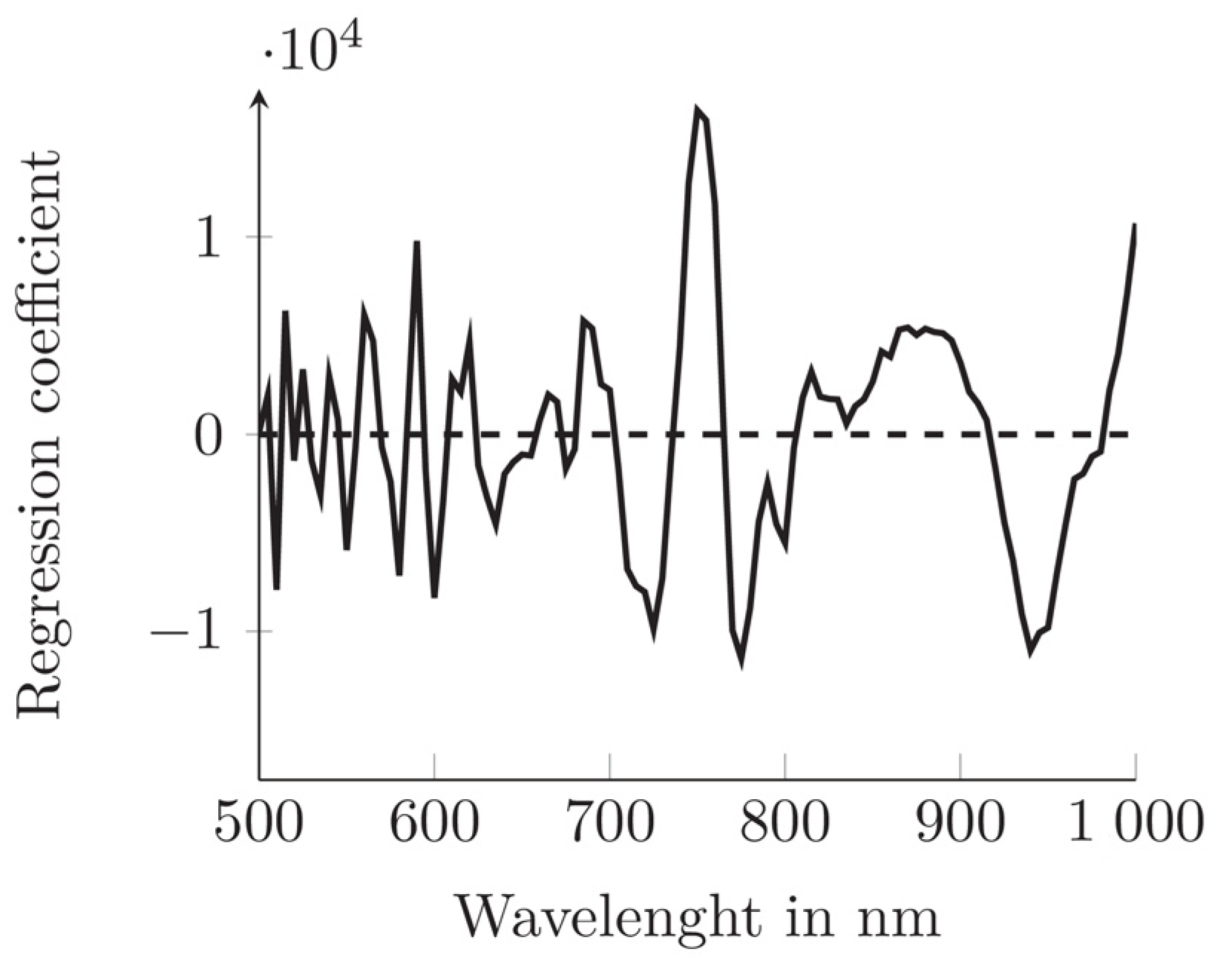
2.7. Optimal Wavelengths Selection Strategy

The kidney’s spectra data were first analyzed in the full spectra range of 500–995 nm containing 100 wavelengths.

In hyperspectral image analysis, selecting the most influential spectral wavelength instead of using the whole spectrum showed better predictive results in some cases [47,48]. The cause could be explained by bands containing noise or irrelevant information for data analysis. However, there is no gold standard for selecting significant wavelengths from the whole spectrum [49]. In this study, weighted PLS regression coefficients, also called β-coefficients from the PLSR models, were used to estimate the most influential wavelengths for TWC prediction. The method is based on the principle of calculating β-coefficients corresponding to the full-spectrum model. The wavelengths with the highest absolute values of regression coefficients were chosen and used for the development of new PLSR models.

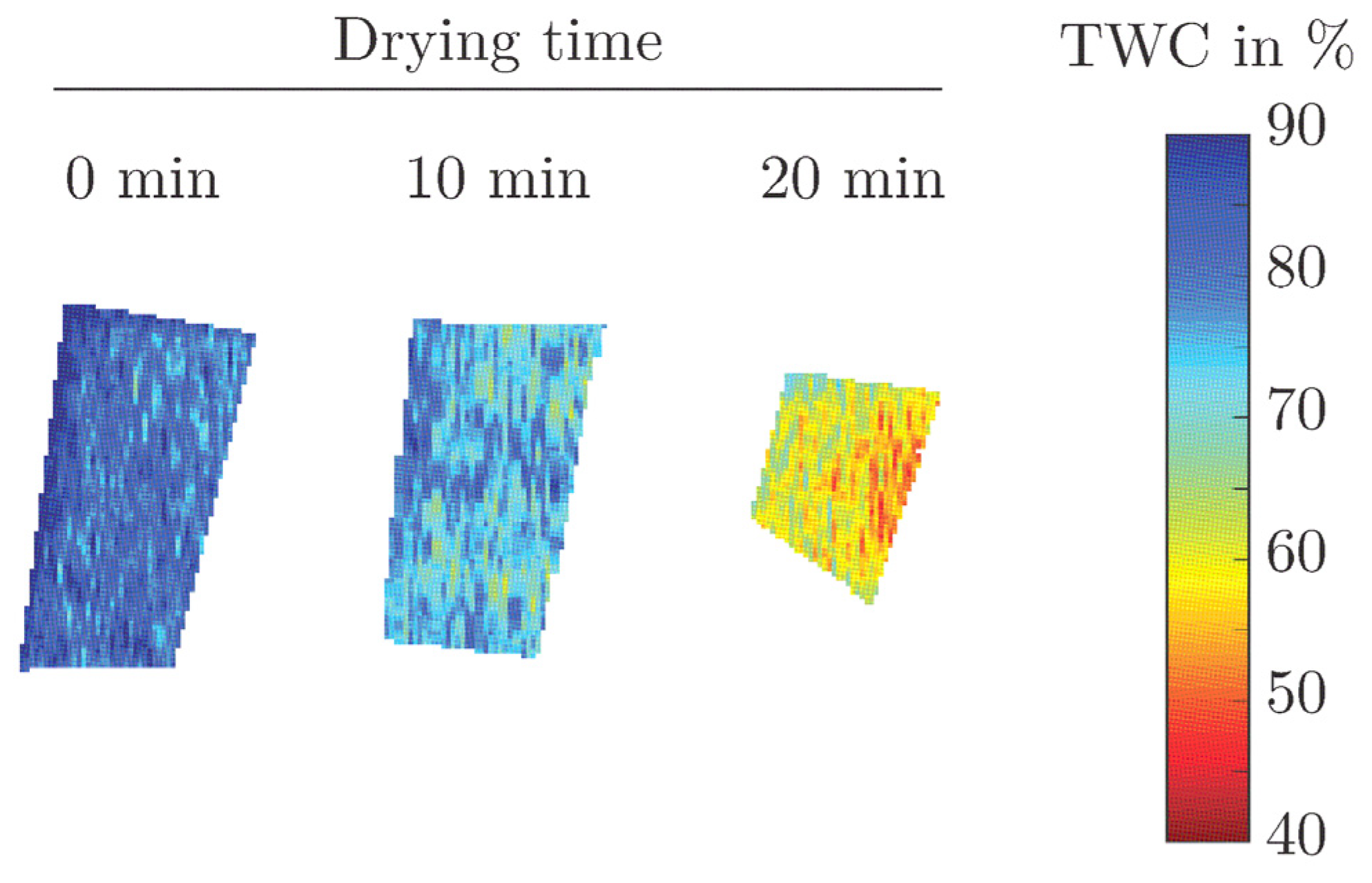
2.8. Visualization of Water Content

Using HSI, the spatial distribution of water within a sample can be visualized. TWC maps from the kidney samples were obtained by multiplying the β-coefficients from the PLSR model with the spectrum of each pixel in the image. The optimal multivariate model was chosen to display and map each pixel of the hyperspectral image to predict water content in the kidney samples. The resulting water distribution map is visualized with a linear color bar, representing the predicted values of every pixel into different colors. High TWC is shown in blue, and those with low water values are shown in red. For all visualization routines, the Colormap function of MATLAB was used.

3. Results

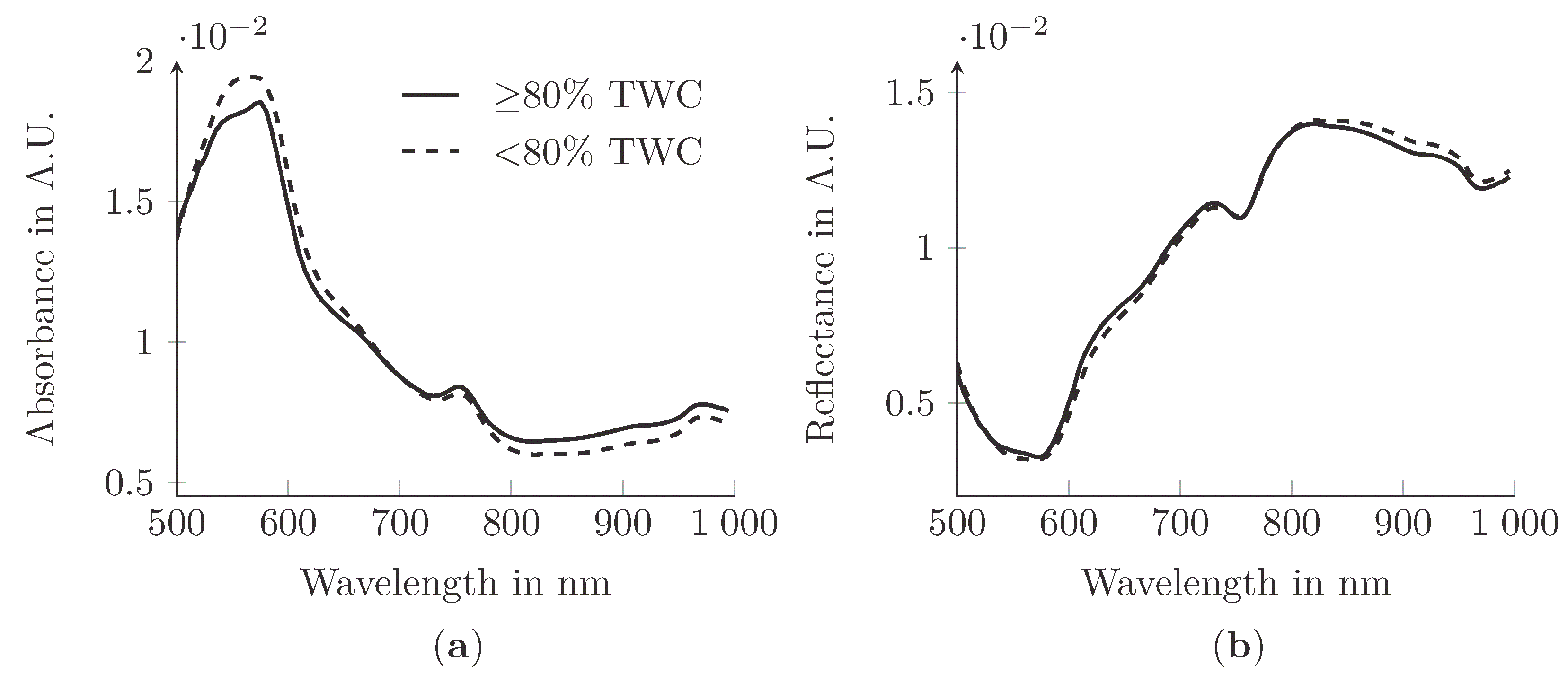
3.1. Spectral Features of Porcine Kidneys in the Spectral Range of 500 to 995 nm

In this study, kidneys were examined with a TWC between 44.27% and 89.27% (see Table 1). The averaged absorbance and reflectance spectra of porcine kidney samples with physiological TWCs ≥ 80% and non-physiological TWCs < 80% in the wavelength range between 500 and 995 nm are shown in Figure 2. The spectra were area normalized and smoothed.

Kidney spectra were characterized by the tissue chromophores hemoglobin, lipids, and water, which absorb in the visible/near-infrared (VIS/NIR) range. This spectral region is related to several broadband peaks and fundamental vibrations. The main absorption of hemoglobin occurred in the wavelength range between 500 and 800 nm, which was caused by the spectroscopic properties of porphyrins [50]. For lipids, the absorption peak at 930 nm was associated with the third overtone C–H section in the methylene group of lipids [39]. The most characteristic absorption features of water consisted of two regions: an absorbance peak around 750 nm and around 970 nm assigned to the third and second overtones of O–H stretching [37].

Although there was a trend that samples with high TWC showed high absorbance in the prominent peaks, it can be assumed that other chromophores partly overlap these. Employing a simple linear regression method would, therefore, not result in a reliable prediction of TWC. Consequently, the use of multivariate modeling is a prerequisite for the extraction of quantitative information from the spectra of kidney samples with respect to the water content.

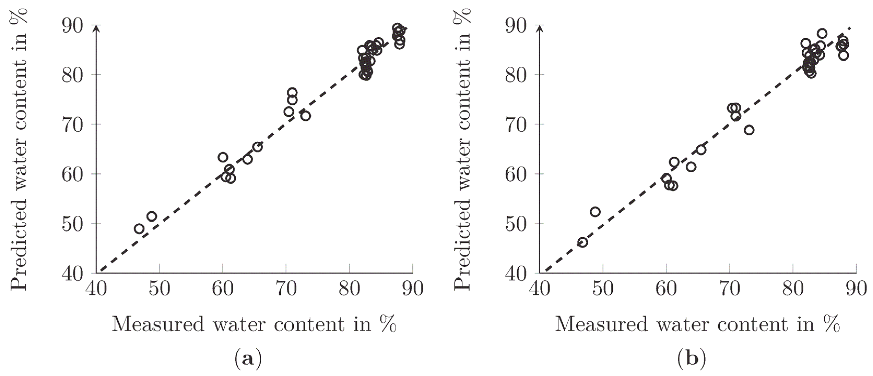
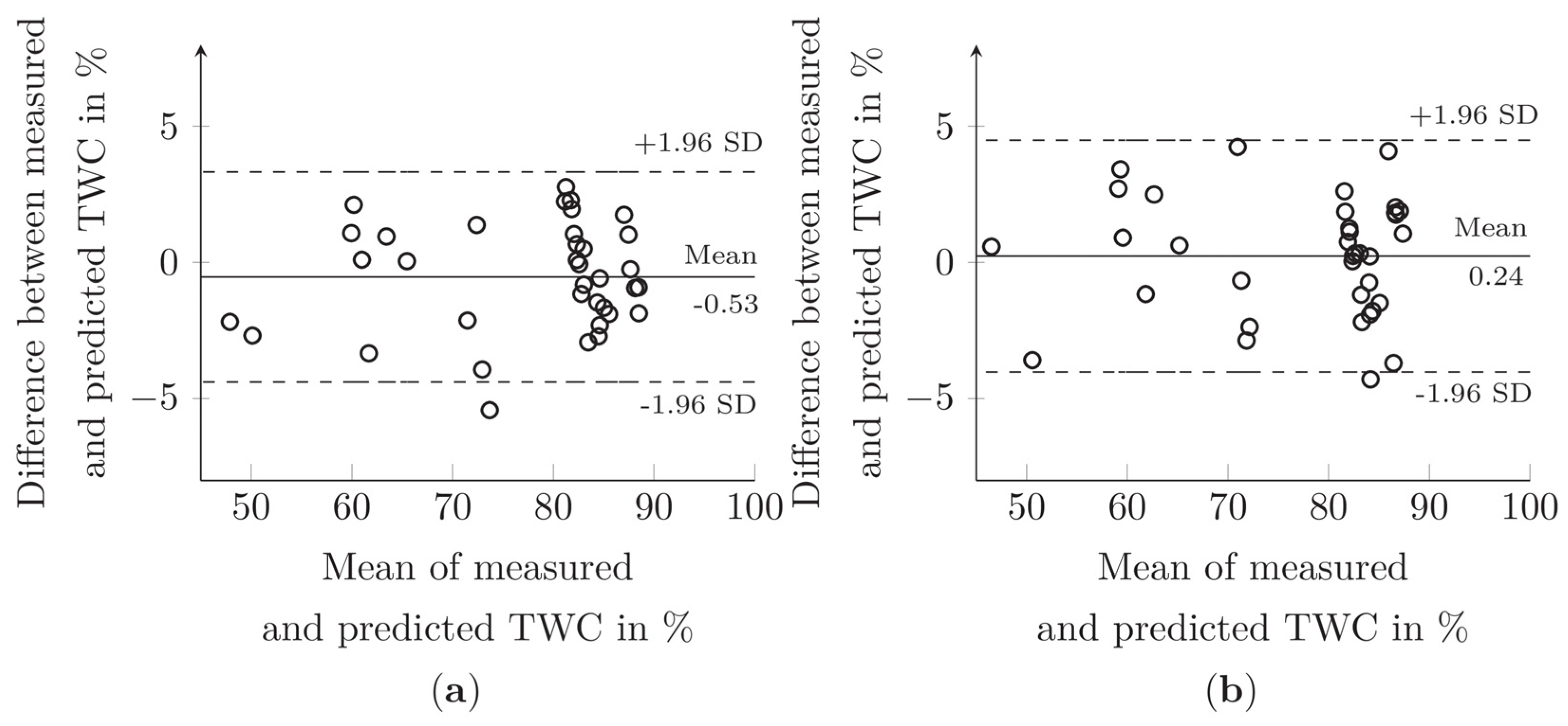
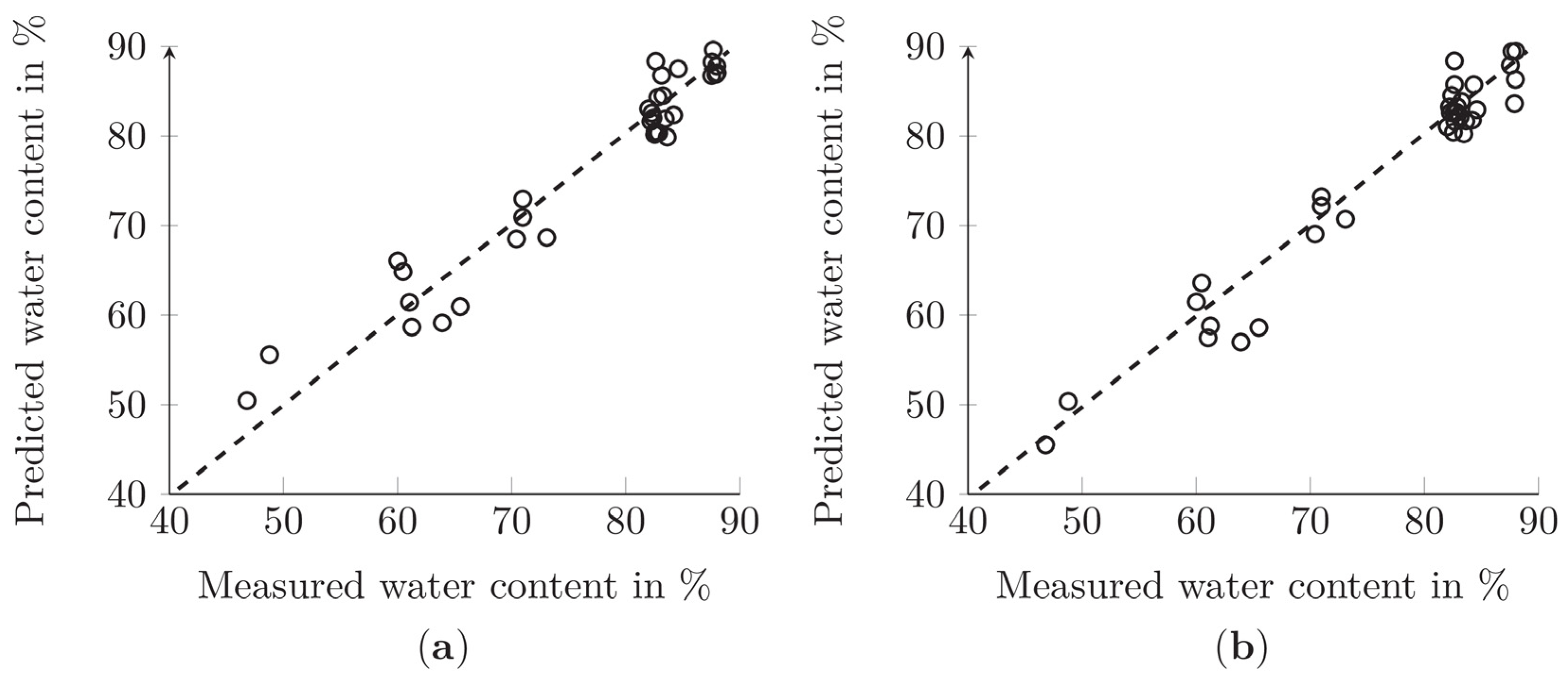
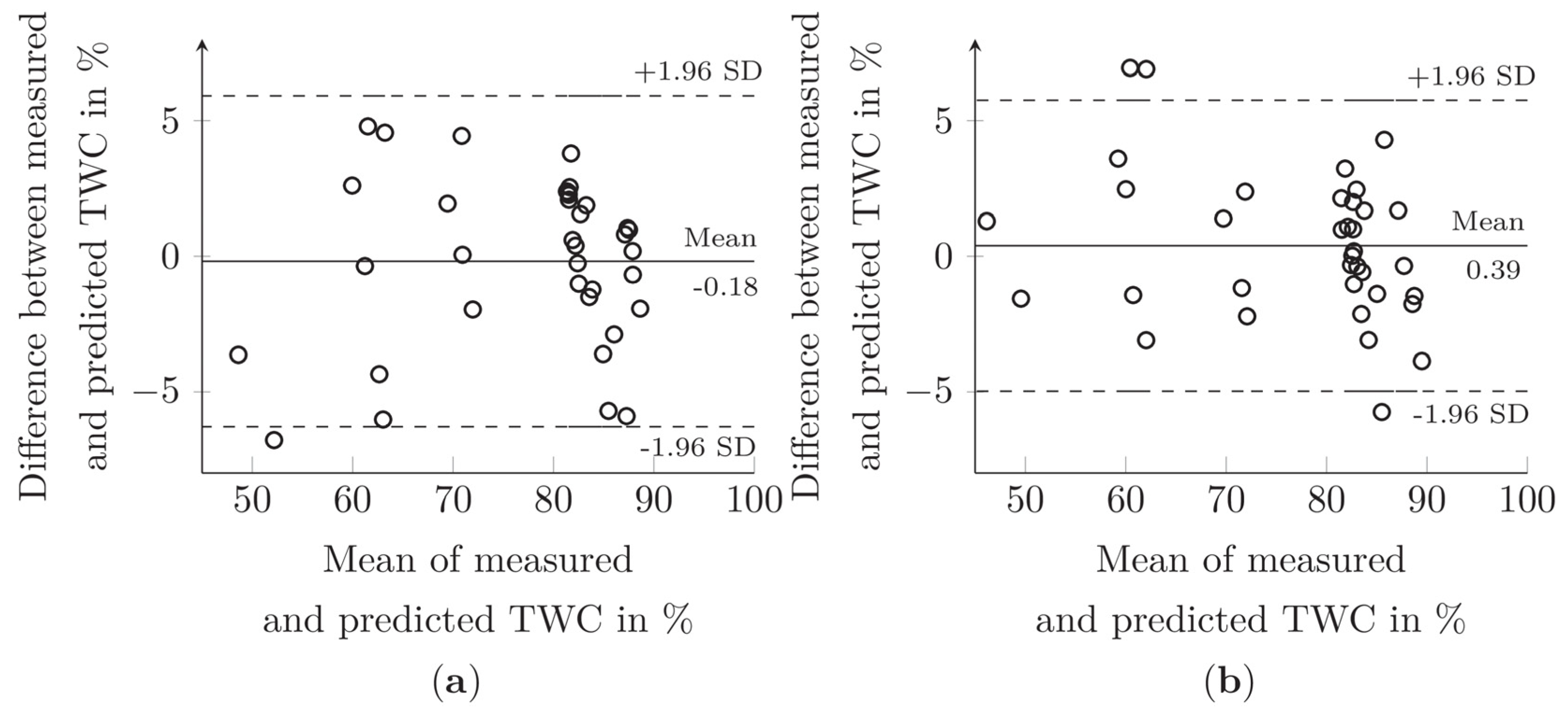
3.2. Prediction of Water Content Using Full Spectral Range

In order to investigate which data are best suited for the prediction model, first the absorbance and reflectance data in the entire spectral range between 500 and 995 nm were considered (100 wavelengths). The performances of the PLSR models were evaluated using several variants of spectral preprocessing methods (normalization followed by scatter correction or spectral derivation), which influenced the final predictive power (shown in

Table 3. Performance of PLSR for prediction TWC based on 100 wavelengths.

Normalization	Filter	LV’s	Validation Model	Prediction Model
			RMSECV	R2P	RMSEP
Absorbance
Min-Max	-	17	3.570	0.912	3.339
	SNV	17	3.800	0.904	3.498
	MSC	26	6.220	0.939	2.774
	SG	17	3.557	0.905	3.463
Area	-	21	4.628	0.968	2.026
	SNV	17	3.961	0.901	3.542
	MSC	3	6.320	0.876	3.970
	SG	14	3.207	0.968	2.016
Vector	-	15	3.285	0.960	2.263
	SNV	17	3.995	0.902	3.529
	MSC	25	5.949	0.926	3.068
	SG	15	3.085	0.957	2.343
Reflectance
Min-Max	-	17	3.048	0.961	2.225
	SNV	23	3.028	0.955	2.401
	MSC	8	5.620	0.795	5.102
	SG	17	2.795	0.963	2.162
Area	-	16	3.026	0.958	2.318
	SNV	16	3.095	0.950	2.511
	MSC	21	8.965	0.957	2.325
	SG	15	2.928	0.942	2.704
Vector	-	17	3.070	0.959	2.274
	SNV	16	3.095	0.950	2.511
	MSC	19	6.919	0.963	2.155
	SG	16	2.925	0.942	2.714

). The absorbance images of the kidney samples preprocessed by SG smoothing following area normalization and the reflectance images preprocessed by MSC following vector normalization exhibited the best results with R_P² values of 0.968 and 0.963, as well as RMSEP values of 2.016 and 2.155.

Figure 3 shows the reference versus predicted value plots for TWC using the optimal PLSR models. Both absorbance and reflectance data sets showed promising results.

The Bland–Altman method was used to evaluate the differences between the measured and the predicted TWC values (see Figure 4). For both absorbance and reflectance, there was no average discrepancy between methods and no trend of the difference in relation to the mean. The limits of agreement were [−4.39; +3.32]% for absorbance and [−4.02; +4.49]% for reflectance.

3.3. Multivariate Statistical Analysis Based on Optimal Wavelengths

The selection of the most influential wavelengths was performed by calculating the β-coefficients derived from the PLSR models. Figure 5 shows the regression coefficients of the best PLSR model, an absorbance model. In general, wavelengths with values close to zero do not contribute to the explanation of the chemical variation. High positive values are positively correlated with the dependent variable water; negative values are negatively correlated. The spectral range between 500 and 700 nm did not allow a definite assignment. A maximum was found at 750 nm. This peak is characterized by the O-H stretching second overtone of water and the spectral properties of deoxyhemoglobin. Due to the overlap of the water peak with the hemoglobin peak [51], the wavelength range of hemoglobin absorption (500–800 nm) is not considered for a future model. The influence of lipid absorption in the 930 nm wavelength range is compensated by a minimum of the regression coefficient. To avoid possible influences on the model by image sensor noise, no wavelengths above 980 nm are used. Since the β-regression coefficient method did not show clear minima and maxima, the range of 800–980 nm (37 wavelengths) is selected as an optimized wavelength range.

The performance of the wavelength-adapted model for TWC prediction by HSI is represented in

Table 4. Performance of PLSR for prediction TWC based on 37 wavelengths.

Normalization	Filter	LV’s	Validation Model	Prediction Model
			RMSECV	R2P	RMSEP
Absorbance
Min-Max	-	20	4.111	0.894	3.669
	SNV	7	4.486	0.925	3.075
	MSC	10	7.965	0.759	5.527
	SG	14	3.868	0.904	3.481
Area	-	12	5.072	0.904	3.494
	SNV	12	3.807	0.886	3.801
	MSC	4	8.610	0.824	4.725
	SG	20	3.854	0.923	3.122
Vector	-	13	3.584	0.914	3.295
	SNV	12	3.789	0.887	3.779
	MSC	4	7.195	0.490	8.0441
	SG	17	3.837	0.921	3.159
Reflectance
Min-Max	-	11	3.544	0.919	3.202
	SNV	13	3.698	0.911	3.352
	MSC	7	7.861	0.898	3.593
	SG	13	3.752	0.929	3.001
Area	-	11	3.485	0.941	3.202
	SNV	13	3.687	0.913	3.327
	MSC	1	9.641	0.201	10.065
	SG	13	3.896	0.943	2.699
Vector	-	12	3.416	0.937	2.819
	SNV	13	3.687	0.913	3.327
	MSC	15	8.160	0.852	4.336
	SG	10	3.828	0.920	3.180

. The best prediction results were obtained with R_P² values of 0.925 and 0.941, as well as RMSEP values of 3.075 and 3.202 for the absorbance data preprocessed with min-max normalization following SNV and reflectance data with area normalization.

The relationship between measured versus predicted TWC values using the optimal PLSR models is shown in Figure 6. The absorbance and the reflectance models showed promising but still slightly worse results than the full spectral models presented above.

Figure 7 shows the Bland–Altman plots for evaluating the differences between the measured and the predicted TWC values. There was no average discrepancy between the methods, as well as no trend of the difference in relation to the mean observed for absorbance and reflectance, respectively. The limits of agreement were [−6.29; +5.92]% for absorbance and [−4.97; +5.76]% for reflectance.

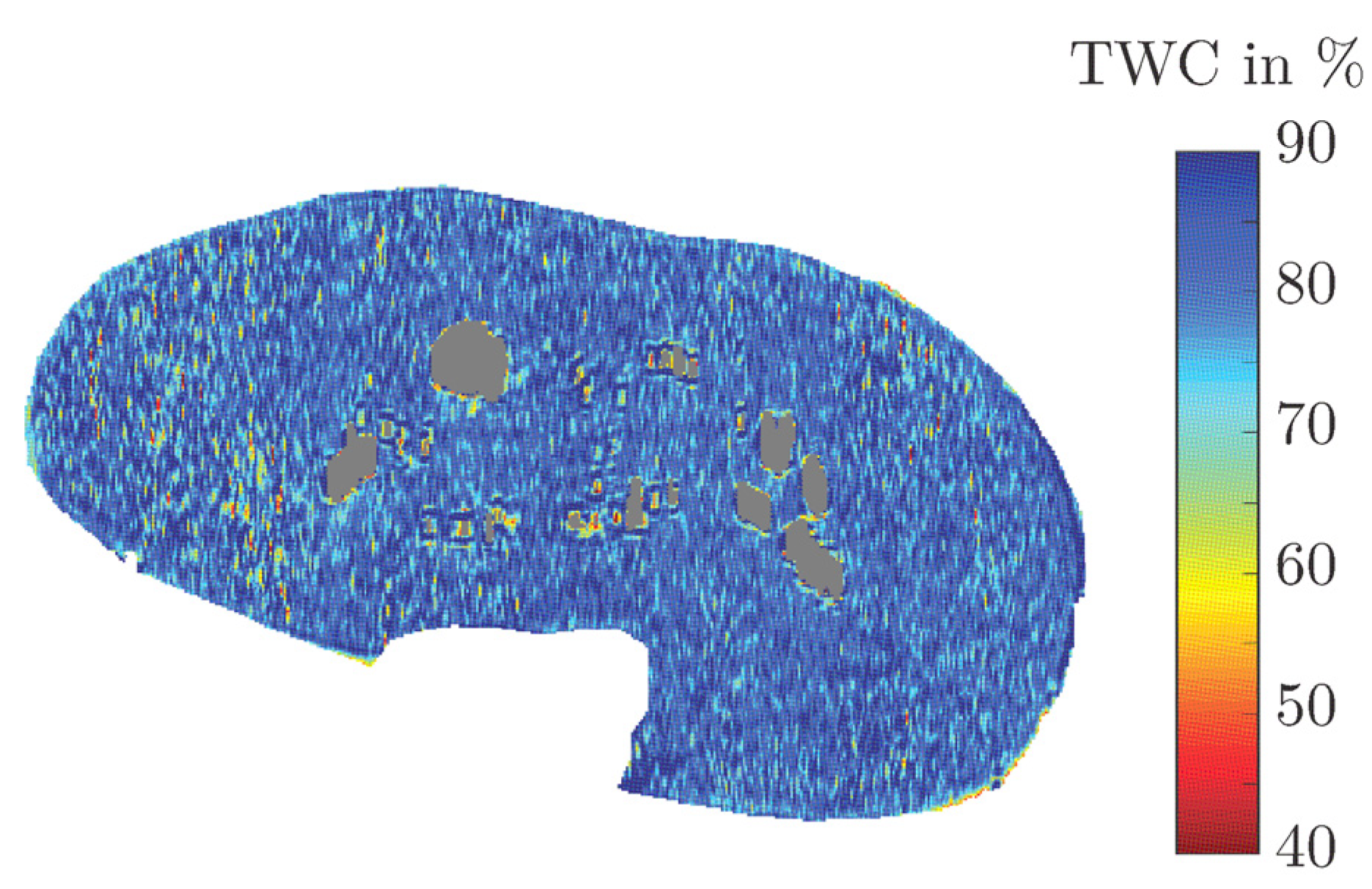
3.4. Visualization of Water Content Distribution

The PLSR model that achieved the best results in TWC prediction on the test data (full wavelength range absorbance spectra preprocessed with area normalization and SG) was employed to determine the TWC within the kidney tissue during the drying process. Figure 8 illustrates the two-dimensional distribution of TWC in one sample for three consecutive times. Due to the drying process, the kidney sample changed in size and shape.

Before the drying process started, the tissue had a physiological TWC of ≥80%, which decreased with the drying process duration. The estimated values, based on the mean of the single-pixel predictions, for the TWC at the beginning of the drying process, after 10 min and after 20 min (82.30%, 74.91%, and 59.40%) correspond well to the TWC determined by the reference method (82.39%, 70.98%, and 60.02%).

Finally, the TWC distribution map of a kidney during NMP is shown in Figure 9. Areas on the surface of the kidney without information on the TWC were assigned to specular reflections. The measured and the predicted TWC for the kidney were 82.76% and 81.95%, respectively.

4. Discussion

This study demonstrated the feasibility of HSI in combination with PLSR to assess the TWC in porcine kidneys during NMP. Here, the wavelength range of 500 to 995 nm could be used to identify water-related characteristics of kidney tissue. PLSR models derived from the analysis of a suitable dataset were applied to quantify TWC. A model based on the absorbance spectra of the full wavelength range yielded the best performance in predicting the TWC and was used to visualize the TWC distribution of the kidneys’ surface.

4.1. Hyperspectral Imaging for Spectral Characterization of Kidney Tissue in the VIS/NIR Region

HSI enables fast and non-invasive measurement of tissue properties in, e.g., medical applications. Using this technique, information about physiological and pathological tissue characteristics can be obtained [20,21,22,23,24,25]. Water-specific tissue features of the kidney were assessed using HSI in the wavelength range between 500 and 995 nm. By predicting the TWC, tissue-related damage during ex vivo preservation could be detected in the future.

Depending on the medical application, the analyzed HSI spectral range varies between 400 and 2500 nm. However, tissue characterization is preferably performed in the optical window between 600 and 1000 nm. In this wavelength range, the amount of VIS/NIR light absorbed by the tissue is limited, which allows a high penetration depth of the light into the tissue [19]. In the optical window, the main absorbers are melanin, hemoglobin, lipids, and water [37,39,50]. Since the organic samples’ composition is complex, the absorption bands tend to be broad and generally overlap in different parts of the NIR range [51]. Two water absorption peaks were observed at 760 and 970 nm [37]. Therefore, the quantification of the TWC in medical applications or food analysis was successfully performed by using the wavelength range of 400–1000 nm [27,37,38,47,52,53].

The application of HSI is limited by the low penetration depth of the propagating light into the tissue. Depending on the wavelength, the illumination has a penetration depth of only a few millimeters [54]. In the kidney, the main metabolic activity is concentrated in the cortex region [55,56]. An impairment of the kidney quality caused by IRI, for example, could have a decisive influence on this external organ region and would, therefore, have a considerable impact on the physiological condition and composition of the kidney. Consequently, metabolic-related kidney injury could be detected with HSI.

4.2. Partial Least Square Regression for Prediction of the TWC in Kidneys

In this study, PLSR analysis was used to quantify the TWC by simulating an application during normothermic preservation of ex vivo kidneys. In medical application, PLSR has not yet been used to determine the TWC. Here, we proposed the suitability and effectiveness of this analytical tool to predict the TWC in kidney tissue during a non-invasive application. For a TWC range between 44.27% and 89.27%, physiological and non-physiological water-related tissue characteristics can be represented.

An important aspect of predictive model development is a suitable dataset. Two main aspects were considered. On the one hand, differences in the chemical composition of the samples, such as hemoglobin and fat, can affect both tissues scatter and spectral characteristics. For this reason, a calibration model was developed using kidney samples that properly reflect the application scenario. On the other hand, a similar distribution of TWCs between the training and test set is essential for model development. To predict all possible TWC values, the models’ training input should cover the full value range. Additionally, the test set to which the model is applied requires a similar distribution of TWCs to reflect a realistic assessment of the models’ performance.

Here, we used PLSR for predictive model development. The reasons for using this method were, on the one hand, that it is a commonly used and reliable multivariate data analysis method for predictive model development [46]. On the other hand, in studies evaluating meat samples, the quantitative relationship between the spectral data of the samples and their reference TWC values was determined mainly by PLSR analysis [37,47,53]. Other methods whose performance has been tested exclusively against PLSR are multiple linear regression, random forest, or support vector machines regression. In this study, PLSR was chosen because it is a reliable analysis tool for data processing of spectra and showed a better performance compared to the methods mentioned above [38,49,52].

In this study, two categories of PLSR models were built. The spectra utilized for multivariate data analysis included both full-wavelength spectra and simplified spectra selected by β-coefficient analysis. In addition, various preprocessing techniques were tested to evaluate the effect on model performance for TWC prediction. Using the full spectral range, the best model based on absorbance spectra (R_P² of 0.969, RMSEP of 2.016) showed approximately the same performance as the model based on reflectance spectra (R_P² of 0.963, RMSEP of 2.155). The performance of the TWI calculation method for medical applications given in Equation (1) is not specified [27], which does not allow any comparison. Therefore, results from porcine meat analysis were considered as an alternative. Based on R_P² and RMSEP, the results were better or comparable to those of previous studies predicting TWC using HSI and PLSR in pork (R_P² of 0.91) [40], in pork longissimus dorsi muscles (R_P² of 0.952 and RMSEP of 1.396) [37], and in pork longissimus dorsi muscles during salting process (R_P² of 0.941 and RMSEP of 1.23) [49].

When using a simplified spectral range of 37 wavelengths, the performance of the models deteriorated moderately compared to the models developed with the full spectral range of 100 wavelengths. The best model based on absorbance spectra (R_P² of 0.925 and RMSEP of 3.075) showed a slightly worse performance than the best model based on reflectance spectra (R_P² of 0.941 and RMSEP of 3.202). One possibility for the deterioration of the results is the lack of information in the specified optimal wavelength range. Although there is no standard method for selection of optimal wavelengths, various approaches have been proposed for wavelength selection in spectral analyses: competitive adaptive reweighted sampling [57], stepwise regression [58], artificial neural network [59], principal component analysis [60], independent component analysis [61], and optimization algorithms [62]. It is possible that one of these methods can be used to determine the most important wavelengths more precisely.

4.3. Visualization of Tissue Water Content in Kidneys

We demonstrated a pixel-by-pixel display of TWC values from the kidney ex vivo using HSI. This visualization offers the possibility of locally resolving tissue-relevant changes. Additionally, the HSI allows the simultaneous acquisition of further tissue parameters, such as the oxygen saturation of the tissue [25].

A perspective relevance of this monitoring scenario, is that the physicians receive additional visual information about the organ, which, in the context of NMP, for example, could allow a better assessment of the organ quality and the indication for therapy adjustment.

A limitation of our study is the usage of only 23 kidneys from German Landrace pigs, to predict the TWC in kidneys. Future research should include a higher amount of test subjects as well as pigs from other races or origin (e.g., laboratory surgery pigs) to ensure the general validity of our method. To show the effectiveness of the proposed approach, other multivariate data analysis methods could be considered. Furthermore, the presented algorithm could be transferred to other organs under the condition of a suitable calibration model.

In summary, HSI in the wavelength range from 500 to 995 nm was used to predict the TWC in pig kidneys. After data preprocessing, PLSR prediction models were created and compared to choose the best model. Furthermore, the visualization of the spatial distribution of TWC was realized. Knowledge of tissue-specific parameters could provide a promising opportunity to investigate assessment tools of organ grafts during the preservation period.

References

1. Black, C.K.; Termanini, K.M.; Aguirre, O.; Hawksworth, J.S.; Sosin, M. Solid organ transplantation in the 21st century. Ann. Transl. Med. 2018, 6, 409. [Google Scholar] [CrossRef]
2. Annual Report 2019/Eurotransplant International Foundation. Available online: https://www.eurotransplant.org/wp-content/uploads/2020/06/Annual-Report-2019.pdf (accessed on 1 September 2020).
3. Remuzzi, G.; Grinyo, J.; Ruggenenti, P.; Beatini, M.; Cole, E.H.; Milford, E.L.; Brenner, B.M. Early Experience with Dual Kidney Transplantation in Adults using Expanded Donor Criteria. J. Am. Soc. Nephrol. 1999, 10, 2591–2598. [Google Scholar]
4. Rao, P.S.; Schaubel, D.E.; Guidinger, M.K.; Andreoni, K.A.; Wolfe, R.A.; Merion, R.M.; Port, F.K.; Sung, R.S. A comprehensive risk quantification score for deceased donor kidneys: The kidney donor risk index. Transplantation 2009, 88, 231–243. [Google Scholar] [CrossRef]
5. Stallone, G.; Grandaliano, G. To discard or not to discard: Transplantation and the art of scoring. Clin. Kidney J. 2019, 12, 564–568. [Google Scholar] [CrossRef] [Green Version]
6. Moeckli, B.; Sun, P.; Lazeyras, F.; Morel, P.; Moll, S.; Pascual, M.; Bühler, L.H. Evaluation of donor kidneys prior to transplantation: An update of current and emerging methods. Transpl. Int. 2019, 32, 459–469. [Google Scholar] [CrossRef]
7. Jing, L.; Yao, L.; Zhao, M.; Peng, L.; Liu, M. Organ preservation: From the past to the future. Acta Pharmacol. Sin. 2018, 39, 845–857. [Google Scholar] [CrossRef]
8. Kaths, J.M.; Paul, A.; Robinson, L.A.; Selzner, M. Ex vivo machine perfusion for renal graft preservation. Transplant. Rev. 2018, 32, 1–9. [Google Scholar] [CrossRef]
9. Juriasingani, S.; Akbari, M.; Luke, P.; Sener, A. Novel therapeutic strategies for renal graft preservation and their potential impact on the future of clinical transplantation. Curr. Opin. Organ Transplant. 2019, 24, 385–390. [Google Scholar] [CrossRef] [PubMed]
10. O’Neill, S.; Srinivasa, S.; Callaghan, C.J.; Watson, C.J.E.; Dark, J.H.; Fisher, A.J.; Wilson, C.H.; Friend, P.J.; Johnson, R.; Forsythe, J.L.; et al. Novel Organ Perfusion and Preservation Strategies in Transplantation—Where are we going in the UK? Transplantation 2020, 104, 1813–1824. [Google Scholar] [CrossRef] [PubMed]
11. Dare, A.J.; Pettigrew, G.J.; Saeb-Parsy, K. Preoperative Assessment of the Deceased-Donor Kidney: From Macroscopic Appearance to Molecular Biomarkers. Transplantation 2014, 97, 797–807. [Google Scholar] [CrossRef] [PubMed]
12. Markgraf, W.; Janssen, M.W.W.; Lilienthal, J.; Feistel, P.; Thiele, C.; Stöckle, M.; Malberg, H. Hyperspectral imaging for ex-vivo organ characterization during normothermic machine perfusion. Eur. Urol. Suppl. 2018, 17, e767. [Google Scholar] [CrossRef]
13. Hosgood, S.A.; Barlow, A.D.; Yates, P.J.; Snoeijs, M.G.; van Heurn, E.L.; Nicholson, M.L. A pilot study assessing the feasibility of a short period of normothermic preservation in an experimental model of non heart beating donor kidneys. J. Surg. Res. 2011, 171, 283–290. [Google Scholar] [CrossRef] [PubMed]
14. Hosgood, S.A.; Nicholson, M.L. First in man renal transplantation after ex vivo normothermic perfusion. Transplantation 2011, 92, 735–738. [Google Scholar] [CrossRef] [PubMed]
15. Hosgood, S.A.; Barlow, A.D.; Hunter, J.P.; Nicholson, M.L. Ex vivo normothermic perfusion for quality assessment of marginal donor kidney transplants. BJS 2015, 102, 1433–1440. [Google Scholar] [CrossRef] [PubMed]
16. Hosgood, S.A.; Nicholson, M.L. An Assessment of Urinary Biomarkers in a Series of Declined Human Kidneys Measured during ex Vivo Normothermic Kidney Perfusion. Transplantation 2017, 101, 2120–2125. [Google Scholar] [CrossRef] [PubMed] [Green Version]
17. Shiva, N.; Sharma, N.; Kulkarni, Y.A.; Mulay, S.R.; Gaikwad, A.B. Renal ischemia/reperfusion injury: An insight on in vitro and in vivo models. Life Sci. 2020, 256, 117860. [Google Scholar] [CrossRef]
18. Nieuwenhuijs-Moeke, G.J.; Pischke, S.E.; Berger, S.P.; Stephan, S.P.; Sanders, J.S.F.; Pol, R.A.; Struys, M.M.R.F.; Ploeg, R.J.; Leuvenink, H.G.D. Ischemia and Reperfusion Injury in Kidney Transplantation: Relevant Mechanisms in Injury and Repair. J. Clin. Med. 2020, 9, 253. [Google Scholar] [CrossRef] [Green Version]
19. Lu, G.; Fei, B. Medical hyperspectral imaging: A review. Biomed. Opt. 2014, 19, 010901. [Google Scholar] [CrossRef]
20. Hazenberg, C.E.V.B.; Aan de Stegge, W.B.; Van Baal, S.G.; Moll, F.L.; Bus, S.A. Telehealth and telemedicine applications for the diabetic foot: A systematic review. Diabetes Metab. Res. Rev. 2020, 36, e3247. [Google Scholar] [CrossRef]
21. Gupta, V.B.; Chitranshi, N.; Den Haan, J.; Mirzaei, M.; You, Y.; Lim, J.K.H.; Basavarajappa, D.; Godinez, A.; Di Angelantonio, S.; Sachdev, P.S.; et al. Retinal changes in Alzheimer’s disease—Integrated prospects of imaging, functional and molecular advances. Prog. Retin. Eye Res. 2020, 100899. [Google Scholar] [CrossRef]
22. Ortega, S.; Fabelo, H.; Iakovidis, D.K.; Koulaouzidis, A.; Callico, G.M. Use of Hyperspectral/Multispectral Imaging in Gastroenterology. Shedding Some Different Light into the Dark. J. Clin. Med. 2019, 8, 36. [Google Scholar] [CrossRef] [PubMed] [Green Version]
23. Saiko, G.; Lombardi, P.; Au, Y.; Queen, D.; Armstrong, D.; Harding, K. Hyperspectral imaging in wound care: A systematic review. Int. Wound J. 2020, 1–17. [Google Scholar] [CrossRef] [PubMed]
24. Mühle, R.; Ernst, H.; Sobottka, S.B.; Morgenstern, U. Workflow and hardware for intraoperative hyperspectral data acquisition in neurosurgery. Biomed. Eng. Biomed. Tech. 2020. ahead of print. [Google Scholar] [CrossRef]
25. Markgraf, W.; Feistel, P.; Thiele, C.; Malberg, H. Algorithms for mapping kidney tissue oxygenation during normothermic machine perfusion using hyperspectral imaging. Biomed Technol. 2018, 63, 557–566. [Google Scholar] [CrossRef]
26. Tetschke, F.; Markgraf, W.; Gransow, M.; Koch, S.; Thiele, C.; Kulcke, A.; Malberg, H. Hyperspectral imaging for monitoring oxygen saturation levels during normothermic kidney perfusion. J. Sens. Syst. 2016, 5, 313–318. [Google Scholar] [CrossRef] [Green Version]
27. Holmer, A.; Marotz, J.; Wahl, P.; Dau, M.; Kämmerer, P.W. Hyperspectral imaging in perfusion and wound diagnostics—Methods and algorithms for the determination of tissue parameters. Biomed. Technol. 2018, 63, 547–556. [Google Scholar] [CrossRef]
28. Thiem, D.G.E.; Frick, R.W.; Goetze, E.; Gielisch, M.; Al-Nawas, B.; Kämmerer, P.W. Hyperspectral analysis for perioperative perfusion monitoring—A clinical feasibility study on free and pedicled flaps. Clin. Oral Investig. 2020. [Google Scholar] [CrossRef]
29. Daeschlein, G.; Langner, I.; Wild, T.; von Podewils, S.; Sicher, C.; Kiefer, T.; Jünger, M. Hyperspectral Imaging as a Novel Diagnostic Tool in Microcirculation of Wounds. Clin. Hemorheol. Microcirc. 2017, 67, 467–474. [Google Scholar] [CrossRef]
30. Wild, T.; Becker, M.; Winter, J.; Schuhschenk, N.; Daeschlein, G.; Siemers, F. Hyperspectral imaging of tissue perfusion and oxygenation in wounds: Assessing the impact of a micro capillary dressing. J. Wound Care 2018, 27, 38–51. [Google Scholar] [CrossRef]
31. Sicher, C.; Rutkowski, R.; Lutze, S.; von Podewils, S.; Wild, T.; Kretching, M.; Daeschlein, G. Hyperspectral imaging as a possible tool for visualization of changes in hemoglobin oxygenation in patients with deficient hemodynamics—Proof of concept. Biomed. Eng. Biomed. Tech. 2018, 63, 609–616. [Google Scholar] [CrossRef]
32. Mehdorn, M.; Köhler, H.; Rabe, S.M.; Niebisch, S.; Lyros, O.; Chalopin, C.; Gockel, I.; Jansen-Winkeln, B. Hyperspectral Imaging (HSI) in Acute Mesenteric Ischemia to Detect Intestinal Perfusion Deficits. J. Surg. Res. 2020, 254, 7–15. [Google Scholar] [CrossRef] [PubMed]
33. Langner, I.; Sicher, C.; von Podewils, S.; Henning, E.; Kim, S.; Daeschlein, G. Hyperspectral imaging demonstrates microcirculatory effects of postoperative exercise therapy in Dupuytren’s disease. Handchir. Mikrochir. Plast. Chir. 2019, 51, 171–176. [Google Scholar] [CrossRef] [PubMed]
34. Jansen-Winkeln, B.; Maktabi, M.; Takoh, J.P.; Rabe, S.M.; Barberio, M.; Köhler, H.; Neumuth, T.; Melzer, A.; Chalopin, C.; Gockel, I. Hyperspectral Imaging of Gastrointestinal Anastomoses. Der Chirurg. 2018, 89, 717–725. [Google Scholar] [CrossRef] [PubMed]
35. Köhler, H.; Jansen-Winkeln, B.; Maktabi, M.; Barberio, M.; Takoh, J.; Holfert, N.; Moulla, Y.; Niebisch, S.; Diana, M.; Neumuth, T.; et al. Evaluation of hyperspectral imaging (HSI) for the measurement of ischemic conditioning effects of the gastric conduit during esophagectomy. Surg. Endosc. 2019, 33, 3775–3782. [Google Scholar] [CrossRef] [Green Version]
36. Barberio, M.; Longo, F.; Fiorillo, C.; Seeliger, B.; Mascagni, P.; Agnus, V.; Lindner, V.; Geny, B.; Charles, A.L.; Gockel, I.; et al. HYPerspectral Enhanced Reality (HYPER): A physiology-based surgical guidance tool. Surg. Endosc. 2020, 34, 1736–1744. [Google Scholar] [CrossRef]
37. Ma, J.; Sun, D.W.; Pu, H. Spectral absorption index in hyperspectral image analysis for predicting moisture contents in pork longissimus dorsi muscles. Food Chem. 2016, 197, 848–854. [Google Scholar] [CrossRef]
38. Kamruzzaman, M.; Makino, Y.; Oshita, S. Parsimonious model development for real-time monitoring of moisture in red meat using hyperspectral imaging. Food Chem. 2016, 196, 1084–1091. [Google Scholar] [CrossRef]
39. Gou, P.; Santos-Garcés, E.; Høy, M.; Wold, J.P.; Liland, K.H.; Fulladosa, E. Feasibility of NIR interactance hyperspectral imaging for on-line measurement of crude composition in vacuum packed dry-cured ham slices. Meat Sci. 2013, 95, 250–255. [Google Scholar] [CrossRef] [Green Version]
40. Barbin, D.F.; ElMasry, G.; Sun, D.W.; Allen, P. Non-destructive determination of chemical composition in intact and minced pork using near-infrared hyperspectral imaging. Food Chem. 2013, 128, 1162–1171. [Google Scholar] [CrossRef]
41. ASTM. Standard Practices for Infrared Multivariate Quantitative Analysis; E1655-05; ASTM International: West Conshohocken, PA, USA, 2012. [Google Scholar] [CrossRef]
42. AOAC. Official Method 950.46—Moisture in Meat. AOAC International: 1991. Available online: http://www.eoma.aoac.org/methods/info.asp?ID=15720 (accessed on 1 March 2017).
43. MATLAB Central File Exchange. Thresholding Tool. Robert Bemis. 2016. Available online: https://www.mathworks.com/matlabcentral/fileexchange/6770-thresholding-tool (accessed on 10 September 2017).
44. Kessler, W. Multivariate Datenanalyse für die Pharma-, Bio-und Prozessanalytik, 1st ed.; WILEY-VCH Verlag GmbH & Co. KGaA: Weinheim, Germany, 2006; pp. 185–187. [Google Scholar]
45. Rinnan, A.; van den Berg, F.; Engelsen, S.B. Review of the most common pre-processing techniques for near-infrared spectra. Trends Anal. Chem. 2009, 28, 1201–1222. [Google Scholar] [CrossRef]
46. Wold, S.; Sjöström, M.; Eriksson, L. PLS-regression: A basic tool of chemometrics. Chemom. Intell. Lab. Syst. 2001, 58, 109–130. [Google Scholar] [CrossRef]
47. He, H.J.; Wu, D.; Sun, D.W. Non-destructive and rapid analysis of moisture distribution in farmed Atlantic salmon (Salmo salar) fillets using visible and near-infrared hyperspectral imaging. Innov. Food Sci. Emerg. Technol. 2013, 18, 237–245. [Google Scholar] [CrossRef]
48. ElMasry, G.; Iqbal, A.; Sun, D.W.; Allen, P.; Ward, P. Quality classification of cooked, sliced turkey hams using NIR hyperspectral imaging system. J. Food Eng. 2011, 103, 333–344. [Google Scholar] [CrossRef]
49. Liu, D.; Sun, D.W.; Qua, J.; Zeng, X.A.; Pu, H.; Ma, J. Feasibility of using hyperspectral imaging to predict moisture content of porcine meat during salting process. Food Chem. 2014, 152, 197–204. [Google Scholar] [CrossRef] [PubMed]
50. Giovannetti, R. The use of spectrophotometry UV-Vis for the study of porphyrins. In Nanotechnology and Nanomaterials, Macro to Nano Spectroscopy; Uddin, J., Ed.; InTech: Rijeka, Croatia, 2012; pp. 87–108. [Google Scholar]
51. Sordillo, L.A.; Pu, Y.; Pratavieira, S.; Budansky, Y.; Alfano, R.R. Deep optical imaging of tissue using the second and third near-infrared spectral windows. J. Biomed. Opt. 2014, 19, 056004. [Google Scholar] [CrossRef]
52. Wu, D.; Sun, D.W. Application of visible and near infrared hyperspectral imaging for non-invasively measuring distribution of water-holding capacity in salmon flesh. Talanta 2013, 116, 266–276. [Google Scholar] [CrossRef]
53. Kandpal, L.M.; Lee, H.; Kim, M.S.; Mo, C.; Cho, B.K. Hyperspectral Reflectance Imaging Technique for Visualization of Moisture Distribution in Cooked Chicken Breast. Sensors 2013, 13, 13289–13300. [Google Scholar] [CrossRef] [Green Version]
54. Eichler, J.; Knof, J.; Lenz, H. Measurements on the depth of penetration of light (0.35–1.0 microgram) in tissue. Radiat. Environ. Biophys. 1977, 14, 239–242. [Google Scholar] [CrossRef]
55. Soltoff, S.P. ATP and the regulation of renal cell function. Annu. Rev. Physiol. 1986, 48, 9–31. [Google Scholar] [CrossRef]
56. Simmons, M.N.; Schreiber, M.J.; Gill, I.S. Surgical renal ischemia: A contemporary overview. J. Urol. 2008, 180, 19–30. [Google Scholar] [CrossRef]
57. Li, H.; Liang, Y.; Xu, Q.; Cao, D. Key wavelengths screening using competitive adaptive reweighted sampling method for multivariate calibration. Anal. Chim. Acta 2009, 648, 77–84. [Google Scholar] [CrossRef] [PubMed]
58. Feng, Y.Z.; Sun, D.W. Determination of total viable count (TVC) in chicken breast fillets by near-infrared hyperspectral imaging and spectroscopic transforms. Talanta 2012, 105, 244–249. [Google Scholar] [CrossRef] [PubMed]
59. ElMasry, G.; Wang, N.; Vigneault, C. Detecting chilling injury in red delicious apple using hyperspectral imaging and neural networks. Postharvest Biol. Technol. 2009, 52, 1–8. [Google Scholar] [CrossRef]
60. Kamruzzaman, M.; ElMasry, G.; Sun, D.W.; Allen, P. Prediction of some quality attributes of lamb meat using NIR hyperspectral imaging and multivariate analysis. Anal. Chim. Acta 2011, 714, 57–67. [Google Scholar] [CrossRef] [PubMed]
61. Shao, Y.; Bao, Y.; He, Y. Visible/near-infrared spectra for linear and nonlinear calibrations, a case to predict soluble solids contents and pH value in Peach. Food Bioproc. Technol. 2011, 4, 1376–1383. [Google Scholar] [CrossRef]
62. Martinez, B.; Leon, R.; Fabelo, H.; Ortega, S.; Piñeiro, J.F.; Szolna, A.; Hernandez, M.; Espino, C.; O’Shanahan, A.J.; Carrera, D.; et al. Most Relevant Spectral Bands Identification for Brain Cancer Detection Using Hyperspectral Imaging. Sensors 2019, 19, 5481. [Google Scholar] [CrossRef] [Green Version]
Figure 1. Main steps for TWC determination using HSI.
Algorithms 13 00289 g001
Figure 2. (a) Absorbance and (b) reflectance average spectra of kidneys with different TWC.
Algorithms 13 00289 g002
Figure 3. Measured versus predicted value of TWC for (a) absorbance and (b) reflectance data.
Algorithms 13 00289 g003
Figure 4. The Bland–Altman plot for (a) absorbance and (b) reflectance.
Algorithms 13 00289 g004
Figure 5. Regression coefficients of the best PLSR calibration model.
Algorithms 13 00289 g005
Figure 6. Measured versus predicted value of TWC for (a) absorbance and (b) reflectance data.
Algorithms 13 00289 g006
Figure 7. The Bland–Altman plot for (a) absorbance and (b) reflectance.
Algorithms 13 00289 g007
Figure 8. TWC distribution maps of a kidney sample during the drying process.
Algorithms 13 00289 g008
Figure 9. TWC distribution map of a kidney during NMP.
Algorithms 13 00289 g009