A Fast Image Thresholding Algorithm for Infrared Images Based on Histogram Approximation and Circuit Theory

Abstract

Image thresholding is one of the fastest and most effective methods of detecting objects in infrared images. This paper proposes an infrared image thresholding method based on the functional approximation of the histogram. The one-dimensional histogram of the image is approximated to the transient response of a first-order linear circuit. The threshold value for the image segmentation is formulated using combinational analogues of standard operators and principles from the concept of the transient behavior of the first-order linear circuit. The proposed method is tested on infrared images gathered from the standard databases and the experimental results are compared with the existing state-of-the-art infrared image thresholding methods. We realized through the experimental results that our method is well suited to perform infrared image thresholding.

1. Introduction

Image segmentation is a process of extracting primitive objects or constituent regions from the image. Image thresholding is the simplest way of performing image segmentation. Image thresholding methods [1,2,3,4,5,6,7] use threshold value for image segmentation. The first step of image thresholding is converting the image into a grayscale image [8]. The intensity level of each pixel in the grayscale image is compared with the threshold value and based on the comparison result, and the pixels are encoded as one of the class labels. For a binary image, the class labels are ‘0’ and ‘1’.

Most studies have tended to focus on infrared image processing [9,10,11,12,13,14,15]. Image segmentation is recognized as being the most important part of infrared image processing. Infrared (IR) imaging is useful in many applications such as military applications [16,17], industrial applications [18,19], and medical applications [20,21]. Thermal infrared cameras can be used to detect the infrared radiation emitted by the objects [22]. Thermal infrared cameras work based on the law of black body radiation. The thermal cameras detect the infrared radiation emitted by the objects and convert the observed radiation into an electronic signal. The infrared images captured by the IR camera show abnormalities in the temperature of the objects [23]. Due to the different characteristics of infrared images compared to visible images, conventional methods developed for visible image thresholding will tend to fail for infrared image thresholding. Image thresholding algorithms need to be developed in accordance with infrared image characteristics. We analyzed the characteristics of the different infrared images via its one-dimensional grayscale distribution properties and using the grayscale distribution properties we have developed a mathematical model to extract an optimal threshold value for infrared image thresholding.

Various approaches have been proposed for the thresholding of infrared images [5,6,7]. For instance, Soundrapandiyan et al. [24] proposed a method based on the concept of approximating the grayscale histogram. The purpose of the image thresholding in this method is to detect the pedestrian in the infrared images. In this method, the histogram is approximated to Gaussian distribution and the mean and variance values are calculated from the Gaussian function. The threshold values for the infrared image segmentation are defined based on the mean and variance values. This method works well only if the mean of the Gaussian function lies near the gray level 128. This method gives errors in the image thresholding when the mean of the Gaussian distribution is closed to 0 or 255 for eight-bit grayscale images. In addition, the procedure for selecting a value for the variance was not explained in this method. Many iterative-based thresholding algorithms were proposed over the years for infrared image segmentation. Defining a threshold-dependent criterion function based on the information and properties of the grayscale histogram is the common idea in these methods. For instance, Milad et al. [25] proposed an image thresholding method based on the maximum entropy and the bee algorithm. In this method, the criterion function is defined based on the Shannon entropy concept and the bee algorithm is applied as the iterative model in order to select the optimal threshold value for image segmentation. This method was tested on a limited number of infrared images. Another iterative method was proposed by Tao et al. [26] for infrared image thresholding. In this method, the image is converted into an eight-bit grayscale image to obtain the cloud models related to the object and background of the image. The hyper entropy values obtained from the cloud model are used to extract an optimal threshold for infrared image thresholding. This method is facing the over-segmentation problem in case of some infrared images.

In [27], Leo Graby proposed an image segmentation method based on the random walks theory and circuit theory. In this method, the pixels are considered as the analogy of nodes in the electrical circuits, and Kirchhoff’s laws were applied to the pixels and gray-levels to determine the optimal image segmentation. In our method, the one-dimensional histogram of the image is considered an analogy of the transient response of the first-order linear circuit.

This paper presents a new thresholding approach for infrared image segmentation. The threshold value for the image segmentation is formulated by approximating the one-dimensional histogram of the image to the transient response of the first-order linear circuit. In most of the thresholding methods, several iterations are required to find the optimal threshold value for image segmentation and it is not possible to predict the number of required iterations before the image segmentation, since the number of required iterations depends on the pixel’s distribution over the histogram of an image. However, in our method, a single mathematical expression is sufficient to find the threshold value. This advantage of our method reduces the computational complexity of finding the threshold value and it also reduces the computational time for image segmentation. As with the OTCBVS dataset [28], some standard infrared thermal image datasets are available. These datasets are old and not challenging for modern infrared image applications. LTIR dataset [29] is a recently formed database comprising of different image sequences extracted from various sources. For this reason, we selected the LTIR dataset for testing the proposed method. Moreover, we tested our method on Photovoltaic System Thermal Image Database [30] in order to report the effectiveness of the proposed method in the practical applications of the infrared thermal images. We conducted experiments on various classical image thresholding methods [31,32,33], of which the Yen [33] method produced better results for the infrared image segmentation. To evaluate the performance of the proposed method, the experimental results have been compared with other image thresholding methods such as the Yen method [33], Soundrapandiyan et al. [24], Milad et al. [25], and Tao et al. [26]. This paper is organized as follows. We propose a new procedure to find the threshold value for image segmentation in Section 2. The experimental results of the proposed method are analyzed in Section 3. Our conclusions are drawn in the final section.

2. Proposed Method

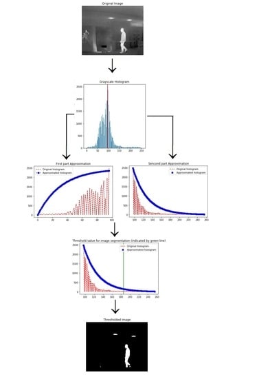
Most image thresholding methods use the grayscale histogram information of the image to find the threshold value for image segmentation. The statistical approach [31] and the functional histogram approximation approach [34] are two common approaches that are used to develop image thresholding algorithms based on the grayscale histogram information. In this section, we are describing a new functional histogram approximation-based infrared image thresholding algorithm. First, the one-dimensional histogram information such as the global maximum grayscale frequency and its corresponding intensity level are extracted to split the histogram into two parts. The reason behind extracting the global maximum and its related information is to reduce the search space region for getting an optimal threshold value for image segmentation. In the proposed method, the grayscale intensity space above the grayscale intensity corresponding to the global maximum pixel frequency was used as the search space region in order to obtain an optimal threshold value.

An image can be represented in the three-dimensional coordinate system. Let$f\left(x,y\right)$be a grayscale image where x and y represent the spatial position of the pixels and $f\left(x,y\right)$represent the intensity of the pixel located at the point $\left(x,y\right)$ on the image. The histogram of an image represents the number of pixels associated with each grayscale intensity in that image. The pixel distribution on the grayscale histogram can be represented by L discrete gray-levels, [0, 1, 2… L − 1]. The one dimensional (1D) histogram of a digital image can be defined as [35]

$$h_i=n_i; iϵ\left[0,L-1\right]$$

(1)

where $n_i$ represents the gray level frequency at gray-level$i$.

In the proposed method, the 1D-histogram of the image is partitioned into two parts based on the maximum gray-level frequency$h_m$. The first part of the histogram is represented with $h_{1i}$ and the second part of the histogram is represented with $h_{2i}$as shown in Figure 1b. The mathematical expression of the grayscale histogram of an image $h_i$can be written as

$$h_i=\{\begin{array}{c}{h}_{1i} \mathrm{for} 0\le i=f\left(x,y\right)\le i_m\\ h_{2i} \mathrm{for} i_m\le f\left(x,y\right)\le L-1\end{array}$$

(2)

here,$i_m$ is the grayscale intensity corresponding to the grayscale frequency $h_m$.

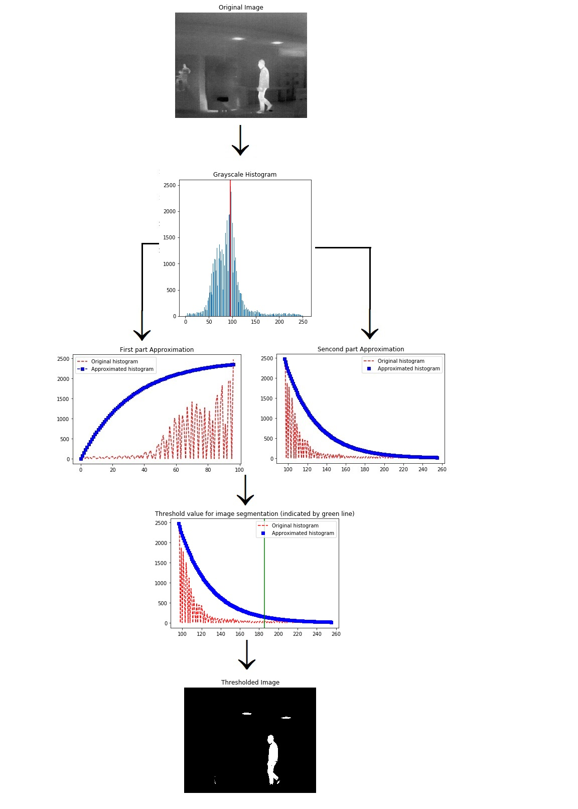
This process is explained more explicitly in Figure 1. Figure 1a shows an infrared image of the person walking and Figure 1b shows the histogram of the corresponding infrared image. In Figure 1b, we can see that the whole histogram $h_i$ is portioned into two parts based on the value of $i_m$. The first part of the histogram is labeled by $h_{1i}$ and the second part of the histogram is labeled by $h_{2i}$.

2.1. Transient Behavior of the First-Order Linear Circuit

One of the parameters used to describe the transient behavior of the first-order linear circuit is the time constant. The value of the time constant depends on the values of the circuit elements. In most cases, the circuit is designed (choosing the values for the circuit elements) based on the desired time constant value. The time at which the transient response of the circuit reaches 63% of its steady-state value is defined as the time constant. The transient response reaches 95% of its steady-state value at$3 \mathsf{\tau }$seconds and 99% of its steady-state at$5 \mathsf{\tau }$ seconds [36].

A first-order linear circuit contains one energy storing element (capacitor or inductor). Consider a first-order linear circuit connected to a step source (A) at time$t=0$. The differential equation of the circuit can be written as [37].

$$\tau \frac{dy}{dt}+y=A$$

(3)

where y is the response across the energy storing element (y is the voltage response if the storage element is a capacitor and y is the current response if the storage element is an inductor) and $\tau$represents the time-constant of the circuit.

By solving differential Equation (3), the output response of the circuit is:

$$y\left(t\right)=A\left(1-e^{-t/\tau }\right)$$

(4)

Suppose at$t=t_o$the step source is disconnected from the circuit. Now the circuit becomes a source free circuit and the differential equation for the output response can be written as

$$\tau \frac{dy}{dt}+y=0$$

(5)

By solving differential Equation (5), the output response of the circuit is:

$$y=y\left(t_o\right)e^{-\left(t-t_o\right)/\tau }$$

(6)

where $y\left(t_o\right)$is the output response at$t=t_o$ and$y\left(t_o\right)=y\left(t_o^{-}\right)=y\left(t_o^{+}\right)$.

The following is the generalized mathematical expression based on the initial value$\left(y\left(0\right)\right)$and the final value$\left(y(\infty )\right)$of the output response:

$$y=y(\infty )+\left(y\left(0\right)-y(\infty )\right)e^{-\left(t-0\right)/\tau }$$

(7)

By using Equation (7), the output response of the circuit at $t=t_1$can be expressed as

$$y=y\left(t_1\right)+\left(y\left(t_o\right)-y\left(t_1\right)\right)e^{-\left(t-t_o\right)/\tau }, t_o<t_1<\infty$$

(8)

where $y\left(t_o\right)$is the response of the circuit at the initial value $t_o$ and is equal to $A$ and $y\left(t_1\right)$is the final response of the circuit and $y\left(t_1\right)=0$as $t_1\to \infty$.

Equations (6) and (8) are used in the proposed method for approximating the grayscale histogram to the transient response of the first-order linear circuit.

2.2. Approximating the Grayscale Histogram to the Transient Response of the First-Order Linear Circuit

In the proposed method, the first part of the grayscale histogram $h_{1i}$ is approximated based on the transient response of the first-order linear circuit connected to a step source. Based on Equation (6), the mathematical expression of the approximation histogram for the first part can be written as

$${\acute{h}}_{1i}=h_m\left(1-e^{-\frac{i}{\tau }}\right)$$

(9)

where $h_m$ is the analogy of $A$ under the assumption that the steady-state value of the first part of the approximated histogram is$h_m$. Figure 2a shows the approximation histogram corresponding to the first part of the original histogram shown in Figure 1b.

Furthermore, the second part of the histogram is approximated to the transient response of the source-free first-order linear circuit. Based on Equation (8), the mathematical expression of the approximated histogram for the second part can be written as

$${\acute{h}}_{2i}=h_{L-1}+\left(h_m-h_{L-1}\right)e^{-\left(i-i_m\right)/\tau }$$

(10)

where $i_m$ is analogous to the initial time$t_o$, $h_m$ is analogous to the initial response $y\left(t_o\right)$ and $h_{L-1}$ is analogous to the final response$y\left(t_1\right)$. Figure 2b shows the approximated histogram corresponding to the second part of the original histogram shown in Figure 1b. We observe that the second part of the histogram contains grayscale frequencies of two categories such as zero grayscale frequencies and non-zero grayscale frequencies as shown in Figure 2b. For the zero grayscale frequencies category, the number of pixels associated with either background or foreground (objects) is zero. This means that no significant information exists at the grayscale values corresponding to the zero grayscale frequencies, whereas the non-zero-grayscale frequency represents the number of pixels associated with either background or foreground (objects) in the grayscale image. The second part of the approximated histogram follows the original histogram at the non-zero grayscale frequencies. As shown in Figure 2b, the approximated histogram exhibits a close resemblance to the original histogram of the infrared image at the non-zero grayscale frequencies and we can see that the resemblance was even closer at the intensity values corresponding to the foreground (object) of the infrared image, and this step of the tracing is considered as an important event in the proposed method. Based on the value of $i_m$, the approximation histogram of the image can be expressed as

$${\acute{h}}_i=\{\begin{array}{c}{\acute{h}}_{1i}, i\in \left[0,i_m\right]\\ {\acute{h}}_{2i}, i\in \left[i_m,L-1\right]\end{array}$$

(11)

2.3. Determining the Threshold Value for Image Segmentation

The thermal abnormalities in the infrared image differentiate the foreground objects from the background of the image. In general, the high-temperature regions are correlated to the foreground object and therefore the pixels belonging to the high-intensity values represent the foreground objects in the infrared imaging [38]. In the proposed method, the threshold value that separates the objects from the background can be obtained from the second part of the histogram and the threshold value is defined based on the entropy value$H$. The expression of the histogram based on the entropy is defined as

$$h_{i=T}=h_T=\left(H/100\right)\times h_m$$

(12)

By substituting Equation (12) in Equation (10), the modified expression is:

$$h_T=h_{L-1}+\left(h_m-h_{L-1}\right)e^{-\left(T-i_m\right)/\tau }$$

(13)

Simplifying Equation (13) further to get the expression for the threshold:

$$h_T-h_{L-1}=\left(h_m-h_{L-1}\right)e^{-\left(T-i_m\right)/\tau }$$

(14)

$$\frac{h_m-h_{L-1}}{h_T-h_{L-1}}=e^{\left(T-i_m\right)/\tau }$$

(15)

Applying the natural logarithm on both sides, the modified expression is:

$$\ln \left(\frac{h_m-h_{L-1}}{h_T-h_{L-1}}\right)=\frac{\left(T-i_m\right)}{\tau }$$

(16)

$$T-i_m=\tau \ln \left(\frac{h_m-h_{L-1}}{h_T-h_{L-1}}\right)$$

(17)

$$T= i_m+\tau \ln \left(\frac{h_m-h_{L-1}}{h_T-h_{L-1}}\right)$$

(18)

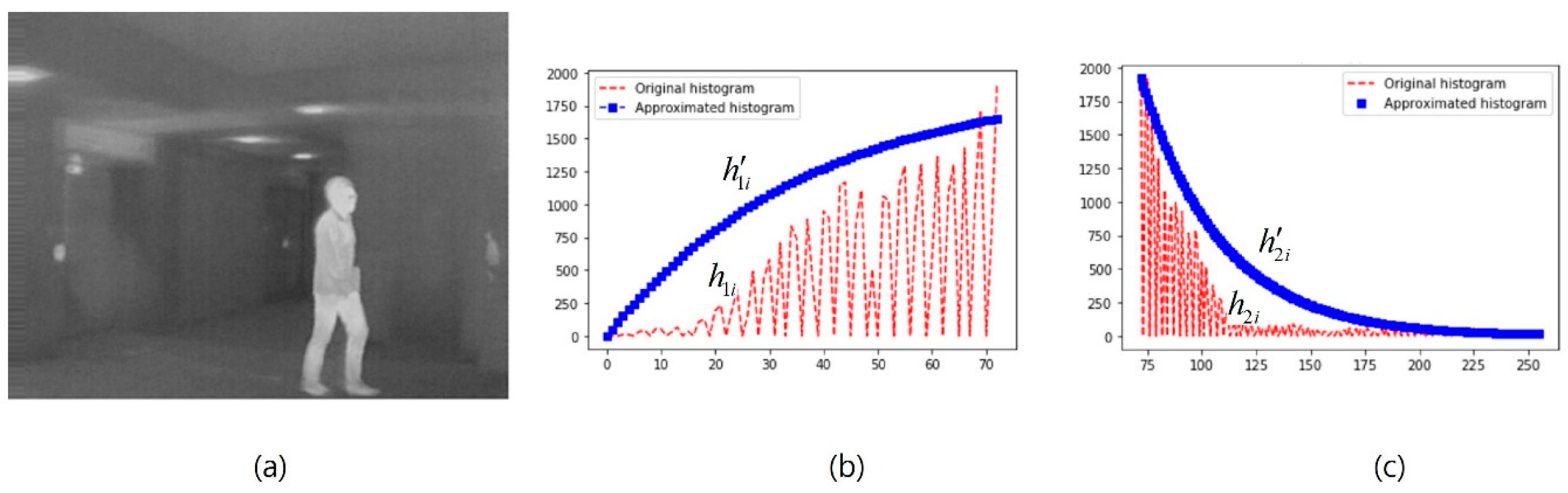
The vertical line in Figure 3 indicates the intensity threshold value obtained from the proposed method for the infrared image shown in Figure 2b.

The time-constant$\tau$is determined based on the concept of finding the approximate time taken by a linear first-order circuit to reach its steady-state. The approximate time taken by the first-order linear circuit to reach its steady-state is$5 \tau$ [36]. The procedure for finding the time-constant value is described in Figure 3. By applying this concept to the second part of the approximated histogram, we get:

$$5\tau =\left(L-1\right)-i_m$$

(19)

Simplifying further, the expression of $\tau$is:

$$\tau =\frac{\left(L-1\right)-i_m}{5}$$

(20)

In intensity thresholding, the gray-level is compared with a threshold value and based on the comparison, the grayscale image is converted into a binary image [39]. Equation (18) gives the expression of the threshold value for the image segmentation. Based on the threshold value, the image can be converted into a binary image as

$$B\left(x,y\right)=\{\begin{array}{c}0, f\left(x,y\right)<T\\ 1, f\left(x,y\right)\ge T\end{array}$$

(21)

where, $f \left(x,y\right)\le T$represents the background and$f\left(x,y\right)>T$represents the foreground of the image for an image containing light objects on a dark background.

The natural logarithmic function is defined only for positive values. In the proposed method, the natural logarithmic function defining the threshold value is not valid for the following two cases.

Case 1:

The natural logarithmic function is not defined in the proposed method for defining the threshold value when $h_m-h_{L-1}\le 0$ or $h_m\le h_{L-1}$. In this condition, the value for $h_{L-1 }$of the approximated histogram is defined as

$$h_{L-1}=0$$

(22)

Case 2:

The second case in which the natural logarithmic function defining the threshold value is not valid, when $h_T-h_{L-1}\le 0$. In this condition, the expression of the threshold value is given as

$$T=L-2$$

(23)

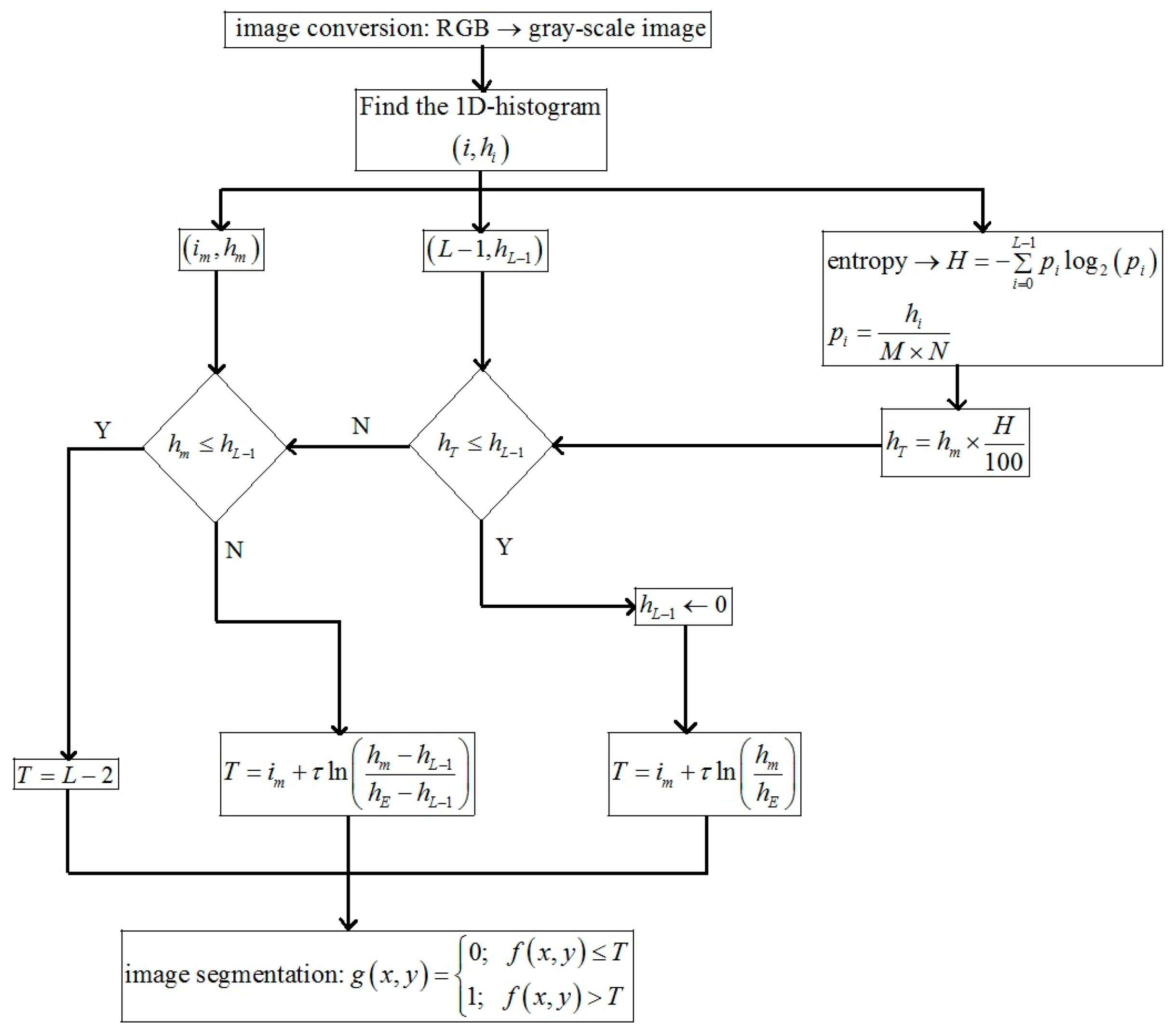
The proposed algorithm to find the threshold value for the infrared image segmentation can be explained through the flow chart as shown in Figure 4.

2.4. Validation of the Proposed Method through Approximation Error

We outlined a few things here to ensure that the proposed method was giving a precise approximated histogram to the original histogram of the infrared image. To validate the approximation, the approximation errors or relative errors$\left(e_{Approx}\right)$between the original histogram and the approximated histogram were calculated for the second part of the histogram shown in Figure 2c. The approximation error is defined as [40].

$$e_{Approx}=\left|\frac{\acute{h}\left(i\right)-h\left(i\right)}{\acute{h}\left(i\right)}\right|$$

(24)

where $h\left(i\right)$ is the grayscale frequency at the intensity level$i$ of the original histogram and $\acute{h}\left(i\right)$ is the grayscale frequency at the intensity level$i$ of the approximated histogram.

The approximation error compares the approximated histogram against the original histogram at different intensity levels. As shown in Figure 2, the second part of the histogram contains the grayscale intensities ranging from 72 to 255. To reveal the test results regarding the approximation error, we provided the values obtained for the approximation error over the duration of 6 grayscale intensities and the list of approximation errors obtained at different grayscale intensities is shown in

Table 1. List approximation errors, calculated between the original histogram and the approximated histogram for the image shown in Figure 1.

Intensity Level	Number of Pixels	Approximation Error	Intensity Level	Number of Pixels	Approximation Error
72	1918	0	168	61	0.5647
78	1271	0.2193	174	52	0.5634
102	513	0.3933	180	23	0.7728
108	279	0.611	204	61	0.1501
114	52	0.9146	210	39	0.1365
120	85	0.8357	216	40	0.0392
132	58	0.8679	222	57	0.7366
156	47	0.8740	228	41	0.4637
162	31	0.8120	234	25	0.0448

. Since the number of pixels present at the intensities corresponding to the zero grayscale frequency is zero, we omitted the approximation error calculation for these grayscale intensities. According to Table 1, the highest deviation of the approximated histogram from the original histogram is obtained at the intensity level 114. At this intensity level, the number of pixels corresponding to the original histogram is 52 however the number of pixels related to the approximated histogram using Equation (10) is 609. The lowest deviation of the approximated histogram from the original histogram is obtained at the grayscale intensity level 216. At this intensity level, the number of pixels corresponding to the original histogram is 40, however, the number of pixels related to the approximated histogram using Equation (10) is 38. The approximation error with a very low value at the grayscale intensity indicates that the grayscale frequency obtained from the approximation histogram has a value very close to the grayscale frequency of the original histogram. We observe from Table 1 that the approximation error is less than what it is for most grayscale intensities. The results of this paper finding the approximation errors imply that the approximated histogram follows the original histogram. These results further strengthened our conviction that the proposed method can generate an accurate approximation histogram to the original histogram of an infrared image. Further analyses were carried out in the next section to analyze the working performance of the proposed method by conducting experiments on infrared images collected from the standard infrared image databases.

3. Experimental Analysis and Results

We implemented the proposed method on a PC with Intel Corei7 (Intel Corporation, Santa Clara, CA, USA), 3.6 GHz processor, and 8 GB RAM. The experiments were conducted in a Python programming environment. To verify the performance of the proposed method in detecting objects using image segmentation, we tested our method on the infrared images extracted from recently developed standard databases. The original images with no modifications were considered for the experimental analysis and the database details are provided in

Table 2. List of the infrared image databases.

Dataset	Purpose	Sensor	Number of Frames	Resolution (Pixels)
LTIR	Human detection	FLIR Tau 320	358	320 × 240
	Horse detection	FLIR Photon 320	348	324 × 256
	Human detection	FLIR Photon 320	270	320 × 240
	Human detection	AIM QUIP	218	640 × 480
Photovoltaic System Thermal Images	Hotspot detection	Zenmuse XT IR camera	55	336 × 256

.

LTIR is a more challenging dataset for thermal object detection. Thermal image sequences collected in the LTIR dataset were captured with distinct image sensors in different environments and recorded on different platforms. The LTIR dataset consists of 20 sequences, in which we considered four different challenging sequences to test the proposed method. Our method was also tested on another set of infrared images in the Photovoltaic System Thermal Image Database. The purpose of selecting thermal imagery in the Photovoltaic System Thermal Image Database is to identify the hotspots caused by various faults in the photovoltaic modules. The infrared images in the Photovoltaic System Thermal Image Database are captured at different altitudes under different weather conditions.

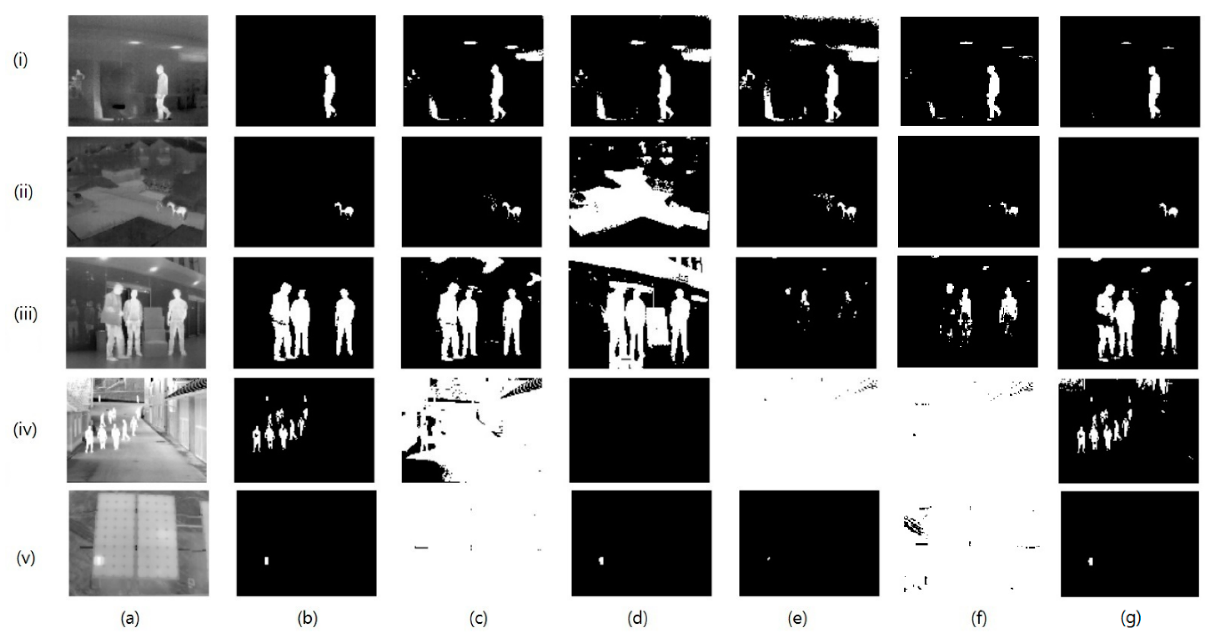
The experiments were conducted on all the images of the databases listed in Table 2. A sample image from each sequence was considered to exhibit the thresholding results of our method along with other state-of-the-art methods as shown in Figure 5. To evaluate the performance of the proposed methods, the results of our method were compared with the ground truth images shown in Figure 5b and other image thresholding methods. Figure 5c shows the thresholding results of the Yen method, Figure 5d shows the thresholding results of the Soundrapandiyan et al. method, Figure 5e shows the thresholding results of the Milad et al. method, Figure 5f shows the thresholding results of the Tao et al. method and Figure 5g shows the thresholding results of the proposed method. Although most of the results of the various methods are very close to the ground truth images, we can observe severe over-segmentation or under-segmentation in some of the results. We considered such severely over-segmented or under-segmented results to be poor performance results. The Yen method has produced poor results for Figure 5iv,v; this reveals the inconsistency of this method in the thresholding of infrared images captured under different conditions. Soundrapandiyan et al. has produced poor results for Figure 5ii,iv,v, and Milad et al. has produced poor results for Figure 5iii,iv,v. Although the two methods were developed for infrared image segmentation, the results of these methods show incompetence in thresholding infrared images, especially in the case of multi-object infrared images. Although the Tao et al. method produced satisfactory thresholding results for the first three images, this method produced over-segmented results for the next two images. It can be observed from the thresholding results that the proposed method yields consistent and satisfactory segmentation for all the images. Even though the proposed method produced better results compared to other methods, our method lags in providing more accurate results for high-resolution infrared thermal images, which we can observe in Figure 5iv,f. The proposed method is successful in thresholding single person as well as multi-person infrared thermal images, which shows the significance of our method for the purpose of person detection applications. The proposed method produced more accurate thresholding results in case of detecting hotspots in the solar PV panels, showing the effectiveness of the proposed method in real-world applications. In more detail, the performance of the proposed method was evaluated via quantitative analysis.

Quantitative Analysis

For image thresholding, the peak signal noise ratio (PSNR) [41] compares the image thresholding result of the methodology with that of the ground truth image. It reports the number of misclassified pixels of the image thresholding result of the methodology to the ground truth image:

$$\mathrm{PSNR}=20{\log }_{10}\left(L-1\right)-10{\log }_{10}\left(\frac{1}{\mathrm{M}\times \mathrm{N}}{\displaystyle \sum }_{i=0}^{M-1}{\displaystyle \sum }_{j=0}^{N-1}\left(B\left(x,y\right)-GT\left(x,y\right)\right)\right)$$

(25)

where $L$is the maximum gray level since we experimented on eight-bit images, the value of $L$ is 256; $M\times N$ is the size of the image; $B\left(x,y\right)$ is the image thresholding result and $GT\left(x,y\right)$ is the ground truth image.

Sequences named as ‘hiding’, ‘horse’, ‘mixed-distractors’, and ‘saturated’ in the LTIR dataset are the first four sequences and the image set in the Photovoltaic System Thermal Image Database is labeled as sequence 5. These five sequences are considered to evaluate the performance of the proposed method and the average peak signal noise ratio (PSNR) values obtained for each sequence are listed in

Table 3. Average peak signal noise ratio (PSNR) (in dB) results for the five methods.

Sequence	Yen Method	Soundrapandiyan et al.	Milad et al.	Tao et al.	Proposed
1	19.5227	18.9946	18.9830	21.2301	23.5662
2	28.1154	10.8097	20.7470	34.8999	35.0484
3	14.2475	14.4219	12.1629	15.0631	19.0519
4	4.7949	11.1707	19.7181	12.2039	21.1696
5	11.2230	27.4780	25.1709	17.2717	32.0171

. The performance comparison based on PSNR values obtained for the images in all sequences (total of 1249 images) is shown in Figure 6.

Sequence 1 and sequence 3 are recorded indoors to detect the human. Sequence 2 is recorded in a natural background to detect a horse. Sequence 4 offers very high-resolution images with a complex background and the purpose is to detect multi persons. Sequence 5 addresses solar energy applications where hotspots are to be detected for fault diagnosis. In order to check the detection capability through image segmentation, we considered all these sequences for evaluation. The Yen method works well for segmenting single objects in sequence 1 and sequence 2, however, this method fails to produce satisfactory single object segmentation for sequence 5. According to the PSNR metrics of the Yen method obtained for sequence 3 and sequence 4, this method is not suitable for the segmentation of multi-object infrared images. The Soundrapandiyan et al. algorithm and Milad et al. algorithm work well for single object infrared image segmentation, meanwhile, they have provided poor performance for the segmentation of multi-object infrared images related to sequence 4. The performance of Tao et al. is satisfactory for sequence 1, sequence 2, and sequence 3. However, this method produced a poor performance according to the PSNR metrics obtained for sequence 4 and sequence 5. The obtained metrics for PSNR in all sequences revealed that the proposed method can perform better segmentation for single-object infrared images and multi-object infrared images. To emphasize this fact, the finest performances were highlighted showing the best results between the comparisons.

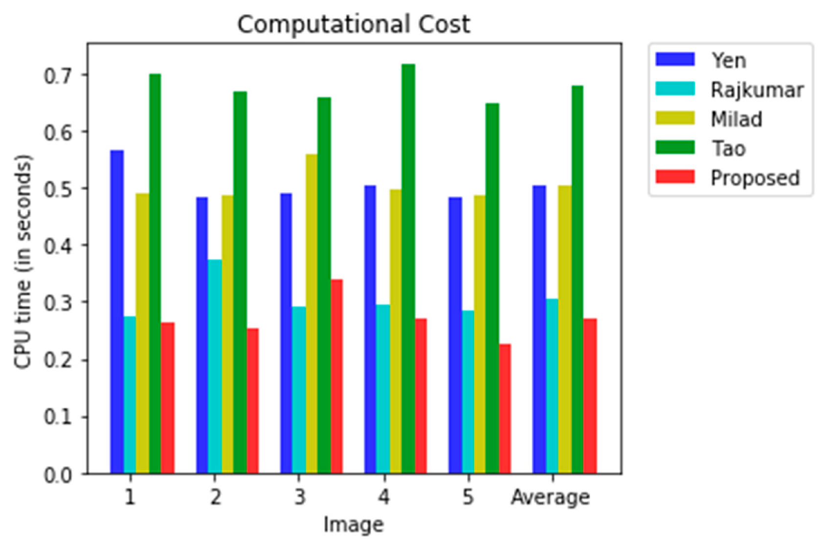
In order to assess the computational cost [42], the CPU times were measured for the images shown in Figure 5. A list of the CPU times for each method is provided in

Table 4. Computational cost (in seconds) results for the five methods.

Image	Yen Method	Soundrapandiyan et al.	Milad et al.	Tao et al.	Proposed
1	0.5660	0.2730	0.4920	0.7010	0.2630
2	0.4830	0.3750	0.4860	0.6710	0.2550
3	0.4920	0.2900	0.5590	0.6590	0.3410
4	0.5030	0.2960	0.4970	0.7180	0.2700
5	0.4850	0.2860	0.4880	0.6490	0.2250
Average	0.5038	0.3040	0.5044	0.6796	0.2708

and Figure 7. From this table, we can observe that the computational cost is high for the Yen method, Milad et al. method, and the Tao et al. method. The reason for this is the number of iterations required in these methods to generate an optimal threshold value, whereas the computational cost is less for the Soundrapandiyan et al. and the proposed method. The Soundrapandiyan et al. method requires the background subtraction of the image, which is an additional step compared to the proposed method, and this additional step causes a higher computational cost than the proposed method. The simple mathematical structure of the proposed method to produce the optimal threshold value causes the lowest computational cost of all the methods listed in Table 4.

4. Conclusions

In this paper, we found a new thresholding algorithm for infrared thermal images based on approximating the grayscale histogram of the image to the transient response of the first-order linear circuit. The simple mathematical architecture of the proposed method reduces the computational cost in searching for the optimal threshold value. Results to date have been very promising and we hope that our research will be useful in segmenting the thermal objects of the infrared images. Furthermore, our method was proven to work well for multi-object infrared thermal image thresholding. To further our research, we plan to apply our algorithm to the infrared thermal images of photovoltaic modules to detect the hotspots and try to use hotspot information to estimate the power loss caused by various faults in photovoltaic modules.

References

- Goh, T.Y.; Basah, S.N.; Yazid, H.; Aziz Safar, M.J.; Ahmad Saad, F.S. Performance analysis of image thresholding: Otsu technique. Meas. J. Int. Meas. Confed. 2018, 114, 298–307. [Google Scholar] [CrossRef]
- Chen, J.; Guan, B.; Wang, H.; Zhang, X.; Tang, Y.; Hu, W. Image Thresholding Segmentation Based on Two Dimensional Histogram Using Gray Level and Local Entropy Information. IEEE Access 2017, 6, 5269–5275. [Google Scholar] [CrossRef]
- Harb, S.M.E.; Isa, N.A.M.; Salamah, S.A. Improved image magnification algorithm based on Otsu thresholding. Comput. Electr. Eng. 2015, 46, 338–355. [Google Scholar] [CrossRef]
- Malarvel, M.; Sethumadhavan, G.; Bhagi, P.C.R.; Kar, S.; Thangavel, S. An improved version of Otsu’s method for segmentation of weld defects on X-radiography images. Optik (Stuttgart) 2017, 142, 109–118. [Google Scholar] [CrossRef]
- Yu, X.; Zhou, Z.; Gao, Q.; Li, D.; Ríha, K. Infrared image segmentation using growing immune field and clone threshold. Infrared Phys. Technol. 2018, 88, 184–193. [Google Scholar] [CrossRef]
- Zhou, D.; Zhou, H.; Shao, Y. An improved Chan-Vese model by regional fitting for infrared image segmentation. Infrared Phys. Technol. 2016, 74, 81–88. [Google Scholar] [CrossRef]
- Lin, Q.; Ou, C. Tsallis entropy and the long-range correlation in image thresholding. Signal Process. 2012, 92, 2931–2939. [Google Scholar] [CrossRef]
- Saravanan, C. Color image to grayscale image conversion. In Computer Engineering and Applications, International Conference; IEEE Computer Society: Washington, WA, USA, 2010; Volume 2, pp. 196–199. [Google Scholar] [CrossRef]
- Teutsch, M.; Mueller, T.; Huber, M.; Beyerer, J. Low resolution person detection with a moving thermal infrared camera by hot spot classification. In Proceedings of the 2014 IEEE Conference on Computer Vision and Pattern Recognition Workshops, Columbus, OH, USA, 25 September 2014; pp. 209–216. [Google Scholar] [CrossRef]
- Der, S.Z.; Chellappa, R. Probe-based automatic target recognition in infrared imagery. IEEE Trans. Image Process. 1997, 6, 92–102. [Google Scholar] [CrossRef]
- Gao, B.; Li, X.; Woo, W.L.; Tian, G.Y. Physics-based image segmentation using first order statistical properties and genetic algorithm for inductive thermography imaging. IEEE Trans. Image Process. 2018, 27, 2160–2175. [Google Scholar] [CrossRef]
- Bahramian, F.; Mojra, A. Thyroid cancer estimation using infrared thermography data. Infrared Phys. Technol. 2020, 104, 103126. [Google Scholar] [CrossRef]
- Zhou, Y.; Gao, M.; Fang, D.; Zhang, B. Tank segmentation of infrared images with complex background for the homing anti-tank missile. Infrared Phys. Technol. 2016, 77, 258–266. [Google Scholar] [CrossRef]
- Prochno, H.C.; Barussi, F.M.; Bastos, F.Z.; Weber, S.H.; Bechara, G.H.; Rehan, I.F.; Michelotto, P.V. Infrared Thermography Applied to Monitoring Musculoskeletal Adaptation to Training in Thoroughbred Race Horses. J. Equine Vet. Sci. 2020, 87, 102935. [Google Scholar] [CrossRef] [PubMed]
- Zhao, Y.; Song, Y.; Li, X.; Sulaman, M.; Guo, Z.; Yang, X.; Wang, F.; Hao, Q. IR saliency detection via a GCF-SB visual attention framework. J. Vis. Commun. Image Represent. 2020, 66. [Google Scholar] [CrossRef]
- Lu, Y.; Dong, L.; Zhang, T.; Xu, W. A robust detection algorithm for infrared maritime small and dim targets. Sensors 2020, 20, 1237. [Google Scholar] [CrossRef] [PubMed] [Green Version]
- Zhang, L.; Peng, L.; Zhang, T.; Cao, S.; Peng, Z. Infrared small target detection via non-convex rank approximation minimization joint l2,1 norm. Remote Sens. 2018, 10, 1821. [Google Scholar] [CrossRef] [Green Version]
- Mambou, S.J.; Maresova, P.; Krejcar, O.; Selamat, A.; Kuca, K. Breast cancer detection using infrared thermal imaging and a deep learning model. Sensors 2018, 18, 2799. [Google Scholar] [CrossRef] [Green Version]
- Miao, Y.; Zhu, Y.; Zhao, W.; Jiao, C.; Mo, H.; Zhang, X.; Liu, S.; Gao, H. Determination of vitamin C in foods using the iodine-turbidimetric method combined with an infrared camera. Appl. Sci. 2020, 10, 2655. [Google Scholar] [CrossRef] [Green Version]
- Akram, M.W.; Li, G.; Jin, Y.; Chen, X.; Zhu, C.; Ahmad, A. Automatic detection of photovoltaic module defects in infrared images with isolated and develop-model transfer deep learning. Sol. Energy 2020, 198, 175–186. [Google Scholar] [CrossRef]
- Du, X.; Cao, D.; Mishra, D.; Bernardes, S.; Jordan, T.R.; Madden, M. Self-adaptive gradient-based thresholding method for coal fire detection using ASTER thermal infrared data, Part I: Methodology and decadal change detection. Remote Sens. 2015, 7, 6576–6610. [Google Scholar] [CrossRef] [Green Version]
- Hristov, N.I.; Betke, M.; Kunz, T.H. Applications of thermal infrared imaging for research in aeroecology. Integr. Comp. Biol. 2008, 48, 50–59. [Google Scholar] [CrossRef] [Green Version]
- IEA-PVPS T13-10. Review on Infrared (IR) and Electroluminescence (EL) Imaging for Photovoltaic Field Applications; IEA International Energy Agency: Paris, France, 2018; ISBN 9783906042534.
- Soundrapandiyan, R.; Mouli, P.V.S.S.R.C. Adaptive Pedestrian Detection in Infrared Images Using Background Subtraction and Local Thresholding. Procedia Comput. Sci. 2015, 58, 706–713. [Google Scholar] [CrossRef] [Green Version]
- Azarbad, M.; Ebrahimzade, A.; Izadian, V. Segmentation of Infrared Images and Objectives Detection Using Maximum Entropy Method Based on the Bee Algorithm. Int. J. Comput. Inf. Syst. Ind. Manag. Appl. 2011, 3, 26–33. [Google Scholar]
- Wu, T.; Hou, R.; Chen, Y. Cloud Model-Based Method for Infrared Image Thresholding. Math. Probl. Eng. 2016, 2016, 1571795. [Google Scholar] [CrossRef] [Green Version]
- Grady, L. Random walks for image segmentation. IEEE Trans. Pattern Anal. Mach. Intell. 2006, 28, 1768–1783. [Google Scholar] [CrossRef] [PubMed] [Green Version]
- Miezianko, R.; Pokrajac, D. People detection in low resolution infrared videos. In Proceedings of the 2008 IEEE Computer Society Conference on Computer Vision and Pattern Recognition Workshops, CVPR Workshops, Anchorage, AK, USA, 1–6 July 2008. [Google Scholar] [CrossRef]
- Berg, A.; Ahlberg, J.; Felsberg, M. A thermal Object Tracking benchmark. In Proceedings of the 2015 12th IEEE International Conference on Advanced Video and Signal Based Surveillance (AVSS), Karlsruhe, Germany, 25–28 August 2015. [Google Scholar] [CrossRef] [Green Version]
- Mejia, E.A.; Correa, H.L.; Mejía, É.F.; Girón, R.; David, A.; Rodriguez, N.; Esperanza, S. Photovoltaic System Thermal Images; Mendeley Data: Amsterdam, The Netherlands, 2019. [Google Scholar] [CrossRef]
- Otsu, N. A Threshold Selection Method from Gray-Level Histograms. In IEEE Transactions on Systems, Man, and Cybernetics; IEEE: Piscataway, NJ, USA, 1979; pp. 62–66. [Google Scholar] [CrossRef] [Green Version]
- Li, C.H.; Tam, P.K.S. An iterative algorithm for minimum cross entropy thresholding. Pattern Recognit. Lett. 1998, 19, 771–776. [Google Scholar] [CrossRef]
- Yen, J.C.; Chang, F.J.; Chang, S. A New Criterion for Automatic Multilevel Thresholding. IEEE Trans. Image Process. 1995, 4, 370–378. [Google Scholar] [CrossRef] [PubMed]
- Ramesh, N.; Yoo, J.H.; Sethi, I.K. Thresholding based on histogram approximation. IEE Proc. Vis. Image Signal Process 1995, 142, 271–279. [Google Scholar] [CrossRef]
- Caballero, R.D.M.; Pineda, I.A.B.; Román, J.C.M.; Noguera, J.L.V.; Silva, J.J.C. Quadri-Histogram Equalization for infrared images using cut-off limits based on the size of each histogram. Infrared Phys. Technol. 2019, 99, 257–264. [Google Scholar] [CrossRef]
- Cahiotakis, M.; Cory, D.G. Examples of Transient RC and RL Circuits; Course Notes: Stanford, CA, USA, 2006. [Google Scholar]
- Irwin, J.D.; Nelms, R.M. Basic Engineering Circuit Analysis, 10th ed.; Wiley: Hoboken, NJ, USA, 2011; pp. 298–318. [Google Scholar]
- Berg, A. Detection and Tracking in Thermal Infrared Imagery; Linköping University Electronic Press: Linköping, Sweden, 2016; ISBN 9789176857892. [Google Scholar] [CrossRef] [Green Version]
- Umaa Mageswari, S.; Sridevi, M.; Mala, C. An experimental study and analysis of different image segmentation techniques. Procedia Eng. 2013, 64, 36–45. [Google Scholar] [CrossRef] [Green Version]
- Kreinovich, V. How to define relative approximation error of an interval estimate: A proposal. Appl. Math. Sci. 2013, 7, 211–216. [Google Scholar] [CrossRef]
- Ewees, A.A.; Abd Elaziz, M.; Al-Qaness, M.A.A.; Khalil, H.A.; Kim, S. Improved Artificial Bee Colony Using Sine-Cosine Algorithm for Multi-Level Thresholding Image Segmentation. IEEE Access 2020, 8, 26304–26315. [Google Scholar] [CrossRef]
- Wang, W.; Duan, L.; Wang, Y. Fast Image Segmentation Using Two-Dimensional Otsu Based on Estimation of Distribution Algorithm. J. Electr. Comput. Eng. 2017, 2017, 12. [Google Scholar] [CrossRef] [Green Version]
Figure 1.
(a) Infrared image of a person; (b) grayscale histogram of the image.
Figure 2.
(a) Original image; (b) the approximated part and original part for the first part of the original histogram; and (c) the approximated part and original part for the second part of the original histogram.
Figure 3.
Finding value for .
Figure 4.
Flowchart of the proposed method to find the threshold value.
Figure 5.
Comparison results of the five methods for images (i–v): (a) original image; (b) ground truth image; thresholding results: (c) Yen method; (d) Soundrapandiyan et al.; (e) Milad et al.; (f) Tao et al.; and (g) the proposed method.
Figure 6.
Comparison of the PSNR values for the five methods.
Figure 7.
Comparison of the computational cost for the five methods.