Confidence-Based Voting for the Design of Interpretable Ensembles with Fuzzy Systems †


1
Institute of Informatics and Telecommunication, Reshetnev Siberian State University of Science and Technology, Krasnoyarsk 660037, Russia
2
Department of Information Science and Technology, Aichi Prefectural University, Nakagute 480-1198, Japan
*
Author to whom correspondence should be addressed.
†
This paper is the extended version of our published in IOP Conference Series: Materials Science and Engineering, Krasnoyarsk 660037, Russia, 29 January 2020.
Algorithms 2020, 13(4), 86; https://0-doi-org.brum.beds.ac.uk/10.3390/a13040086
Submission received: 15 March 2020
/
Revised: 30 March 2020
/
Accepted: 3 April 2020
/
Published: 6 April 2020
(This article belongs to the Special Issue Mathematical Models and Their Applications)
Abstract
:In this study, a new voting procedure for combining the fuzzy logic based classifiers and other classifiers called confidence-based voting is proposed. This method combines two classifiers, namely the fuzzy classification system, and for the cases when the fuzzy system returns high confidence levels, i.e., the returned membership value is large, the fuzzy system is used to perform classification, otherwise, the second classifier is applied. As a result, most of the sample is classified by the explainable and interpretable fuzzy system, and the second, more accurate, but less interpretable classifier is applied only for the most difficult cases. To show the efficiency of the proposed approach, a set of experiments is performed on test datasets, as well as two problems of estimating the person’s emotional state with the data collected by non-contact vital sensors, which use the Doppler effect. To validate the accuracies of the proposed approach, the statistical tests were used for comparison. The obtained results demonstrate the efficiency of the proposed technique, as it allows for both improving the classification accuracy and explaining the decision making process.
1. Introduction
The development of modern classification systems in the area of computational intelligence has led to the wide application of the neural networks, decision trees and support vector machines in a variety of fields, including industry, financial sphere, medicine, engineering and social sciences. The fuzzy logic, and more precisely fuzzy classification systems, are one of the most important technologies for machine learning in cases where interpretable classifiers are required. However, every type of classification system has advantages and disadvantages; for example, the neural networks have high accuracy, but their low interpretability, while decision trees have problems with overfitting. The fuzzy systems are usually characterized by lower precision, but their advantage is that they are the “white box” classifier, i.e., their inference procedure is easily understood by experts.
The idea to combine several data mining methods together to solve the classification, regression or clustering problem is not new, and it is usually based on some implementation of voting. The advantage of voting is that it usually leads to increased generalization, so that higher accuracies are achieved on the test sets, and therefore in the real-world scenarios. For classification problems the easiest way to create an ensemble is to use the voting by majority. However, there are other ensemble design schemes, which include, but are not limited to bagging [1], boosting, [2,3,4], random forest [5], stacking [6]. The boosting algorithms include: Adaboost [7], gradient boosting [8] and random subspace method [9]. In the most efficient algorithms for ensemble generation the weighting schemes are used.
Several recent studies were focused on creating efficient schemes of generating ensembles of classifiers. In [10] the novel misclassification diversity measure as well as the incremental layered classifier selection approach were proposed. In [11] the divide-and-conuquer classifier ensemble learning algorithm is proposed, which uses many-objective problem formulation to create efficient heterogeneous ensembles. In [12] the extension of the random subspace method is proposed, called hybrid the adaptive ensemble learning. This methods introduces the new way to adapt the weights of classifiers to achieve better results with the ensemble. In [13] the novel ensemble learning algorithm is presented, which is capable of adjusting the weights of the ensemble according to current data stream. The algorithm penalizes incorrect classification and has instruments for changes detection, allowing to achieve good classification performance at every moment.
This study is focused on the development of a novel weighting technique, which uses the membership values, returned together with the class number in most fuzzy classification systems. These membership values are used as confidence levels, and the confidence-based voting decides whether the fuzzy classifier should be used, or the other, supporting classifier. This idea was originally proposed in [14]. The main difference and advantage of the proposed approach is that unlike previously mentioned methods it concentrates on combining two classifiers, where the first one is the main, and the second is the assisting classifier. This inequality of classifier roles allows receiving more interpretable and accurate results.
The experimental section contains tests on 11 problems presented at the KEEL datasets repository, as well as on data, collected by Doppler effect sensors by using non-contact vital sensing. The real-world data contained information about the person’s emotional state during listening to music.
The the paper is organized as follows: Section 2 describes the fuzzy classification method used, namely the hybrid evolutionary fuzzy classification algorithm, as well as other used classifiers applied in this study and the confidence-based voting procedure. Section 3 describes the test and real-world datasets, as well as the experimental setup and results, Section 4 contains the discussion of the results, and the conclusion is given in Section 5.
2. Materials and Methods
2.1. Classifying with Fuzzy Systems
The fuzzy logic systems originated from the fuzzy set theory, and today are applied in many areas of engineering, including data mining and machine learning. The most popular way of automated fuzzy systems design is to use evolutionary fuzzy systems (EFS) [15]. Among EFS, the fuzzy systems which are composed of a set of rules are called fuzzy rule-based systems (FRBS). The most efficient group of techniques used for FRBS design is the evolutionary algorithms, or more precisely an implementation of specific genetic algorithm (GA) [16] with modified crossover and mutation operators. These algorithms are referred to as genetic fuzzy systems (GFS) [17]. The genetic algorithms are applied because of their ability to perform search in multidimensional spaces with high efficiency. Most of the GFS algorithms try to incorporate knowledge extracted from the dataset or some kind of a priori information about the search space or problem structure. In general, the biology-inspired and evolutionary algorithms find many applications for automated design of classification and regression problems [18,19,20,21].
One of the main reasons of fuzzy systems popularity is their flexibility. Although it allows FRBS to be interpretable, there are two main directions of research: accurate fuzzy systems and interpretable fuzzy systems. The first trend is focused on generating large and complex fuzzy systems, which are usually difficult to interpret, but their accuracy is compared to the accuracy of neural networks. The second trend aims at finding relatively simple fuzzy rules, which are understandable by the experts in the subject area, but the accuracy of such systems is smaller. Their main advantage is that they are capable of extracting non-trivial knowledge available for further use. In different areas, the first or the second type of fuzzy systems are usually applied, but obviously a tradeoff between accuracy and interpretability is the main goal of most research projects.
This study uses the Hybrid Evolutionary Fuzzy Classification Algorithm (HEFCA) presented in [22]. The HEFCA algorithm have shown to be efficient for classification problems from different areas. It generates fuzzy rules, presented as follows:
where is the q-th rule, is the set of m training instances in n-dimensional space, is the fuzzy set for the i-th input variable, is the class label, and is the weight of the rule. The training set is used to normalize the sample, so that all input variables are in range [0, 1], the test set is normalized according to normalization parameters used for the training set. To calculate the resulting membership value of the rule, the product operation is used.
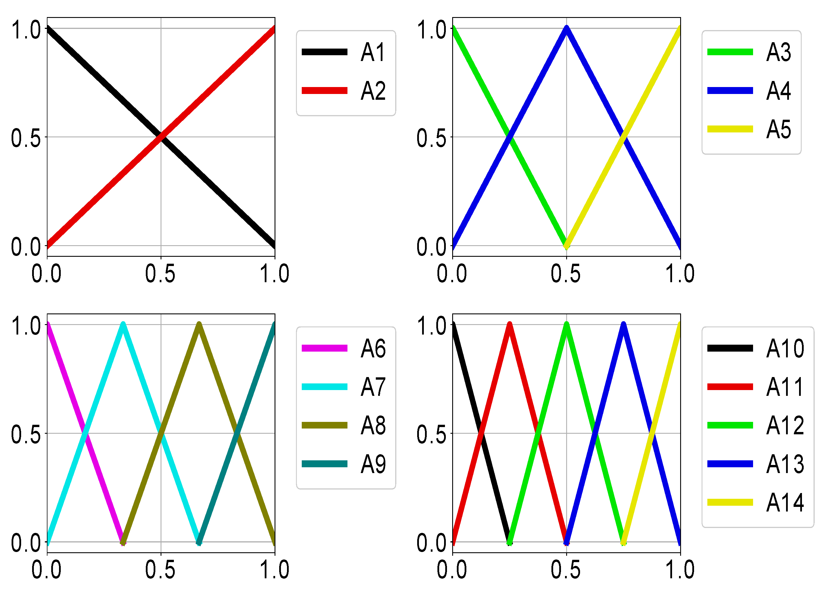
Fuzzy classifiers usually rely on a single granulation of the fuzzy variables, however this approach is not always efficient. One of the ways of improving the accuracy, proposed in [22], is to use several fuzzy granulation levels, for example into 2–5 fixed triangular terms. This allows keeping the interpretability while improving the accuracy. The used granulation is presented in Figure 1. The algorithm also used the “Don’t Care” condition to simplify the rules.
The algorithm initialized the set of rule bases using heuristic generation procedure, which uses instances from the training sample. The main loop proceeds as described in Algorithm 1:
| Algorithm 1 HEFCA main loop |
|
The quality of each generated rule was estimated using the confidence value:
where is the q-th rule left part, k is the class number, is the membership value for the value from the sample . To assign the class number to the rule, the class label having the largest confidence values is chosen. The rule weight was estimated as follows:
so that the rules which have the confidence equal to 1 receive the weight 1, and the confidence of 0.5 is mapped to zero weight. The rules having confidence lower than 0.5 are considered as empty, and if the rule base has more than 50% empty rules, it is generated again.
In this study the fitness assignment scheme was modified compared to the version of HEFCA presented in [23]. Here the loss value was added in fitness estimation, so that the fitness value is calculated as follows:
where is the total amount of misclassified points, is the number of non-empty fuzzy rules. Here is the total number of non-empty predicates in all rules, , where is the population size. Besides, N is the sample size, and is calculated as:
where w is the winner rule index. The winner rule is determined as the one which has the largest weight value. The loss value added into the fitness function makes the algorithm sensible not only to the number of misclassified instances, but also to the confidence of the classifier about its final decisions.
The Michigan part contain the following steps:
- Define each rule in a rule base as an individual and calculate its fitness;
- Remove or add new rules to the rule base with genetic or heuristic approach;
- Return the modified rule base to the population.
The Michigan-style part is applied to every rule base after the mutation operator. Firstly, the fitness values are calculated for every rule, and the rule fitness is equal to the number of correctly classified instances by this particular rule. If there are two identical rules, only one of them gets the non-zero fitness. There were three types of the Michigan part: adding new rules, deleting rules and replacing rules, i.e., first deleting, then adding. In the case of deleting rules, the number of rules k to be deleted is defined as , where S is the size of the rule base. The rules with the lowest fitness values are deleted first. In the case of adding new rules, the number of rules to be added is defined in the same way as for deleting, but if the number of rules exceeds the maximum number of rules then no rule is added.
New rules are added with the use of two different methods, heuristic and genetic ones. The heuristic method uses incorrectly classified instances to generate new rules using the same procedure as at the initialization step. The genetic method uses rules from the rule base to produce new rules with the tournament selection, uniform crossover and average mutation as in the genetic algorithm.
In addition to this the HEFCA, algorithm applied the instance selection mechanism, presented in [23]. The instance selection technique idea with balancing strategy is to generate a subsample from the original sample, where the number of instances from each label are balanced, if it is possible. This prevents the biased learning of the classifier due to existing imbalance of many datasets and also makes the search process faster, as smaller sample size is used. The probability values were assigned to each training instance, and this probability depended on the number of successful classifications of this particular instance during the adaptation period. Instances which were successfully classified many times before, are chosen less often, while complex cases are chosen with larger probabilities. The detailed procedure of instance selection is given in the HEFCA algorithm description in [23].
2.2. Classifying with Decision Trees and Neural Network Models
The development of modern data mining and machine learning tools has reached the level when the popular algorithms are implemented in various easy-to-use libraries. For example, the Keras, Tensorflow or PyTorch libaries [24] could be used for training neural networks with high computational efficiency. In this study the Keras library was used to implement two-layered neural network. The sigmoid is used as activation function, and the softmax layer was applied at the end. The loss function was implemented as cross-entropy function, and the adaptive momentum (ADAM) optimizer was applied for weights training.
The training of the network on test datasets used the following parameters: the learning rate was set to 0.003, beta1, beta2 were equal to 0.95 and 0.999 respectively, and the learning rate decay was set to 0.005. The first hidden layer contained 100 neurons, and the second hidden layer had 50 neurons. The training was performed for 25 epochs with batch size of 100. For the vital sensing datasets different architecture was used, with only one hidden layer and 20 neurons, and learning rate equal to 0.03. The presented setup is a typical usage scenario for neural networks.
In addition to the NN, the Decision Trees training implemented in sklearn library [25] were used, as well as Random Forest training. For these two algorithms, the standard training parameters were used for all cases, as this represents a typical usage scenario.
2.3. Proposed Confidence-Based Voting Approach
The neural network and the fuzzy classification method presented in previous section return some measure of confidence of the classifier together with the class number. The fuzzy rule bases generated by HEFCA are used to find the winner rule by comparing the membership values of every rule, so that the value changes in range (0,1). If this value equals one, then the classifier fully describes this instance with this rule, and if the membership is zero, than among all the rules in the base, even the winner rule has low confidence about the true class number. Furthermore, if all rules have zero confidence in their decision, then the instance is rejected, i.e., considered as misclassified. Although it is possible, the HEFCA usually generated rule bases, which described even the test sample fully.
The neural network models with softmax layer [26] also have a set of confidence values returned, which are also considered as probabilities. The values of the softmax layer are estimated as follows:
where z vector is the softmax layer input, k is the number of classes, . If the neural network is completely unaware about the class number, all are equal to , however, this situation could be only observed after initialization in most scenarios. So, the neural network does not have the rejected classification situation like fuzzy logic classifiers.
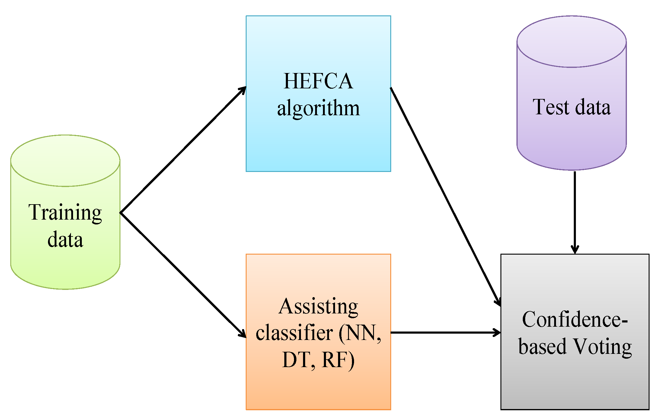
To use the fuzzy logic classifier together with other classifier, the following combination algorithm is proposed: if the membership value returned by the fuzzy logic is lower than a threshold, then the second, assisting classifier is used. That is, the main idea is to use the explainable fuzzy classifier in most cases, but apply the second, more accurate classifier, be it neural network, decision tree or random forest in more complicated cases.
The flowchart of the confidence-based voting is presented in Figure 2.
The following rule was applied in this study: after the fuzzy classifier returned the membership value and class number for all instances of the test set, of instances with lowest membership values are chosen, and a threshold value is set. These instances are classified by the assisting method. The resulting method was called the Confidence-Based Voting (CBV). The next section contains the experiments and results.
3. Results
The efficiency of the proposed CBV approach was tested on a set of databases from the KEEL repository [27]. The properties of the datasets are presented in Table 1.
The used datasets are taken from different areas, have large number of instances or classes, some of them are imbalanced, which make them difficult to solve for many machine learning methods.
The HEFCA parameters were set as follows: population size 100, number of generations 5000, maximum rule base size 40, all genetic operators, including Michigan part were self-configured. The instance selection approach used 30% of the original sample to create the training subsample, and the adaptation period was 50 generations long.
To estimate the classification quality, the 10-fold cross-validation was used. The accuracy, as well as other measures were used, including F-measure for 2-class problems, and the confusion matrix, averaged over 10 folds. The classification qualities were estimated for all classifiers separately, and then the CBV method was applied. In Table 2 the results of combining HEFCA rule bases with neural networks trained by Keras are presented.
In Table 2 the cases where the confidence-based voting led to an improvement in accuracy compared to the HEFCA results are highlighted. For seven datasets out of 11 there was an improvement observed, and for four other cases there was no improvement, because the neural network had worse results.
In Table 2, 4 and 5 in addition to the accuracies the results of the Mann–Whitney rank sum statistical test with tie-braking and normal approximation are provided. The test indicates the performance improvement (1), deterioration () or equal performance (0). Furthermore, the standard score Z-values are provided for every performed test. The p level was set to 0.05, i.e., the threshold Z values were set to and 1.96 ().
Table 3 shows the values of the F-measure for the datasets with two classes. The neural network had better values in most cases, but only for the first class, compared to the fuzzy rule bases generated by HEFCA. This is probably due to the fact that for imbalanced datasets the first class is the majority class.
Comparing the F-measures of HEFCA, NN and CBV, almost in all cases there was an improvement for the first class, except the synthetic Ring problem, where the neural network had worse results. For the second class, the F-measures were also better, compared to the results of the neural network, however these results are still worse than those of the HEFCA generated rule base.
For a better understanding of the CBV performance when combining different classifiers, the following series of experiments have been performed with Decision Tree classifier. The results are presented in Table 4.
Again, in the same way as for neural network, if the Decision Tree is better than HEFCA, then the CBV always improves the accuracy, in this case for seven datasets out of 11. Table 5 contains the results of combining HEFCA with Random Forest classifier.
The used Random Forest classifier has shown high efficiency for most of the used datasets, so that the CBV was able to improve the accuracy for 10 datasets out of 11. The only failure was for the German credit dataset, where the difference between HEFCA and RF was small, and the decrease of overall accuracy was observed, probably due to the difficulty of this classification problem.
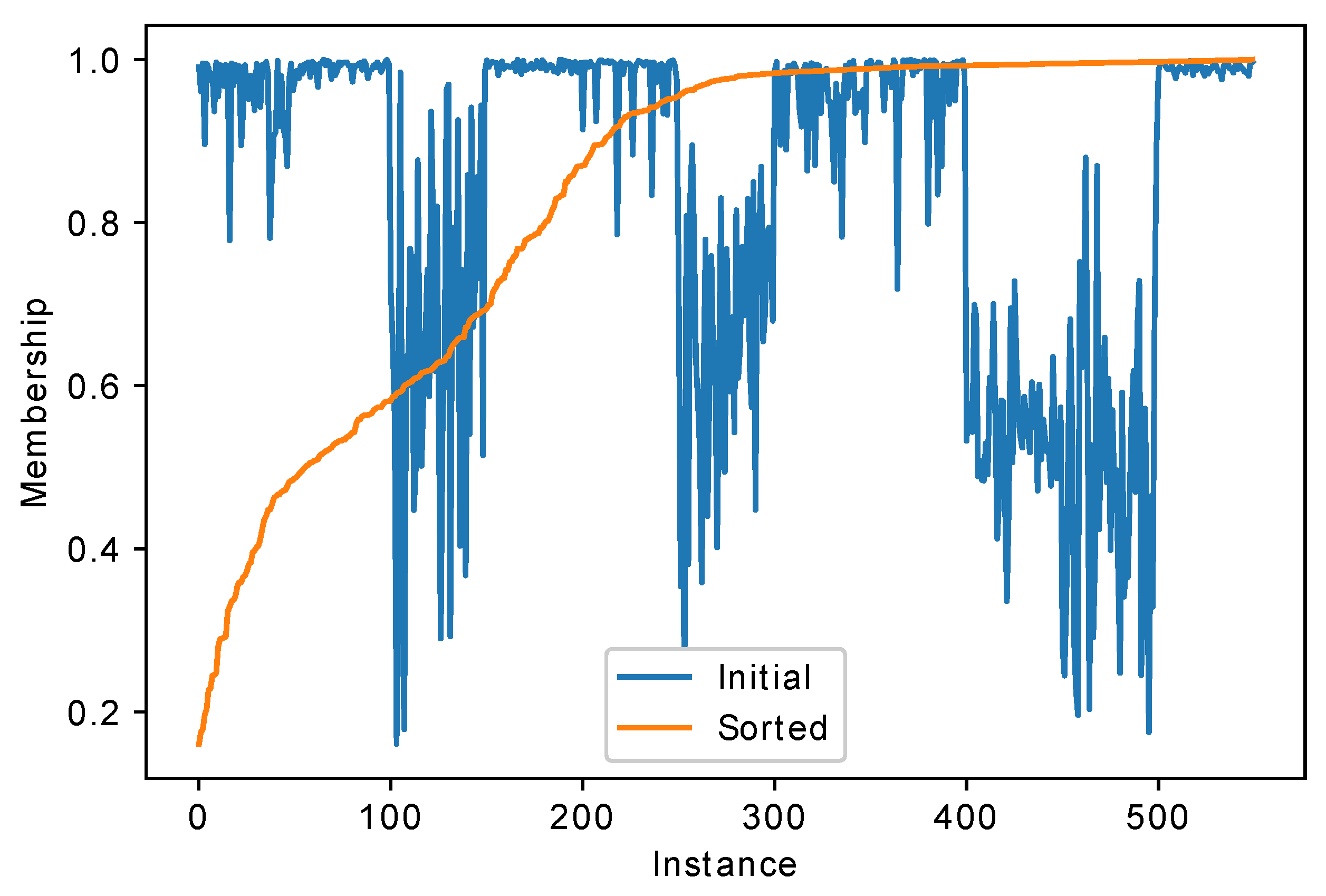
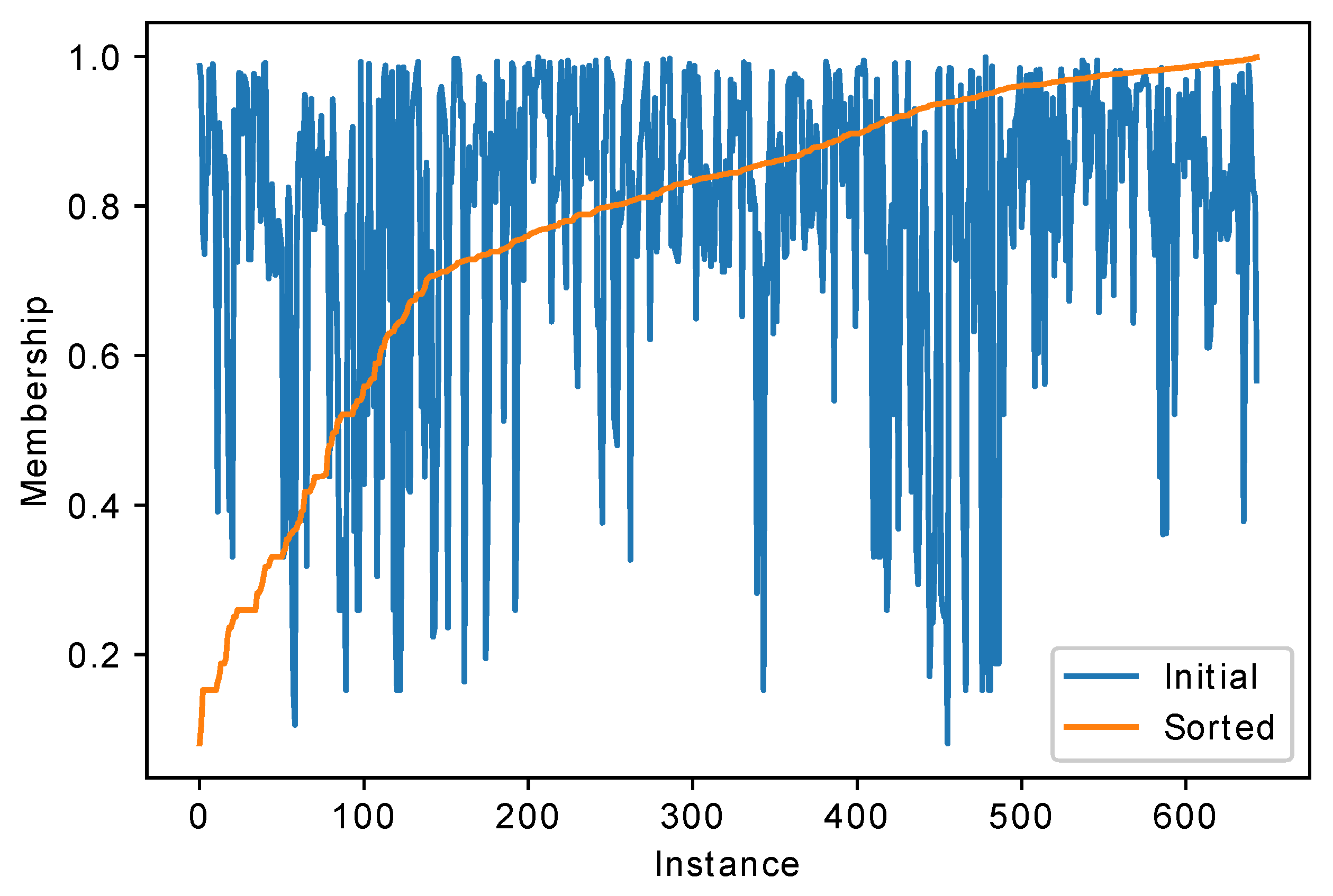
As was mentioned above, the CBV procedure was tuned so that 75% of the test set was classified by the HEFCA algorithm. For this purpose the membership values were estimated for the whole dataset, and then 25% of instances with smallest confidence were classified by other methods. Figure 3 shows the distribution of membership values returned by fuzzy classifier for the Texture problem, on one of the folds.
The texture dataset was sorted by class numbers. From Figure 3 it could be seen that the HEFCA classifier is relatively confident about most classes, but has low confidence in other classes. For example, the first two classes, around 100 instances, have membership values mostly larger then 0.9, while for the third class the membership values drop down to 0.7 or even lower. This happens due to the fuzzy rule base structure: there are rules which describe some classes very well, but other classes are poorly recognized.
Furthermore, the sorted membership values graph shows that around half of the dataset is classified with very high confidence close to 1, but for the rest of the dataset the HEFCA classifier has low confidence in its decisions.
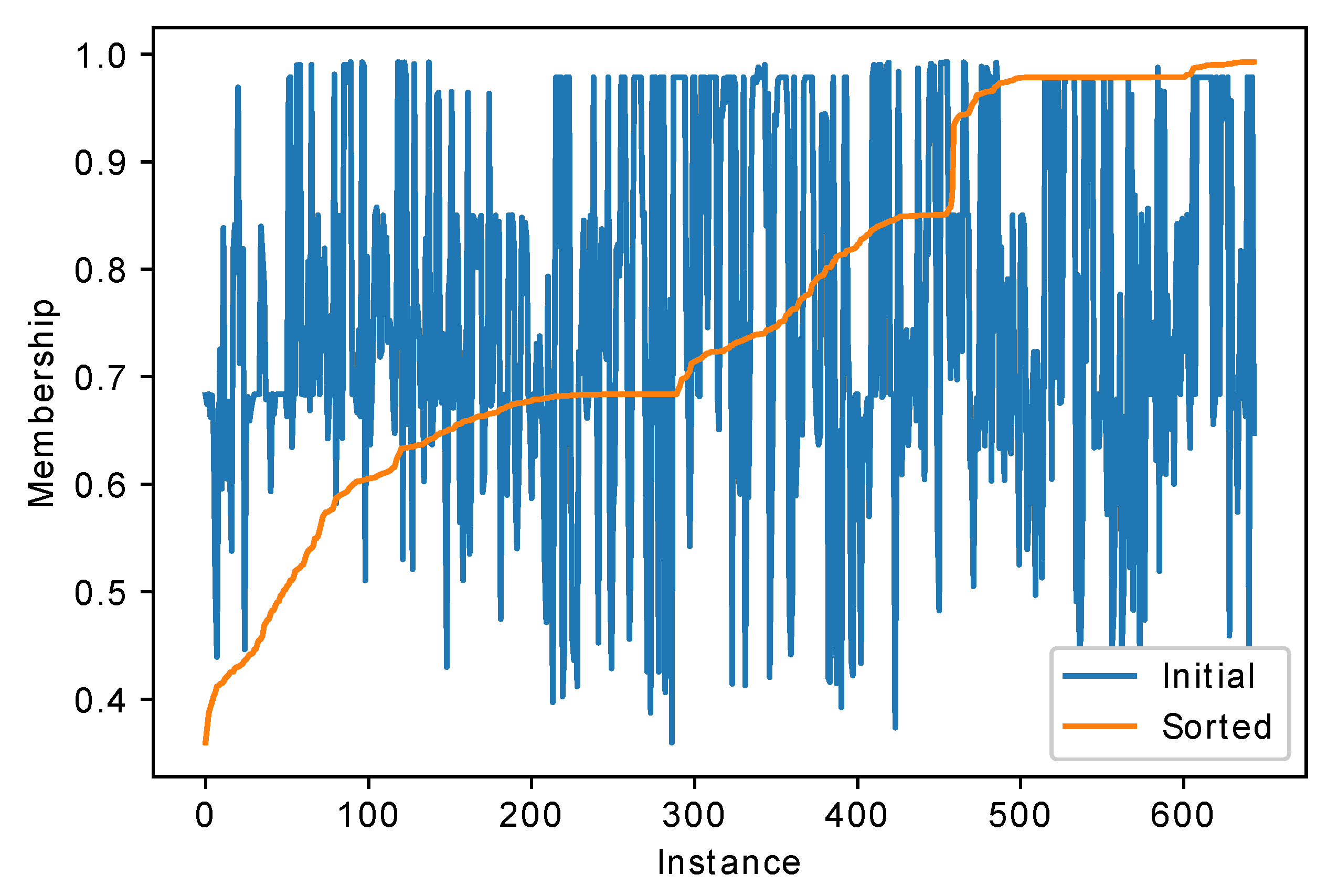
For some other classifiers, for example neural net, one may also estimate the confidence of the classifier in the class number. For example, the probabilities returned by the softmax layer of the neural net for the same texture dataset are presented in Figure 4.
Compared to the fuzzy classifier, the neural net has larger confidences; however, this does not mean that the accuracy will be larger. Here it could be seen that sometimes in cases when the fuzzy classifier has small confidence, the neural network is relatively confident, and vice versa, for example, for the last class.
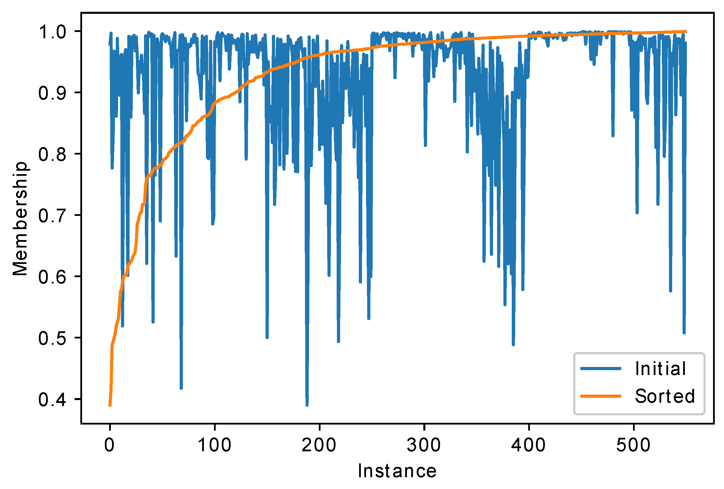
Figure 5 and Figure 6 present the confidences graphs of HEFCA and NN trained in Keras for the satimage dataset.
From Figure 5 it could be seen that for around 80% of the test sample the confidence of the HEFCA algorithm is larger than 0.75, for other instances the membership values drop. The accuracy for this dataset is around 0.87, and 85% of the test set has confidence larger than 0.5. For the neural network, the confidence changes differently, i.e., only a small part of the dataset is classified with high confidence.
In Figure 7 the influence of threshold value on the CBV accuracy for different datasets is presented.
The threshold values were changed from 0.05 to 0.5 with 0.05 step. As could be seen from Figure 7, for most datasets where the random forest had better results than HEFCA, the accuracy grows with larger threshold, i.e., with larger percentage of the test sample classified by random forest. However, for some datasets, for example, twonorm or german credit, there is almost no accuracy increase, probably due to the fact that the fuzzy classifier and random forest make errors on the same instances.
The testing of CBV efficiency on the real-world data were performed with using the information gained from the set of measurements performed by vital sensors, which used the Doppler Effect [28]. The goal of these measurements was to estimate the person’s emotional reaction when listening to different types of music. For this purpose, ten people having different gender and age were asked to be measured, and three states were set for the experiment:
- Listening to music that a participant liked during three time periods;
- Listening to music that a participant disliked during three time periods;
- Not listening to music at all during two time periods.
The processing of the raw signal from Doppler sensors was performed with the ARS technique described in [29]. In accordance with number of performed experiments, eight instances were received from the raw data, with four attributes, characterizing the respiratory rate parameters.
The resulting dataset was normalized, and according to the goal of the experiments two separate problems were formulated, with properties presented in Table 6.
- The “Listened” problem, in which an instance was labelled as “1”, listened to music, and “0” otherwise;
- The “Liked” problem, in which an instance was labelled as “1”, liked the music, and “0” otherwise.
The parameters of the HEFCA algorithm were changed to match the properties of the collected dataset, in particular the number of generations was set to 500. The neural network architecture was changed, i.e., it had only 20 nodes in a single hidden layer, and the number of epochs for training was set to 5. Same as for the test datasets, accuracy, F-measure and confusion matrix were estimated. The results of the experiments are presented in Table 7 and Table 8.
For the first problem “Liked” the CBV did not deliver any accuracy improvements, probably due to the fact that the accuracy is too low. This could happen because of the small size of the available training set. The second problem, “Listened”, was classified better, i.e., the neural network had much better accuracy, but the F-measure was equal to 0, which shows that the neural network actually did not recognize one of the classes, while the HEFCA generated classifier did it. The combination of these methods with CBV resulted in increased F-measure values for the second class, but the F-measure on the first class has dropped.
In the next two Table 9 and Table 10, the confusion matrixes are presented for both “Liked” and “Listened” problems.
The confidence-based voting procedure has allowed improving the quality of classification, in particular, the second class was recognized much better. For the “Listened” problem, the accuracy was also improved for the second class, the reason for this is that the neural network classified all instances to the second class. Still, with CBV the accuracy of the fuzzy classifier was improved.
4. Discussion
The Confidence-Based Voting procedure realizes relatively simple idea of combining two classifiers: if one of the classifiers is not sure in its final decision, then the other classifier may help make the right decision. The experiments on several datasets have shown that this idea works relatively good in many scenarios for classifiers which have some kind of confidence measure. For example, the HEFCA algorithm used in this study has clear measure of confidence, i.e., the membership value returned by the winner rule, however other classifiers, like neural network with softmax layer, could be used as well. For other classifiers, these confidence measures could be constructed, for example, for the k-NN classifier this could be the fraction of neighbors belonging to the right class, or the relative size of the final leaf in case of decision tree, or the ratio of the number of trees voting for the same class in random forest. So, the CBV is a relatively simple and efficient technique, which could be expanded also for more than 2 classifiers.
Unlike many other studies, which are concerned about accuracy of the designed classifier, in this study, the interpretability of the resulting classification system was one of the main goals. That is, with Confidence-Based Voting, we get a well-explained classification of every instance from the test set, and with relatively large membership value. Most fuzzy classifiers return membership values together with class numbers, and in real-world scenarios where interpretability is important, only those fuzzy rules which work with high membership values represent particular interest for the researchers, if they contain non-trivial dependencies. With CBV, it is possible, for example, to combine several fuzzy classifiers with different structure and different decision making procedure, so that different explanations are given for different parts of the dataset. So, unlike many ensemble methods, which simply assign weights to classifiers, the CBV is a white box, i.e., explainable procedure of decision making, which is an important property for real-world problems.
5. Conclusions
This paper propose the novel voting procedure to use with two classifiers, called the confidence-based voting. The main role in the CBV is played by the fuzzy logic based classifier, generated by HEFCA algorithm. As an assisting basic learning, any other classifier could be used: in this study the neural net, decision tree and random forest were used. The classifiers are capable of improving each other’s results thanks to the different properties: the fuzzy rule base is capable of generating interpretable rule bases, while other classifiers are usually more accurate. The CBV filters the most complicated cases where the fuzzy system is not sure, and applies the assisting classifier. The decision on which classifier to use is controlled by the threshold value, which in this study was defined based on test sample classification confidences. For the test problems, as well as real-world ones, the CBV allowed to achieve better accuracies, as well as F-measures, but only in cases when the assisting classifier was better than the fuzzy rule base. The proposed algorithm is a general scheme for combining two or more classifiers, so that not only fuzzy logic, neural networks, decision trees and random forest could be applied. Further studies may include experimenting with different basic learners, combination of other fuzzy logic based methods, or introducing voting of several classifiers with same confidence measures.
Author Contributions
Conceptualization, V.S. and S.A.; methodology, V.S., S.A. and Y.K.; software, V.S. and Y.K.; validation, V.S., S.A. and Y.K.; formal analysis, S.A.; investigation, V.S.; resources, Y.K. and V.S.; data curation, Y.K.; writing–original draft preparation, V.S. and S.A.; writing–review and editing, V.S.; visualization, S.A. and V.S.; supervision, Y.K.; project administration, Y.K. and S.A.; funding acquisition, S.A. and V.S. All authors have read and agreed to the published version of the manuscript.
Funding
This research was funded by the Council for grants of the President of the Russian Federation for young researchers, grant number MK-1579.2020.9 in 2020-2022.
Conflicts of Interest
The authors declare no conflict of interest.
Abbreviations
The following abbreviations are used in this manuscript:
| EA | Evolutionary Algorithm |
| FL | Fuzzy Logic |
| HEFCA | Hybrid Evolutionary Fuzzy Classification Algorithm |
| NN | Neural Network |
| CBV | Confidence-Based Voting |
References
- Breiman, L. Bagging predictors. Mach. Learn. 1996, 24, 123–140. [Google Scholar] [CrossRef] [Green Version]
- Freund, Y. 1997 A decision-theoretic generalization of on-line learning and an application to boosting. J. Comput. Syst. Sci. 1997, 55, 119–139. [Google Scholar] [CrossRef] [Green Version]
- Quinlan, J.R. Bagging, boosting, and C4.5. AAAI/IAAI 1996, 1, 725–730. [Google Scholar]
- Kearns, M.J. Thoughts on hypothesis boosting. 1988, pp. 319–320. Available online: https://www.semanticscholar.org/paper/Thoughts-on-hypothesis-boosting-Kearns/8688397debc570d14e0a5b5ebe53ded69feeae7b (accessed on 4 April 2020).
- Breiman, L. Random forests. Mach. Learn. 2001, 45, 5–32. [Google Scholar] [CrossRef] [Green Version]
- Wolpert, D.H. Stacked generalization. Neural Netw. 1992, 5, 241–259. [Google Scholar] [CrossRef]
- Schapire, R.E. The boosting approach to machine learning: An overview. In Nonlinear Estimation and Classification; Springer: New York, NY, USA, 2003; Volume 24, pp. 149–171. [Google Scholar]
- Friedman, J.H. Greedy function approximation: A gradient boosting machine. Annals Stat. 2001, 1189–1232. [Google Scholar] [CrossRef]
- Skurichina, M.; Duin, R.P.W. Bagging, boosting and the random subspace method for linear classifiers. Pattern Anal. Appl. 2002, 5, 121–135. [Google Scholar] [CrossRef]
- Jan, M.Z.; Verma, B. A Novel Diversity Measure and Classifier Selection Approach for Generating Ensemble Classifiers. IEEE Access 2019, 7, 156360–156373. [Google Scholar] [CrossRef]
- Asafuddoula, M.; Verma, B.; Zhang, M. A Divide-and-Conquer-Based Ensemble Classifier Learning by Means of Many-Objective Optimization. IEEE Trans. Evolut. Comput. 2018, 22, 762–777. [Google Scholar] [CrossRef]
- Yu, Z.; Li, L.; Liu, J.; Han, G. Hybrid Adaptive Classifier Ensemble. IEEE Trans. Cybern. 2015, 45, 177–190. [Google Scholar]
- Pratama, M.; Pedrycz, W.; Lughofer, E. Evolving Ensemble Fuzzy Classifier. IEEE Trans. Fuzzy Syst. 2018, 26, 2552–2567. [Google Scholar] [CrossRef] [Green Version]
- Stanovov, V.; Akhmedova, S.; Kamiya, Y. Confidence-based voting procedure for combining fuzzy systems and neural networks. IOP Conf. Ser. Mater. Sci. Eng. 2020, 24, 734:012087. [Google Scholar] [CrossRef]
- Fazzolari, M.; Alcala, R.; Nojima, Y.; Ishibuchi, H.; Herrera, F. A review of the application of multiobjective evolutionary fuzzy systems: Current status and further directions. IEEE Trans. Fuzzy Syst. 2013, 21, 45–65. [Google Scholar] [CrossRef]
- Holland, J.H. Adaptation in Natural and Artificial Systems: An Introductory Analysis with Applications to Biology, Control, and Artificial Intelligence; MIT Press: Cambridge, MA, USA, 1992. [Google Scholar]
- Herrera, F. Genetic fuzzy systems: Taxonomy, current research trends and prospects. Evol. Intell. 2008, 1, 27–46. [Google Scholar] [CrossRef]
- Zhang, Z.-C.; Hong, W.-C.; Li, J. Electric load forecasting by hybrid self-recurrent support vector regression model with variational mode decomposition and improved cuckoo search algorithm. IEEE Access 2020, 8, 14642–14658. [Google Scholar] [CrossRef]
- Zhang, Z.-C.; Hong, W.-C. Electric load forecasting by complete ensemble empirical model decomposition adaptive noise and support vector regression with quantum-based dragonfly algorithm. Nonlinear Dynam. 2019, 98, 1107–1136. [Google Scholar] [CrossRef]
- Dong, Y.; Zhang, Z.; Hong, W.-C. A hybrid seasonal mechanism with a chaotic cuckoo search algorithm with a support vector regression model for electric load forecasting. Energies 2018, 11, 1009. [Google Scholar] [CrossRef] [Green Version]
- Kundra, H.; Sadawarti, H. Hybrid algorithm of cuckoo search and particle swarm optimization for natural terrain feature extraction. Res. J. Inf. Technol. 2015, 7, 58–69. [Google Scholar] [CrossRef] [Green Version]
- Stanovov, V.; Semenkin, E.; Semenkina, O. Self-configuring hybrid evolutionary algorithm for fuzzy classification with active learning. IEEE Congr. Evolut. Comput. 2015, 1823–1830. [Google Scholar]
- Stanovov, V.; Semenkin, E.; Semenkina, O. Self-configuring hybrid evolutionary algorithm for fuzzy imbalanced classification with adaptive instance selection. J. Artif. Intell. Soft Comput. Res. 2016, 6, 173–188. [Google Scholar] [CrossRef] [Green Version]
- Chollet, François and Others, Keras. 2015. Available online: https://keras.io (accessed on 6 April 2020).
- Pedregosa, F.; Varoquaux, G.; Gramfort, A.; Michel, V.; Thirion, B.; Grisel, O.; Blondel, M.; Prettenhofer, P.; Weiss, R.; Dubourg, V.; et al. Scikit-learn: Machine Learning in Python. J. Mach. Learn. Res. 2011, 12, 2825–2830. [Google Scholar]
- Goodfellow, I.; Bengio, Y.; Courville, A. Deep Learning; MIT Press: Cambridge, MA, USA, 2016; 800p, Available online: http://www.deeplearningbook.org (accessed on 6 April 2020).
- Alcalá-Fdez, J.; Sánchez, L.; Garcia, S.; del Jesus, M.J.; Ventura, S.; Garrell, J.M.; Otero, J.; Romero, C.; Bacardit, J.; Rivas, V.M.; et al. KEEL: A software tool to assess evolutionary algorithms for data mining problems. Soft Comput. 2009, 13, 307–318. [Google Scholar] [CrossRef]
- Kamiya, Y. A new simple preprocessing method for MUSIC suitable for non-contact vital sensing using Doppler sensors. In Proceedings of the Intelligent Interactive Multimedia Systems and Services (IIMSS 2017), Vilamoura, Protugal, 21–23 June 2017; pp. 514–524. [Google Scholar]
- Kamiya, Y. A simple parameter estimation method for periodic signals applicable to vital sensing using Doppler sensors. J. Contr. Meas. Syst. Integr. 2017, 10, 378–384. [Google Scholar] [CrossRef] [Green Version]
Figure 1.
Fuzzy granulation into 2, 3, 4 and 5 terms.

Figure 2.
Flowchart of the Confidence-Based Voting.

Figure 3.
Fuzzy membership values returned by HEFCA algorithm, texture dataset, test set.

Figure 4.
Neural net outputs returned from softmax layer for the true class, texture dataset, test set.
Figure 4.
Neural net outputs returned from softmax layer for the true class, texture dataset, test set.

Figure 5.
Fuzzy membership values returned by HEFCA algorithm, satimage dataset, test set.

Figure 6.
Neural net outputs returned from softmax layer for the true class, satimage dataset, test set.
Figure 6.
Neural net outputs returned from softmax layer for the true class, satimage dataset, test set.

Figure 7.
CBV accuracy dependence on the threshold value, random forest as assisting classifier.


Table 1.
Datasets used in the experiments.
| Dataset | Number of Instances | Number of Features | Number of Classes |
|---|---|---|---|
| Australian credit | 690 | 14 | 2 |
| German credit | 1000 | 24 | 2 |
| Magic | 19,020 | 10 | 2 |
| Page-blocks | 5472 | 10 | 5 |
| Penbased | 10,992 | 16 | 10 |
| Phoneme | 5404 | 5 | 2 |
| Ring | 7400 | 20 | 2 |
| Satimage | 6435 | 36 | 6 |
| Segment | 2310 | 19 | 7 |
| Texture | 5500 | 40 | 11 |
| Twonorm | 7400 | 20 | 2 |
Table 2.
Accuracy of HEFCA, neural network and CBV.
| Dataset | HEFCA | NN (Keras) | CBV | MW Test | Z Value |
|---|---|---|---|---|---|
| Australian credit | 0.8537 | 0.8695 | 0.8551 | 0 | −0.60 |
| German credit | 0.7280 | 0.7610 | 0.7310 | 0 | 2.66 |
| Magic | 0.8415 | 0.8284 | 0.8362 | −1 | −2.49 |
| Page-blocks | 0.9406 | 0.9589 | 0.9461 | 0 | 0.75 |
| Penbased | 0.9395 | 0.9874 | 0.9790 | 1 | 3.77 |
| Phoneme | 0.8260 | 0.7972 | 0.8225 | 0 | −0.75 |
| Ring | 0.9236 | 0.8259 | 0.9008 | −1 | −3.25 |
| Satimage | 0.8636 | 0.7640 | 0.8244 | −1 | −3.77 |
| Segment | 0.9100 | 0.9498 | 0.9429 | 1 | 3.33 |
| Texture | 0.9122 | 0.9653 | 0.9356 | 1 | 2.64 |
| Twonorm | 0.9043 | 0.9805 | 0.9305 | 1 | 3.56 |
Table 3.
F-measures of HEFCA, neural network and CBV.
| Dataset | HEFCA | NN (Keras) | CBV | |||
|---|---|---|---|---|---|---|
| Class 1 | Class 2 | Class 1 | Class 2 | Class 1 | Class 2 | |
| Australian credit | 0.567 | 0.686 | 0.585 | 0.680 | 0.571 | 0.684 |
| German credit | 0.793 | 0.304 | 0.811 | 0.247 | 0.800 | 0.272 |
| Magic | 0.773 | 0.430 | 0.776 | 0.404 | 0.777 | 0.409 |
| Phoneme | 0.802 | 0.394 | 0.808 | 0.334 | 0.805 | 0.379 |
| Ring | 0.645 | 0.653 | 0.614 | 0.631 | 0.636 | 0.649 |
| Twonorm | 0.646 | 0.642 | 0.663 | 0.662 | 0.652 | 0.649 |
Table 4.
Accuracy of HEFCA, Decision Tree and CBV.
| Dataset | HEFCA | Decision Tree | CBV | MW Test | Z Value |
|---|---|---|---|---|---|
| Australian credit | 0.8537 | 0.8158 | 0.8493 | 0 | −0.30 |
| German credit | 0.728 | 0.697 | 0.723 | 0 | −0.15 |
| Magic | 0.8415 | 0.8162 | 0.8359 | 0 | −1.43 |
| Page-blocks | 0.9406 | 0.9627 | 0.9475 | 0 | 1.58 |
| Penbased | 0.9395 | 0.9616 | 0.9646 | 1 | 3.77 |
| Phoneme | 0.826 | 0.8701 | 0.8481 | 1 | 2.79 |
| Ring | 0.9237 | 0.8785 | 0.9101 | −1 | −2.78 |
| Satimage | 0.8636 | 0.8609 | 0.8712 | 0 | 1.21 |
| Segment | 0.91 | 0.9654 | 0.9537 | 1 | 3.92 |
| Texture | 0.9122 | 0.9298 | 0.9235 | 0 | 1.43 |
| Twonorm | 0.9043 | 0.847 | 0.8907 | −1 | −3.02 |
Table 5.
Accuracy of HEFCA, Random Forest and CBV.
| Dataset | HEFCA | Random Forest | CBV | MW Test | Z Value |
|---|---|---|---|---|---|
| Australian credit | 0.8537 | 0.8594 | 0.8551 | 0 | −0.30 |
| German credit | 0.728 | 0.731 | 0.72 | 0 | 0.23 |
| Magic | 0.8415 | 0.8662 | 0.8533 | 1 | 3.02 |
| Page-blocks | 0.9406 | 0.9704 | 0.9507 | 1 | 2.04 |
| Penbased | 0.9395 | 0.9871 | 0.9783 | 1 | 3.77 |
| Phoneme | 0.826 | 0.9034 | 0.8593 | 1 | 3.40 |
| Ring | 0.9237 | 0.9359 | 0.9299 | 0 | 1.43 |
| Satimage | 0.8636 | 0.9038 | 0.8921 | 1 | 3.77 |
| Segment | 0.91 | 0.9797 | 0.961 | 1 | 3.79 |
| Texture | 0.9122 | 0.9696 | 0.9349 | 1 | 3.10 |
| Twonorm | 0.9043 | 0.9477 | 0.9188 | 1 | 2.42 |
Table 6.
Datasets generated from the vital sensing experiments.
| Problem | Classes | Dataset Sizes |
|---|---|---|
| “Listened” | 1 – listened to music | 1: 20 instances |
| 2 – did not listen to music | 2: 60 instances | |
| whole set: 80 instances | ||
| “Liked” | 1 – liked music | 1: 30 instances |
| 2 – did not like music | 2: 30 instances | |
| whole set: 60 instances |
Table 7.
Accuracies of HEFCA, neural network and CBV on real-world problems.
| Dataset | HEFCA | NN (Keras) | CBV |
|---|---|---|---|
| Liked | 0.616 | 0.550 | 0.600 |
| Listened | 0.613 | 0.750 | 0.688 |
Table 8.
F-measures of HEFCA, neural network and CBV on real-world problems.
| Dataset | HEFCA | NN (Keras) | CBV | |||
|---|---|---|---|---|---|---|
| Class 1 | Class 2 | Class 1 | Class 2 | Class 1 | Class 2 | |
| Liked | 0.535 | 0.465 | 0.419 | 0.482 | 0.539 | 0.482 |
| Listened | 0.220 | 0.784 | 0.000 | 0.857 | 0.155 | 0.823 |
Table 9.
Confusion matrixes for the “Liked” problem.
| HEFCA | Actual | ||
| Predicted | Class 1 | Class 2 | Reject |
| 2.1 | 0.9 | 0 | |
| 1.4 | 1.6 | 0 | |
| NN (Keras) | Actual | ||
| Predicted | Class 1 | Class 2 | Reject |
| 1.6 | 1.4 | 0 | |
| 1.3 | 1.7 | 0 | |
| CBV | Actual | ||
| Predicted | Class 1 | Class 2 | Reject |
| 1.9 | 1.1 | 0 | |
| 1.3 | 1.7 | 0 | |
Table 10.
Confusion matrixes for the “Listened” problem.
| HEFCA | Actual | ||
| Predicted | Class 1 | Class 2 | Reject |
| 1.0 | 1.0 | 0 | |
| 2.1 | 3.9 | 0 | |
| NN (Keras) | Actual | ||
| Predicted | Class 1 | Class 2 | Reject |
| 0.0 | 2.0 | 0 | |
| 0.0 | 6.0 | 0 | |
| CBV | Actual | ||
| Predicted | Class 1 | Class 2 | Reject |
| 0.7 | 1.3 | 0 | |
| 1.2 | 4.8 | 0 | |
© 2020 by the authors. Licensee MDPI, Basel, Switzerland. This article is an open access article distributed under the terms and conditions of the Creative Commons Attribution (CC BY) license (http://creativecommons.org/licenses/by/4.0/).
Share and Cite
MDPI and ACS Style
Stanovov, V.; Akhmedova, S.; Kamiya, Y. Confidence-Based Voting for the Design of Interpretable Ensembles with Fuzzy Systems. Algorithms 2020, 13, 86. https://0-doi-org.brum.beds.ac.uk/10.3390/a13040086
AMA Style
Stanovov V, Akhmedova S, Kamiya Y. Confidence-Based Voting for the Design of Interpretable Ensembles with Fuzzy Systems. Algorithms. 2020; 13(4):86. https://0-doi-org.brum.beds.ac.uk/10.3390/a13040086
Chicago/Turabian StyleStanovov, Vladimir, Shakhnaz Akhmedova, and Yukihiro Kamiya. 2020. "Confidence-Based Voting for the Design of Interpretable Ensembles with Fuzzy Systems" Algorithms 13, no. 4: 86. https://0-doi-org.brum.beds.ac.uk/10.3390/a13040086
Note that from the first issue of 2016, this journal uses article numbers instead of page numbers. See further details here.