Short-Term Wind Speed Forecasting Using Statistical and Machine Learning Methods


1
Department of Statistics, University of Venda Private Bag X5050, Thohoyandou 0950, South Africa
2
DST-CSIR National e-Science Postgraduate Teaching and Training Platform (NEPTTP), LG07, Mathematical Sciences Building, West Campus, Private Bag 3, Wits 2050, Gauteng, South Africa
3
Department of Computer Science and Information Technology, Sol Plaatje University, Kimberley 8300, South Africa
4
Department of Statistics, University of Witwatersrand, Private Bag 3, Wits 2050, Gauteng, South Africa
*
Author to whom correspondence should be addressed.
†
These authors contributed equally to this work.
Algorithms 2020, 13(6), 132; https://0-doi-org.brum.beds.ac.uk/10.3390/a13060132
Submission received: 23 March 2020
/
Revised: 17 May 2020
/
Accepted: 19 May 2020
/
Published: 26 May 2020
Abstract
:Wind offers an environmentally sustainable energy resource that has seen increasing global adoption in recent years. However, its intermittent, unstable and stochastic nature hampers its representation among other renewable energy sources. This work addresses the forecasting of wind speed, a primary input needed for wind energy generation, using data obtained from the South African Wind Atlas Project. Forecasting is carried out on a two days ahead time horizon. We investigate the predictive performance of artificial neural networks (ANN) trained with Bayesian regularisation, decision trees based stochastic gradient boosting (SGB) and generalised additive models (GAMs). The results of the comparative analysis suggest that ANN displays superior predictive performance based on root mean square error (RMSE). In contrast, SGB shows outperformance in terms of mean average error (MAE) and the related mean average percentage error (MAPE). A further comparison of two forecast combination methods involving the linear and additive quantile regression averaging show the latter forecast combination method as yielding lower prediction accuracy. The additive quantile regression averaging based prediction intervals also show outperformance in terms of validity, reliability, quality and accuracy. Interval combination methods show the median method as better than its pure average counterpart. Point forecasts combination and interval forecasting methods are found to improve forecast performance.
1. Introduction
1.1. Background
The reduction in conventional energy sources, skyrocketing prices of fossil fuels, along with the attendant effect on environmental degradation and pollution from the emission of greenhouse gases (GHG), as well as global warming, necessitates the use of renewable energy sources [1,2]. Amongst various forms of renewable energy sources, the wind is an efficient, affordable, pollution-free, renewable and abundant energy source [3,4]. Recently, wind energy generated in the world has increased to a 250-GW cumulative wind power capacity as of 2012, and it is projected to increase to 800 GW by 2021 according to world wind energy association (WWEA) [3,4]. Wind energy generation with many promising prospects, however, is faced with the challenge of the variability of the wind speed. The fluctuating, intermittent and stochastic nature of the wind makes predicting power generation a huge task [5]. In addition, the non-linear, non-stationary characteristics of the wind speed temporal series make accurate forecasting of power generation difficult [4]. Wind speed is the main wind information amongst others. Its predictability is essential for assessing wind energy exploitation purpose such as wind power generation. Hence, accurate wind speed prediction helps in maximising wind power generating facilities by reducing mistakes and economic cost involved in the planning and effective running of such facilities [6].
Wind speed prediction methods for electrical energy exploitation purpose gained attention in recent research. Most literature lists different methods for wind speed/power forecasting some of which are the persistence, numerical, statistical and hybrid methods [7,8]. The statistical methods are seen as including the artificial intelligence (AI) methods, especially the artificial neural networks (ANN) method. ANN is a black-box statistical method and non-ANN methods are seen as grey-box statistical methods [8]. Other authors, however, classify the AI methods as being non-statistical and broadly classify wind speed/power forecasting methods into conventional statistical methods and AI methods [2,4,9]. Statistical methods are based on statistical time series using the previous history of wind data to forecast over the next short period, say, 1h. Models based on statistical methods are easy to use and develop. They adjust their parameters through the difference between their predicted and actual wind speed [4]. AI methods, on the other hand, make use of machine learning (ML) models such as neural networks (NN) and gradient boosting machines (GBMs) [2]. ML-based models make use of non-statistical approaches in knowing the relationship between input and output [4,10]. Statistical methods and ML methods, especially the NN methods, are both suited for short-term forecasting. The persistence method is used for very short-term predictions in the operation of wind turbines. The physical models make use of mathematical models of the atmosphere (such as numerical weather prediction (NWP)) and statistical distributions on physical quantities such as barometric pressure for forecasting. The hybrid models use a combination of any of these models especially the statistical models and machine learning models for forecasting [4,7].
Several forecasting techniques have been studied and further classified based on time scales and the type of model. While some authors used different time horizons in classifying forecast time scales into ultra short-term (few seconds or minutes), short-term (from minutes into hours), medium-term (hours and days) and long-term (weeks, month and year) [2,4], others classify forecasts ranging from hours to few days as short-term forecasting time horizon [8,9]. On the other hand, wind forecasting models are classified into deterministic and probabilistic forecasting models [11]. Moreover, an investigation into techniques for forecasting wind speed useful for wind power generation is herein reported. Our approach involves two days ahead wind speed forecasting, using both deterministic and probabilistic approaches on a dataset containing wind meteorology data from a wind farm in Western Cape province, South Africa.
Statistical and ML methods are used for point and interval forecasting of wind speed. These methods are evaluated individually and combined to improve the forecasts. Statistical methods, such as statistical learning, make use of models such as autoregressive (AR), moving average (MA) or both (ARMA) and for non-stationary data makes use of autoregressive integrated moving average models (ARIMA). The conventional statistical learning techniques are the ARIMA models [2]. Other statistical learning techniques involving generalised additive models (GAMs) can also be used for wind speed forecasting [12]. Furthermore, a combination of forecasts from these methods, with the evaluated level of certainty using various point and interval forecasting metrics are discussed in this paper.
1.2. Review of Literature on Forecasting Techniques and Research Highlights
The approach employed in this paper only uses other covariates in a wind meteorology dataset to forecast wind speed and does not extend to wind power forecasting using the power curve and other methods, as discussed in [8,11]. In light of this, the authors present an account of forecasting techniques, the dataset used and conclusions based on the evaluation metrics used from relevant literature. The work of Chen and Folly [2] has the same source of wind meteorology dataset used for this research, using the ARIMA model, ANN and the adaptive neuro-fuzzy inference systems (ANFIS). The results show that ANN and ANFIS performed better for the ultra-short-term, while the ARIMA model performed better for the short-term, 1 h ahead wind speed and wind power forecasting using RMSE and MAE. A comparison of four wind forecasting models was done by Barbosa de Alencar et al. [4] involving ARIMA, hybrid ARIMA with a NN, ARIMA hybridised with two NNs and a NN on a SONDA dataset in all time scale forecast horizons. Using four evaluation metrics, the hybridised ARIMA with two neural networks outperformed the rest of the models.
In [5], a wavelet-based NN forecast model, applicable to all seasons of the year, is used to predict the short-term wind power. Accurate forecasts using the normalised MAE (NMAE) and normalised RMSE (NRMSE) were recorded from the use of less historical data and a less complex model. A statistical approach to the wind power grid forecasting is discussed in [13]. The authors used wind scale forecasting modelling technology involving correlation matrix of output power and forecast accuracy coefficients. RMSE and MAE were used to evaluate the accuracy of the forecasts. A short-term wind farm power output prediction model using fuzzy modelling derived from raw data of wind farm is presented in [14]. This model was validated using the RMSE of the train set and the test set. The fuzzy model outperformed the NN model and was also able to provide an interpretable structure which reveals rules for the qualitative description of the prediction system. An investigation into accurate wind speed prediction using mathematical models is reported in [6]. The mathematical models used were the Holt–Winters, ANN and hybrid time series models on SONDA and SEINFRA/CE data. Using MAE and RMSE for model evaluation, the hybrid model presented lesser errors amongst the other models.
An investigation comprising three types of backpropagation NN variants, Levenberg–Marquardt, Scaled conjugate gradient (SCG) and Bayesian regularisation, for a feed-forward multilayer perceptron was carried out by Baghirli [15]. Using the statistical metrics of MAPE, SCG was found to outperform the rest. The Levenberg–Marquardt algorithm was used to train ANN ensembled with NWP to form a hybrid approach [7]. This outperformed the benchmark quantile regression (QR) based probabilistic method for wind power forecasting evaluated using NNAE and NRMSE [7]. The work of Mbuvha [16] on the use of Bayesian regularisation backpropagation algorithm to short-term wind power forecasting was seen as a viable technique for reducing model over-fitting. Quantifying uncertainty in forecasts due to variability drives the work of Liu et al. [17]. Quantile regression averaging (QRA) method for generating prediction intervals (PIs) from combined point load forecasts generated from regression models on a publicly available dataset from Global Energy Forecasting Competition 2014 (GEFC0m2014) was used. Pinball loss function and Wrinkler score were used to evaluate the performance of this model for a day ahead forecast and recorded better PIs than did the benchmark vanilla methods [17].
Wang et al. [18] combined probabilistic load forecasts using a constrained quantile regression averaging (CQRA) method, an ensemble, formulated as a linear programming (LP) problem. In this study, an ISO NE and CER dataset were used. The CQRA method outperformed the individual models [18]. Nowotarski and Weron [19] investigated interval forecasting using QRA to construct PIs on a dataset from GDF Suez website. The QRA method outperformed the 12 constituent models using PI coverage percentage (PICP) and PI width (PIW) in forecasting electricity spot prices. Using extreme learning machine, optimised with a two-step symmetric weighted objective function and particle swarm optimisation, a deterministic forecast with a quantifiable prediction uncertainty was used by Sun et al. [20]. This was carried out on benchmark datasets and real-world by-product gas datasets. The results using PICP, prediction interval normalised average width (PINAW) and prediction interval normalised average deviation (PINAD) showed high-quality PIs constructed for by-product gas forecasting application.
Using wavelet neural networks (WNN), Shen et al. [21] quantified the potential uncertainties of wind power forecasting via constructing prediction intervals using wind power data on an Alberta interconnected electric system. The prediction intervals constructed were evaluated using PICP and PI covered-normalised average width (PICAW). Indices such as coverage width-based criterion (CWC) and PI multi-objective criterion (PIMOC) including PINAW, PICAW and PICP were also used to evaluate their models. The PIs constructed from PIMOC were the most accurate compared to those based on the other prediction interval methods. The EKMOABC optimised WNN is the proposed method compared with WNN optimised with multi-objective particle swarm optimisation (MOPSO) and non-dominated sorting genetic algorithm II (NSGAII) [21]. The need to quantify the uncertainty and risk associated with point forecasts through probabilistic forecasting drives the work of Abuella and Chowdhury [22]. Using an ensemble learning tool, the random forest for combining individual models and hourly-ahead combined point forecasts were obtained. This was used for obtaining the ensemble based probabilistic solar power forecasts. The comparison carried out on one year of Australian year data showed that the ensemble-based and analogue ensemble-based probabilistic forecast have similar accuracy using the pinball loss function. For extensive reviews on probabilistic wind power forecasting, wind power generation and wind energy forecasting management and operational challenges, see [3,8,23], respectively.
GAMs are suitable for exploring the dataset and visualising the relationship between the dependent and independent variables [24]. Goude et al. [25] used GAMs in modelling electricity demand for the French distribution network at both short- and medium-term time scales for more than 2200 substations. Drivers of the load consumption were modelled using GAM and compared with the operational one in [26]. GAM is good for interpretability, regularisation, automation and flexibility [24]. It finds a balance between the biased and yet interpretable algorithm, linear models and extremely flexible black-box learning algorithm composing the movement, seasonality and climate change variables. GAM was fitted on weekly load demand in [27]. The existence of functional form trend between two variables and their shape whether linear or non-linear, should it exist, was examined using GAMs by Shadish et al. [28].
Given the approaches used in existing literature for various kinds of forecasting, it is evident that the methods employed in this study have been used on different datasets around the world and evaluated, mostly using the same metrics we employ. The approach involves a comparative use of three such methods for point forecasting and two other methods for combining forecasts in which one of these two methods were used for interval forecasting using a dataset created and curated in South Africa. This was done to ascertain the viability of our methods for point forecasting of wind speed and interval forecasting. Another highlight in this paper is the use of GAMs for wind speed forecasting. We observe a dearth of GAM for wind speed forecasting in literature. To the best of our knowledge, we present the first-time use of GAM for wind speed forecasting. The rest of this paper is organised as follows. Section 2 presents the various models employed. Section 3 presents the results. A discussion of the results is presented in Section 4. We conclude the paper in Section 5.
2. Models
2.1. Artificial Neural Network
Artificial Neural networks (ANNs) are mathematical means of computation inspired by the field of biology, especially the nervous system. They simulate the biological neuron in the human brain [1,29]. ANNs can learn, be taught and generalise to new experiences. They are characterised as robust and self coordinating and are popularly useful in most areas. The architecture is built of many neurons organised in three major layers of input, hidden and output layers, respectively. Mathematically, ANNs can be formulated as:
From Equation (1), a composite formulation of an ANN can be inferred. While the first two lines give the overall formulation for ANN, the last two lines explain the unit terms. The symbol denotes the activation or transfer function, which can be sigmoid, threshold, piece-wise and identity function; is the bias; is the threshold; is the weighted sum; is the weight at neuron i; and are data points.
The training algorithm used for this research is the backpropagation algorithm (Bayesian regularised), used for training the multilayer perceptron neural networks. This algorithm is chosen because it generalises well with small and messy datasets and therefore reduces over fitting [2,16]. In Equation (2), interconnects the ith output from neuron i to its jth input neuron, if the neuron at layer k is not an input neuron then its state can be formulated mathematically as:
where is the sigmoid activation function, the summation is done in all neurons in all the layers. The backpropagation training algorithm works in the following order:
- Select the paired input-target vectors from the training dataset and apply to the ANN input nodes.
- Process the network output.
- Compute the errors between the network output and the target.
- Minimise the errors by adjusting the neuron weights connection.
- Repeat Steps 1–4 for all the paired input–target vectors in the training set until a reasonable error is reached for the entire set or terminating criterion is satisfied.
The resulting mathematical formulation of the backpropagation algorithm is seen in Equation (3).
where n represents the number of iterations, represents the learning rate, is the momentum term and checks if neuron j is an output layer. In this study, ANN trained with Bayesian regularised algorithm is the main model whose accuracy was measured against SGB and GAM as bench mark models in point forecasting of wind speed.
2.2. Benchmark Models
2.2.1. Stochastic Gradient Boosting (SGB)
The gradient boosting machine and gradient tree-boost were the terms previously used for gradient boosting when it was implemented newly by Friedman [30]. Gradient boosting is a machine learning model used for classification and regression problems [31]. It stage-wisely builds weak predictive models generalised by optimisation of an arbitrary differentiable function. The statistical framework of gradient boosting describes it as an optimisation problem which minimises the loss in a model by a stage-wise addition of weak learners to the models using a gradient descent procedure [30,31]. Gradient descent traditionally minimises a set of parameters such as coefficients of covariates or ANN weights through loss or error calculation and weight update [32]. The weak learners are organised in substructures or decision trees that replace the parameters. Parameterised tree is added to the model, thereby reducing the error and the residual losses using the parameters of the trees following the direction of the gradient [32]. The gradients spot the error in the weak learners. The major drawback to the gradient boosting is that it is a greedy algorithm that can easily over fit training data [32,33]. One of the variants of gradient boosting is the stochastic gradient boosting (SGB) formed by taking a random sample of the training dataset without replacement [30,32]. Its general formulation is given in Equation (4).
where are functions of x with parameters and which limit over fitting [32,33].
2.2.2. Generalised Additive Models (GAMs)
GAMs are models which allow for an additive relationship between its dependent and independent variables [34]. GAMs are more flexible compared to the Generalised linear models (GLMs) which allow for a functional relationship between response and predictor variables. GAMs make use of non-linear forms and smooth functions of predictor variables in modelling that is applicable in different forms. A GAM can be formulated in its simplest form as given in [34]:
where represents the univariate response variable from an exponential family distribution having mean , is the scale parameter, g represents the smooth monotonic link function, is a design matrix, represents an unknown parameter vector, is an unknown smooth function of the predictor variable that may have a vector value and denotes independent identical distribution random errors [34,35].
2.3. Forecasts Combination
Wind speed forecasting presented in this paper requires prediction of very accurate forecasts. One way to do this is through forecast combination of forecasts from individual models, ANN, SGB and GAM. Combining of forecasts was first introduced by Bates and Granger [36] as a viable way of achieving improved forecasts. Forecasts combination is an approach for ensuring increased forecast accuracy and error variability [36]. The theoretical justification for forecasts combination involves testing and averaging individual forecast models according to their probabilities when the problem is viewed from the perspectives of Bayesian model average (BMA) [37].
Forecast combination is important because it provides a means of compensating for the drawbacks in component forecasts. It helps to avoid the risk involved in using one forecast and also provides a way of benefiting from various interactions among component forecasts [18]. The motivation for forecasts combination lies in the following: possibility for insufficiency of forecasts from individual component models, forecasts from the components are from different and complementary perspectives, considerable grounds are covered from component forecasts which gives a complete picture of the forecasts when combined, improved forecasts accuracy due to the effects of model uncertainties, structural breaks and model mis-specification being forestalled by forecasts combination [18]. Depending on the forecasting intervals, the loss function is an important parameter in forecasts combination. It is the main performance evaluation criterion and the sole ingredient in forecasts combination formulae [38]. Forecasts combination schemes, involving adaptive forecast combination schemes and regression-based combinations make use of a loss function for combining forecasts [38]. While convex combination of models make use of various algorithms based on minimising losses from pinball, absolute error, percentage error and square losses, a regression-based approach on the other hand is quantile regression averaging (QRA), used for combining forecasts and computing prediction intervals [38]. The forecasts combination method presented in this paper is according to those discussed in [31,38] and given in Equation (6)
where is the combined forecast for the wind speed; k is the number of forecasting methods used to predict the next observation i of , in our case , since forecasts combination method employed combines three methods; m is the total number of points used for each of the forecast models; is the weight assigned to each forecast model ; and is an error term.
2.3.1. Quantile Regression Averaging
Simple average methods of forecast combination from individual point forecasts use equal weight and have proven to be a viable means of improving forecast accuracy [37]. However, the inability of the interval forecasts resulting from point forecasts of simple average combined models to ensure a nominal coverage rate requires the application of unequal weights in the forecast combination [19]. The estimation of interval forecasts follow a complex process and involves applying weights based on the quantiles [39]. Quantile regression (QR) thus processes and applies quantile-based weights to individual point forecasts from a number of forecasting models to give interval forecasts with nominal coverage rate that can be used to ascertain the uncertainties in the combined forecasts as well as in the individual forecasting models. To combine point forecasts from individual models, we present the use of QRA methods to generate interval forecasts for the forecasting process. Along with the combined interval forecasts, we also generate interval forecasts from individual forecast models by using QRA to assess the uncertainties in each constituent model comparable to that of the combined model. The QR problem can be expressed as Equation (7), as given by Nowotarski and Weron [19]:
where stands as the conditional qth quantile of the actual wind speed , are the independent variables and is a vector of quantile q parameters estimated by minimising a loss function for a qth quantile using Equation (8).
where is the actual wind speed and is the vector of point forecasts from K individual forecasting models and is an indicator function.
2.3.2. Linear Quantile Regression Averaging
Linear quantile regression averaging (LQRA) is a specific type of QR averaging defined in Section 2.3. It contains a model involving the response variable and the independent variables of the combined forecasts. Let be the wind speed forecast for the next two days, with K total number of methods for predicting the next observation, of ; the combined forecasts are expressed by Equation (9), as given in [12].
where represents the forecast from kth method, is the combined forecast and is the error term. We seek to minimise Equation (10)
2.3.3. Additive Quantile Regression Averaging
A hybrid regression model based on Additive Quantile Regression (AQR) model consists of GAM and QR. Its first use was seen in the work of Gallard et al. [41], extended by Fasiolo et al. [42], used in the work of Sigauke et al. [12] and given in Equation (12).
where are p covariate terms, from , are smooth functions and are the error terms. Smooth function (s) can be expressed as given in Equation (13)
where represents the kth basis function with j dimension and is the kth parameter. Parameters of Equation (12) are estimated by minimising the expression in Equation (14):
where is the pinball loss function; however, the loss function it minimises is that of Equation (8).
2.4. Forecast Evaluation Metrics
This section discusses the three evaluation metrics for the individual and combined point forecasts. The mathematical formulations for these evaluation metrics are presented. Three main accuracy metrics for evaluation of the point forecasts made from the prediction models and their combination (ANN, SGB, GAM and QRA) are the mean absolute error (MAE), mean absolute percentage error (MAPE) and the root mean squared error (RMSE). They are as formulated in Equations (15)–(17), where m is the number of observations in the test dataset, is the estimated values of the response variables and is the residual of the ith observation given as
2.5. Prediction Intervals Formulation and Evaluation Metrics
To ascertain the uncertainty in point forecasts, it is necessary to provide the prediction intervals (PIs) so as to quantify these uncertainties [31]. This section gives the formulation of the PIs and various metrics for evaluating the performance of estimated PIs:
2.5.1. Prediction Interval Formulation
Given a dataset containing point forecasts from different models at certain quantiles (e.g., 0.90, 0.95 and 0.99) along with the actual prediction value such that . represents an input vector corresponding to a particular variable in D and represents the actual value. The PI with nominal confidence (PINC) for the is given in Equation (18)
where represents the range of PI values within the actual having and as its lower and upper bound estimate (LUBE) values, respectively. Thus, the probability that lies within is expected to be can be expressed in Equation (19) [20].
2.5.2. Prediction Interval Width (PIW)
2.5.3. Prediction Interval Coverage Probability (PICP)
2.5.4. Prediction Intervals Normalised Average Width (PINAW)
PINAW is one of the indices for assessing the PI. It gives quantitative width of the PIs and is given in Equation (23)
where represents the range of the highest and lowest values of the actual .
2.5.5. Prediction Interval Normalised Average Deviation (PINAD)
PINAD is an index for describing the deviation of the PIs from the actual values quantitatively [21,31]. It is expressed as given in Equation (24)
is defined in (25)
2.5.6. Prediction Interval Covered-Normalised Average Width (PICAW)
The indices described above are only about the PIs covered by the actual values. PICAW estimate involves the PIs not covered by the actual values, since this affects the PI widths negatively; it is therefore a new evaluation index for the width given in Equation (26) [21].
where , respectively, represent the number of the actual values that the PIs does or does not cover. A control parameter that widens the difference between the PIs and the actual values is else if , PICAW becomes PINAW. PICAW gives more accurate PI construction evaluation when actual values are farther off from the PIs.
2.6. Combining Prediction Intervals
Combining point forecasts has the tendency to improve accuracy, as shown in [19,43]. The combined point forecasts can also be improved in terms of their prediction intervals by combining their prediction limits. A comparison of the combined PI and the PIs from constituent models is presented in this section. Lower and upper prediction limits from K number of forecasting models can be represented as to denote the resulting PI. The researchers used two prediction interval combination methods, which are the simple averaging and the median method combining PIs, as applied in [31].
2.6.1. Simple Averaging PI Combination Method
This method makes use of the arithmetic means of the prediction limits from the forecasting models. This can be expressed as Equation (27)
A robust interval is known to be produced from this fairly simple approach [31].
2.6.2. Median PI Combination Method
2.7. The Least Absolute Shrinkage and Selection Operator, (Lasso) for Variable Selection
Selecting relevant features from a dataset needed for the forecasting task is the process of variable selection. Not all variables are necessary predictors; among such predictors, there is a need for selecting the best predictor variables. There are many methods for variable selection. We present the use of least absolute shrinkage and selection operator (Lasso) for variable selection in this study [44]. Suppose we have an N pair of predictor variables x and response variables y, i.e., . The aim is to give an approximate value for the response variable from the predictors linearly combined, as it is in linear regression such as given in Equation (29)
The vector of regression weights parameterises the model along with an intercept term . An estimation for using least-squares method is based on minimising squared error loss using Equation (30)
Due to the problems of interpretability and prediction accuracy associated with least squares method, the need for the Lasso thus emerged [45]. Lasso performs better in prediction accuracy measured in terms of the mean squared error by shrinking regression coefficient values or setting some of them to zero thereby introduces bias and reduces the variance of predicted values. Lasso also helps with an improved interpretability by identifying smaller subsets of predictors with stronger effect from a large set of predictors. Lasso provides an automatic way for variable selection in linear regression problems because it solves a convex, quadratic program with convex constraint optimisation problem. It works by combining the least square loss of Equation (30) and the or bounded on sum of the absolute values of the coefficient [45].
The Lasso solves using the optimisation problem of Equation (30) subject to which is the constraint written as . A comparable method before the Lasso is the ridge regression which solves Equation (30) subject to . The best form for estimating the Lasso problem is by having the predictors standardised, making all the columns centred such that () with unit variance () and the response values centred such that () with an omitted intercept term produces the optimal solution in which Equation (30) becomes Equation (31)
Equation (31) is known as the Lagrangian form which produces an effective, convenient and simple computational algorithm for the numerical computation of Lasso using coordinate descent procedure among other methods [45].
The complexity of Lasso is controlled by the value of its constraint, t. Smaller values of t produce sparse and easily interpretable models less closely fitted to the training data, whereas larger values of t free up more parameters, more closely fitted to the data. These two extremes of t hamper the generalisation ability of the Lasso model by recording a large error value in the prediction error test set. A trade off between over-fitting and sparsity is desirable for the Lasso generalisation ability. This is carried out by the cross-validation procedure which strikes a balance in the value of t that gives the accurate model for predicting individual test dataset. Hastie et al. [45] gave more details concerning the theoretical framework of the Lasso, whereas Plan and Vershynin [46] explained how Lasso is used for non-linear observations as used for this study.
2.8. Computational Tools and Summary
This study implemented models using Python and R Software packages. The ANN trained with Bayesian regularised algorithm and the uncertainty metrics were implemented using Python while the benchmark models along with the forecasts combination were implemented in R. Both Software packages were used for data exploration and analysis. These mathematical formulae herein presented fits into our study because these formulae are either implemented in the computational tools employed or they are explicitly programmed in order to measure the accuracy and the uncertainties in predicting wind speed. The results from these metrics are reported in Section 3. A summary of these models, description and motivations for their use is presented in Table 1.
This section presents the methodology employed for the study. Various theoretical underpinnings of our models are herein presented and summarised in Table 1. This work entails the use of two machine learning methods (ANN and SGB) along with GAM, a statistical learning method for point forecasting of wind speed. Lasso was used to select predictor variables from the dataset. The point forecasts from these models were combined using LQRA and AQRA, statistical methods for forecasts combination and evaluated using MAE, RMSE, and MAPE. However, AQRA was retained for PI construction in order to quantify the uncertainties in the forecasts from the models. Interval forecasting metrics such as PIW, PICP, PINAW, PINAD and PICAW were used to quantify the uncertainties in the forecasts. Finally, prediction interval limits were combined using the simple average and median PI combination methods.
3. Analysis of the Forecasting Results
3.1. Source and Description of Case Study
The dataset contains meteorological data with features such as wind speed, wind direction, humidity, barometric pressure and air temperature recorded from different wind turbine (WT) hub heights [47,48]. The response variable is the mean wind speed measured at 62-m altitude of the WT (i.e., WS_62_mean); all other measured quantities from the wind power plant at varying heights were fed into the variable selection model. The data were obtained from the Wind Atlas South Africa website (http://wasadata.csir.co.za/wasa1/WASAData). Many data for various locations where readings were carried out are available on this website. The data corresponding to Location 3 (WM03), which is the Vredendal in the Western Cape province of South Africa, were used for this research. WM03 was picked because it has a small amount of null and nan values, also known as missing data. The missing values were imputed and cleaned up during the data pre-processing stage. Another reason for choosing WM03 is because the needed properties for time series forecasting, such as trend, periodic seasonality and residuals, were observed in the visualisation of the decomposition of its response variable (mean wind speed measured at 62 m, i.e., WS_62_mean) compared to those of the other points (see Appendix A, Figure A2 for the visualisation of the decomposition for the response variable of the dataset). Vredendal is located at longitude E and latitude S. The data were curated from 1 January 2018 to 1 March 2019. The dataset contains 61,057 rows of observations and was reduced to 60,769 by the final two days lagged variable added to the selected variables making a total of 48 variables. The data were divided into training and testing data. While training data correspond to data for 1 January–30 November 2018, taking 45,576 observations of 10-min recordings, testing data span 1 December–1 March 2019 with 15,193 observations of 10-min interval recordings. A map of the point location of Vredendal is shown in Figure 1.
3.2. Data Exploration and Analysis
The meteorological dataset thus obtained contains dirty data. The messy data were cleaned up using data cleaning approaches in Python and R used for implementing the models. The first exploratory data analysis focused on various methods of cleaning up data. The summary statistics of the response variable (WS_62_mean) is shown in Table 2.
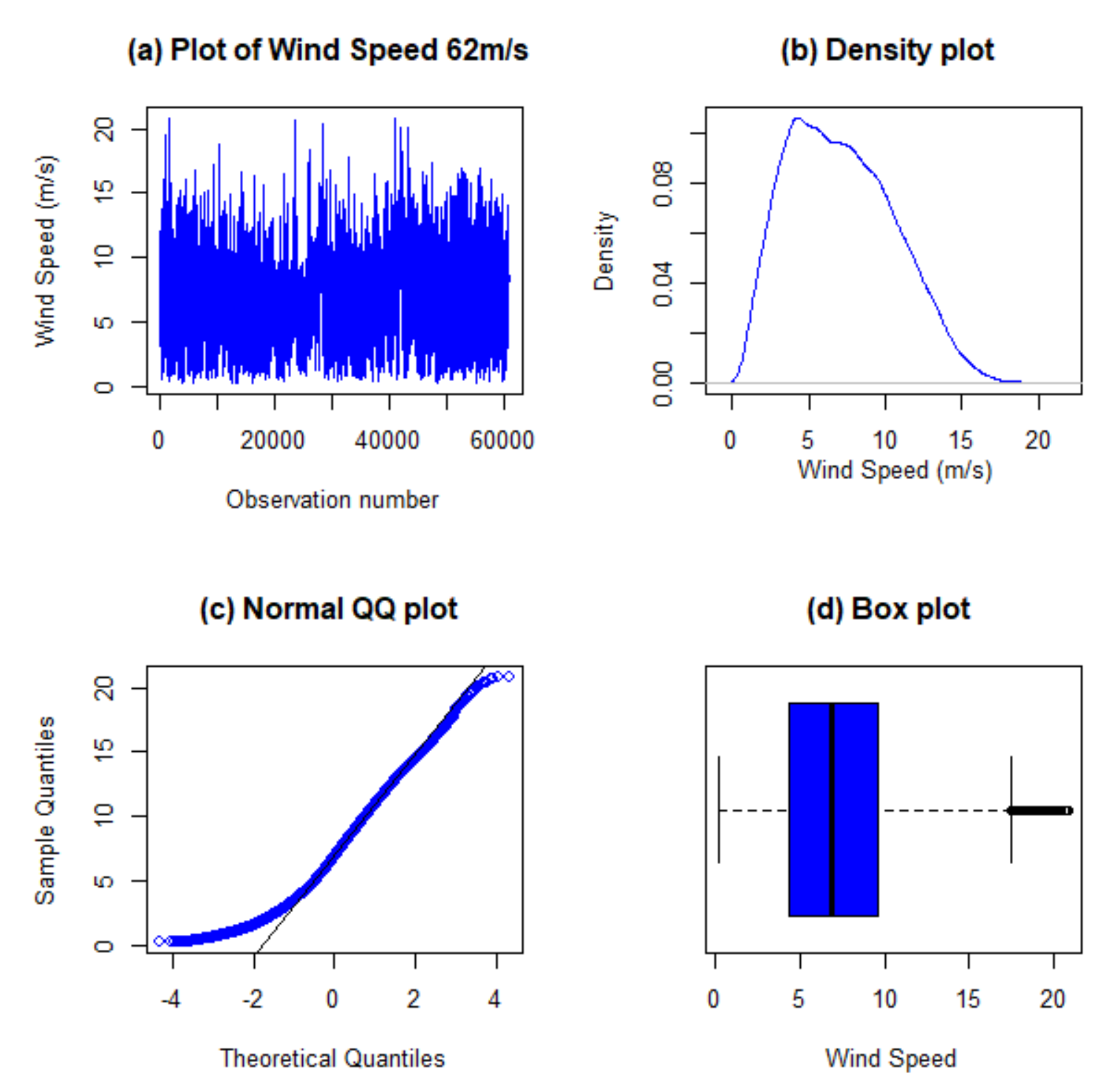
Table 2 shows that the distribution of the wind speed measured at 62 m WT hub is right skewed and platykurtic, as seen in the skewness and kurtosis values, hence not normally distributed. Another reason for the non-normality assertion is that the mean and median have different values. Time series plot, density, QQ (normal quantile to quantile) and box plots in Figure 2 all show that the response variable (wind speed at 62 m) distribution is not normally distributed.
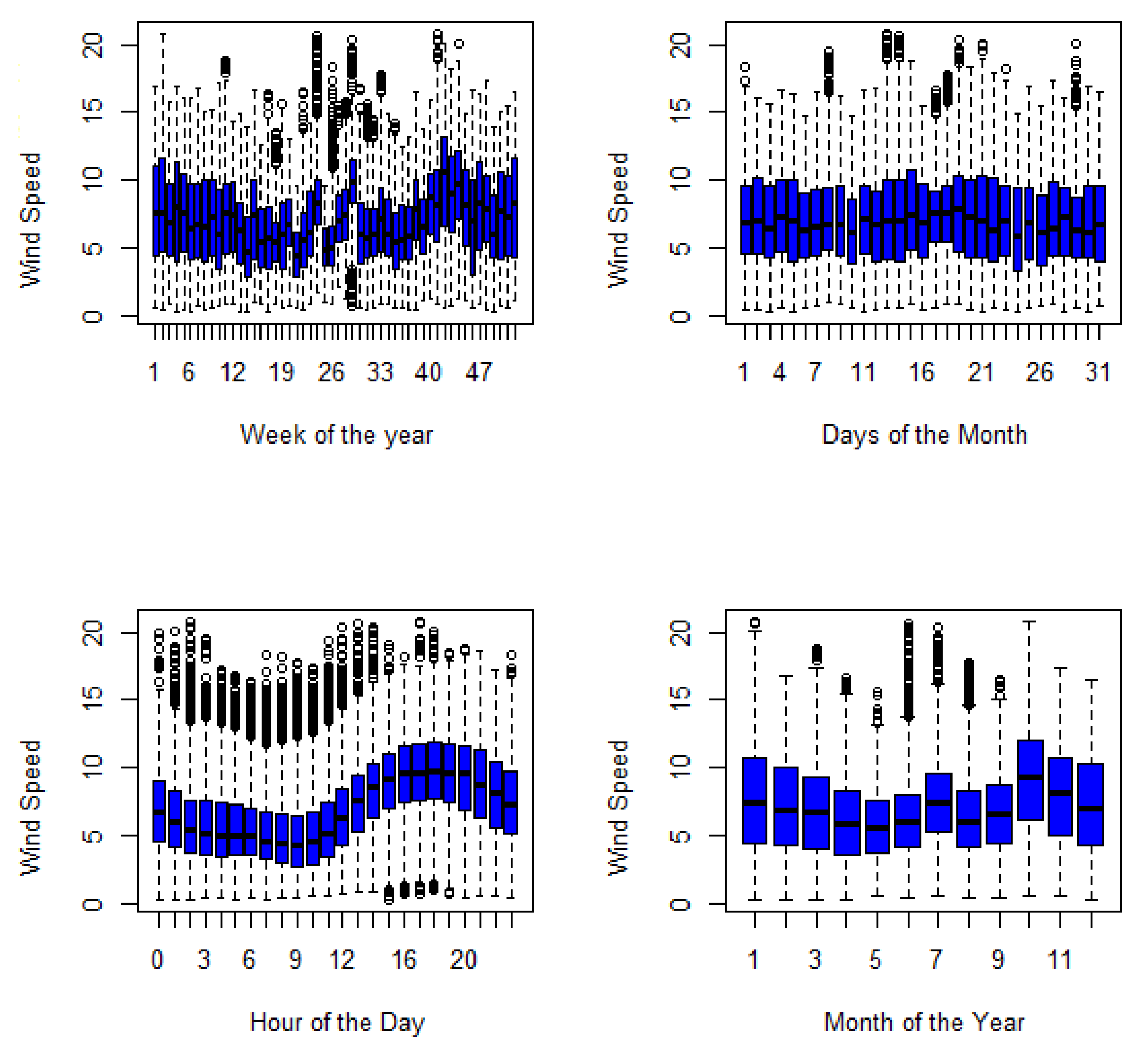
We also visualised the variations in the wind speed measured at 62 m altitude of the WT to envisage the possibility of forecasting it. The visualisation was carried out using box plots, shown in Figure 3. As shown in Figure 3, various patterns that are expected from the unpredictable nature of the wind speed are visible. There are no clear patterns visible when visualised in terms of the weeks in the year and the days of the month, other than the availability of the wind speed. However, the hours of the day and the months of the year show some clear patterns. Seasonal variation can be inferred from the months of the year box plots, and a trend can be seen from the hours of the day box plots. The 10th month corresponding to the peak of the spring season (in South Africa) has the largest wind speed, as seen in the month of the year box plots. The wind speed is seen to progress from the early hours of the day to the later hours of the day. The box plots show that wind speed is available throughout the days, however in varying and unpredictable quantity. This further shows how viable the wind speed is for generating renewable energy.
3.3. Results of Variable Selection
The needed predictor variables from the 48 variables in the dataset were selected using the least absolute shrinkage and selector operator (Lasso). Lasso in the Python 3 programming tool was implemented using the standard Lasso (Lasso) and the cross validation Lasso (Lassocv). Lassocv proved more robust than Lasso because it selected more variables for its variable selection. Lasso using the R programming tool on the other hand was implemented using the “glmnet” library for the benchmark models’ variable selection. A comparison of variable selection for the models is summarised in Table 3.
Table 3 gives the selected variables along with their coefficients from these two programming tools. For Lassocv from the Python 3 kernel, the selected 14 variables were added with the other lagged variables and used for the ANN model. In addition, the benchmark (BMLasso) model from the R kernel selected 10 variables; the lagged variables were added to the selected variables and used for both the GAM and SGB models, respectively. The lagging was done for 10-min lag, 1-h lag, one-day lag and two-day lag. In all variable selection processes, only 10-min lag was selected by the various Lasso variable selection processes.
SGB, being one of the benchmark models, ensures a form of variable selection in its working principle. Out of the 10 variables selected by Lasso, this model selected variables based on their relative importance for its computation. Table 4 shows the selected variables from SGB.
3.4. Point Forecasting Results
3.4.1. Benchmark Models’ Point Forecasts
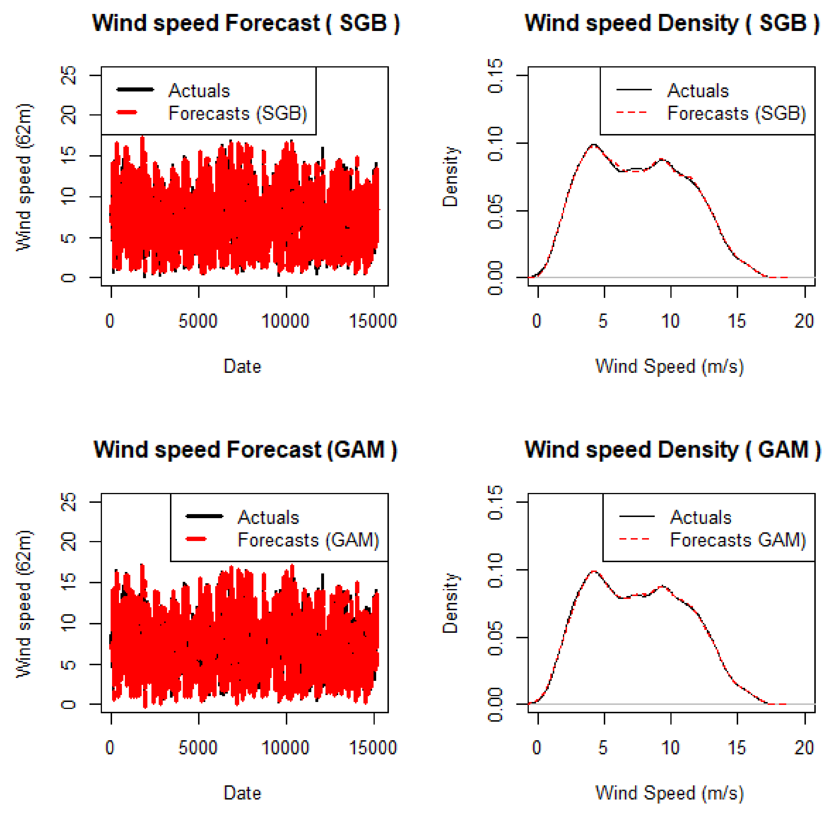
The benchmark models used the same set of variables selected by Lasso for their computation on R. The Libraries “caret” and “gbm” were used for the SGB while the “mgcv” library was used for fitting the GAM. A visualisation of the point forecasts produced from the test set given the training set using these models is shown in Figure 4. The dataset was split into training and test set in the ratio of 75%/25% for all three individual forecasting models.
In Figure 4, the highest wind speed (at 62 m hub height of the WT) values for both the actual and forecasts hovers around 20 m/s. We can also infer that the wind speed very close to 5 m/s is the densest plot of the wind speed with a density value very close to or a bit above 0.10. In the density plot, the lines showing the actual point forecast values and the lines showing the benchmark models’ point forecasts values are very close, indicating the performance of the models in forecasting. This reflects a considerable acceptable performance for the two benchmark models. Table 5 presents a summary of the accuracy metrics.
3.4.2. Artificial Neural Network and Additive Quantile Regression Averaging
This section presents the results of using the ANN and the main forecasts combination algorithm (AQRA) for point forecasting. ANN was implemented using the computational tool known as the Python 3 programming language. Following the steps from data curation to data explorations and visualisations along with data normalisation, this model is ready to carry out predictions from the variables selected by the LassoCV model. The ANN model was constructed from the SKLearn Library by importing MLPRegressor. The major determinants of an ANN are the number of layers in the network, the number of hidden layers and the number of nodes used for the hidden layer. ANN was constructed using three layers of input, hidden and output. The number of the hidden layers was made to be 1 by default, and the number of nodes in the hidden layer was given as 5. This makes the neural network thus constructed similar to the Bayesian Neural Network (BNN) in the work of Mbuvha [16]. In a BNN, the values of the and are very crucial, which are between 0 and 1 for a BNN. We thus performed hyper-parameter tuning to find the best values, best parameter and best accuracy making use of the GridSearchCV from the SKLearn model selector library.
AQRA, on the other hand, is a model formed from combining point forecasts from the other models. This model was fitted with forecasts from the BNN and the benchmark models (GAM and SGB) as its predictor variables, while the response variable is the point forecasts of the AQRA model. It was implemented using “qgam” library developed by Fasiolo et al. [42] on the R computational tool. The AQRA model was set at a seed of 1000 and functions such as tune-learn-fast as its object containing the actual forecasts and the point forecasts from the other three models fitted at a quantile value of . Plots of the point forecasts from ANN and AQRA models are shown in Figure 5. Other necessary visualisations from these two models and the rest are shown in Appendix A (Figure A1, Figure A3 and Figure A4).
In Figure 5, it is noticed that the highest wind speed forecast lie between 15 and 20 m/s and the highest dense plot for the wind speed is at a position very close to 5 m/s with a density of a little above 0.10. These two density plots also present these two models as viable models for wind speed forecasting because of the proximity of the actual and point forecasts values as represented by the two lines in the density plots. The density plot shows the densest point of the air in which an increasing wind speed gives a decline in its density until it returns to zero. The air density relates proportionally to the power realisable from the wind turbine [2,49].
The forecasts from these four models show the wind speed values lie in the range of 5–20-m/s. This corresponds to the linearly progressing and constant power region of the power curve of a wind turbine in [4]. This shows that both the actual values and the values from forecasts are within the range of values where electric power is being generated from the WT. A strong, increasing and constant electrical energy can thus be realised from the wind speed values, which depicts the richness of this renewable energy for generating electrical power.
3.5. Forecasts Accuracy Measures
3.5.1. Point Forecasts Accuracy Measures
This section presents the accuracy measures for our point forecasting models. This study made use of five forecasting models. The main model is the ANN model and compared with two benchmark models, SGB (a machine learning model) and GAM (a statistical learning model). The other two models are statistical models called additive quantile regression averaging and linear quantile regression averaging (LQRA). They are used to generate results from the point forecasts combination of the other three models. We present three accuracy metrics to evaluate these five point forecasting models. The various accuracy of point forecasts from these models are presented in Table 5.
In Table 5, model BNN is the first model whose forecasts is from the ANN, the second model is the SGB forecasts, the third model is the GAM forecasts, while the fourth and fifth models are the forecasts combination models, which are the AQRA forecasts and the forecasts corresponding to the LQRA model, respectively. Our discussion evaluates Table 5 with regards to individual and combined models, respectively.
BNN made use of 14 variables from its Lassocv variable selection model to fit the neural networks. It recorded the lowest RMSE value followed by GAM amongst the individual point forecasting methods. SGB, on the other hand, recorded the lowest MAE value followed by BNN while GAM recorded the highest MAPE value followed by BNN. Hence, accuracy measures using MAE and MAPE present SGB as the best individual point forecasting model followed by BNN while the GAM performed the least amongst these three models.
Considering the combined forecasting models, the fourth model, which is AQRA, performed better than its counterpart fifth model, which is LQRA, in all accuracy metrics axis. AQRA also outperformed all of the individual point forecasting models, as shown in Table 5. This is in tandem with most literature findings that combining point forecasts presents forecasts whose accuracy measures are lower than the individual forecasting models [19,20,21]. These findings hold sway for both methods of forecasts combination, as can be seen from their accuracy metrics’ values, which are lower than that of the three individual accuracy metrics’ values for the point forecasting models. When we combine forecasting models, the resultant combined forecasts perform better than the individual point forecasting models. Hence, the authors retain AQRA as the main forecast combination model for interval forecasting, while we drop LQRA going forward.
3.5.2. Prediction Interval Width
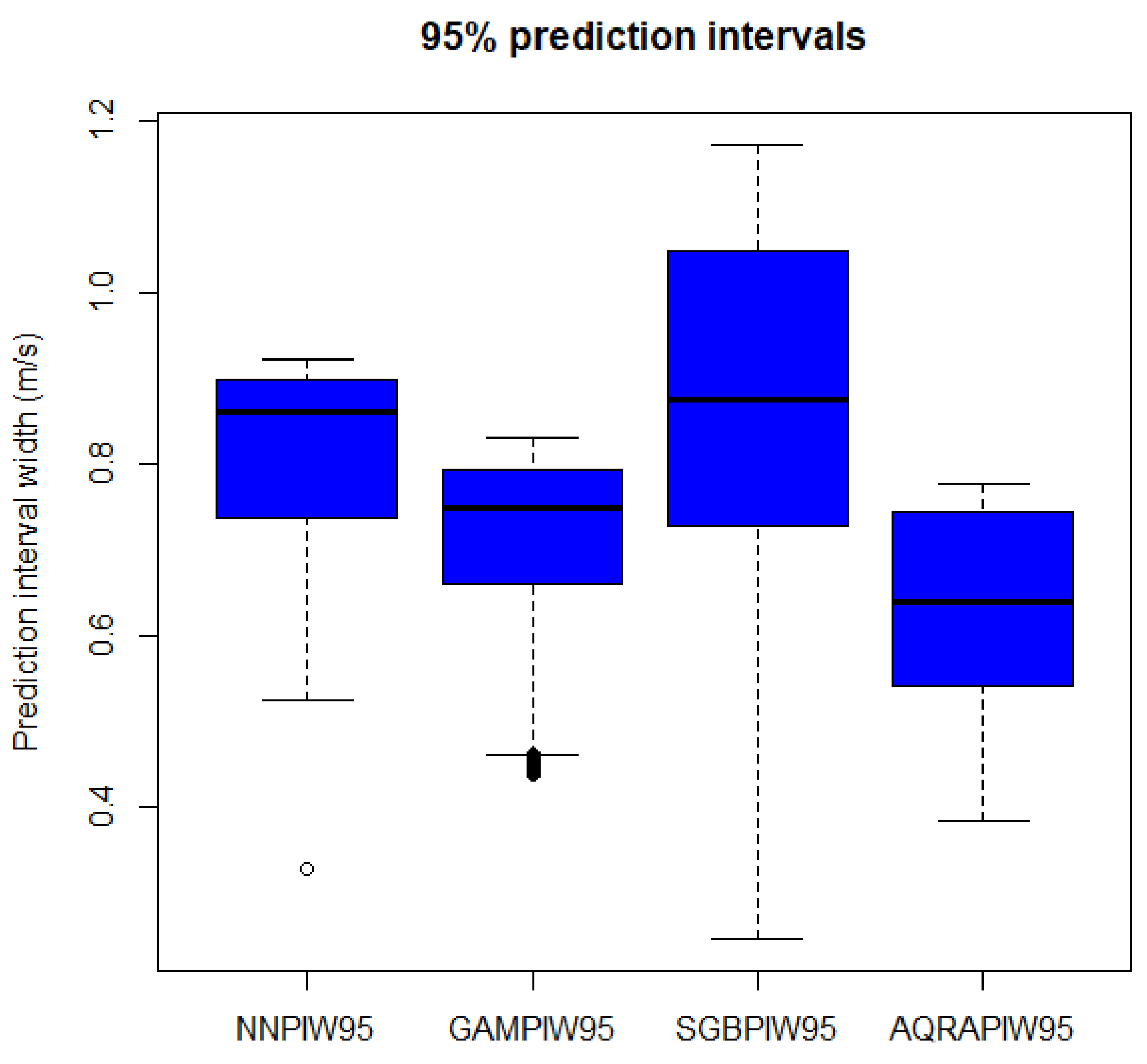
The analysis of the prediction interval width (PIW) at 95th quantile is presented in this section. Table 6 gives the summary statistics of the generated PIW, which gives the nature of the PI generated.
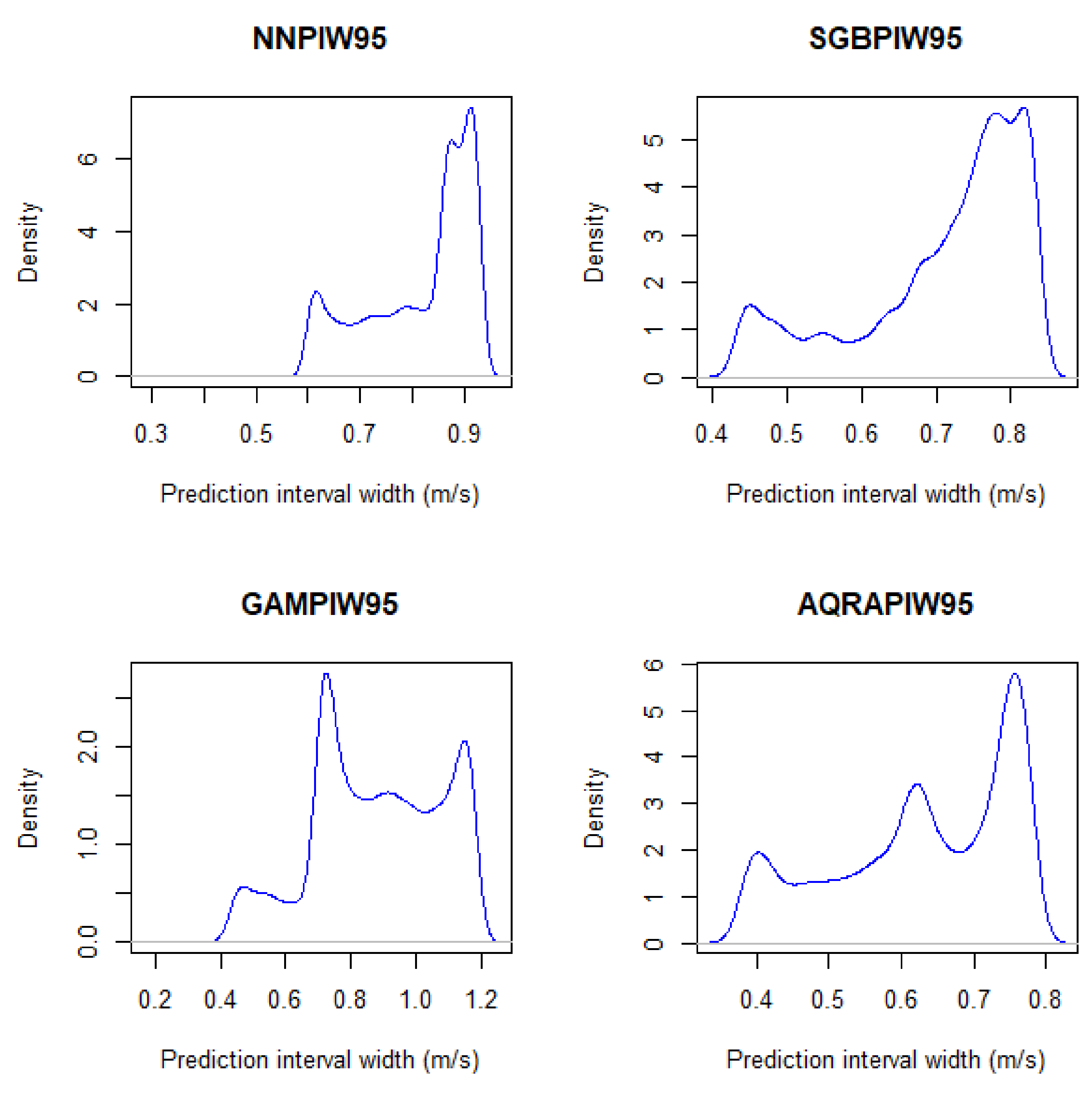
In Table 6, BNN has the least standard deviation followed by SGB, hence, PIW from these two models are narrower than those from AQRA and GAM, respectively. The skewness measures the distribution of a model and shows in the table that PIWs are not normally distributed, although close to a normal distribution (except SGB), because a normal distribution has a skewness value of 0. All of the models are also negatively skewed, showing that they are left-skewed. The kurtosis value for distribution is expected to be 3 and all kurtosis values for the models show them to be negative and less than 3, and they are therefore said to be platykurtic. The visualisation for PIW is presented in Figure 6. The figure presents PIW from AQRA as the most symmetrical and best model followed by SGB. BNN and GAM are skewed and much narrower than the other two. The PIW visualisation using the density plots in Figure 7, shows model BNN as the model with the narrowest intervals.
3.6. Prediction Intervals Evaluation
Forecasting using models is known to be filled with much uncertainties given good point forecasts performance evaluation. In this section, the methods for quantifying the uncertainties in point forecasting models as well as in the combined point forecasting model are described. To measure uncertainties, the needed feature to be used is the prediction interval. Along with making use of AQRA for forecast combination, it was also used to construct prediction intervals through the lower and upper bound estimates for the models and at different quantiles [21]. The quantiles considered are the 90th, 95th and 99th quantiles, respectively.
To quantify uncertainties, five prediction interval evaluation metrics were used in this study and the results are summarised in Table 7. The five metrics are the prediction interval nominal coverage (PINC), the prediction interval coverage percentage (PICP), the prediction interval normalised average width (PINAW), the prediction interval normalised average deviation (PINAD) and the prediction interval coverage average normalised width (PICAW). The theoretical formulations of these metrics are given in Section 2 (Equations (19) and (21)–(26)). These uncertainty metrics relating to quantifying the uncertainty in wind speed forecasting, using the individual point forecasting models and the AQRA forecasting combination model through the use of AQRA to construct prediction intervals whose values according to these metrics, are presented in Table 7.
In Table 7, five metrics are used to evaluate PIs from individual and the combined models. Four models in total are evaluated using these metrics. PICP is used to ascertain the reliability of the constructed PIs. Therefore, the more the actual values are covered by the PI, the higher are the PICP values [21]. Furthermore, PICP value is expected to be greater or equal to the PINC or confidence value else deemed as invalid [20]. Accurate and satisfactory PI performance is indicative of higher PICP values and lower PINAW values [20,21]. Both PICP and PICAW values indicate the quality of the constructed PI. Hence, a high PICP value with small PICAW value is required for a quality PI construction [21]. In addition, given a high PICP, the deviation value of the PIs from the actual value is expressed by PINAD. Hence, a higher PICP should give a lower PINAD value, showing less deviation from the actual value [31].
The discussion for Table 7 follows from the foregoing theoretical and literature findings. Using PICP at 90% PINC, all forecasts are valid and AQRA has the highest value and presents more coverage than the rest of the models. SGB is next and the last is BNN showing that the PI from BNN covers less actual values than the rest. Taking PICP and PINAW, AQRA presents both the highest PICP value and the lowest PINAW, thus the most reliable model at this confidence level. This is followed by BNN and the least is GAM. Although the PI from BNN covers fewer actual values, the covered values present a more closely fit weight than SGB and GAM. Taking PICP and PICAW, AQRA is the model with the best quality PI since it has the lowest PICAW value and the highest PICP value followed by BNN and the least is SGB. The degree of deviation from the actual value is shown by PINAD and BNN has the least degree of deviation followed by AQRA; GAM has the highest degree of deviation from the actual value. The ABLL and AAUL columns represent the number of actual values that are not within the range of PIW. They represent the number of actual values that are below the lower limit and the actual values that are above the upper limit, respectively.
For the 95% confidence value, SGB recorded the highest PICP value, GAM is next and then AQRA, while BNN has the lowest PICP value. At the 99% confidence values, SGB and BNN give higher PICP values than GAM and AQRA. The PICAW and PINAW values present AQRA as the best model followed by an interchange of SGB and BNN, respectively, while GAM remains constantly the least considering these two confidence values. Using PINAD, BNN has the best degree of deviation, and then AQRA followed by an interchange between SGB and GAM, respectively. The number of target values outside of the lower and upper limit range keeps reducing as the confidence level increases. AQRA is thus the best model at 90% confidence value; however, best models are evaluated based on what these metrics measures such as validity, reliability, quality and degree of deviation at a particular confidence value.
3.6.1. Evaluation of Combined Prediction Intervals
Just as point forecasts can be combined and estimate the evaluation of its accuracy, prediction intervals can also be combined and estimate the accuracy of the resultant combined PI. In this study, we made use of two prediction interval combination methods, the simple average and the median method, to produce a combined PI. Simple average gets the arithmetic mean of the PIs from individual models using the lower and upper bound estimate. A row-wise summation of the lower and upper limits is carried out and averaged by taking each model at the three quantiles considering the total number of models used. The mathematical formulation is given in Equation (27). The median method also follows the simple average method. We take the median values of all the models considered at a particular quantile. The mathematical expression is given in Equation (28). Table 8 presents the combined prediction interval evaluation using the same metrics as the individual PI model evaluation.
In Table 8, the simple average prediction interval combination method gives better PI than the median method at the 90% and 95% confidence values using PICP. However, it gives an invalid PI at the 99% confidence level recording a value smaller than the confidence level value, while the median method gave a satisfactory coverage value for its PICP. The median method provided reliable and better quality PI than the simple average method since it records lower values for its PINAW and PICAW at the 90% and 95% confidence levels. The 99% confidence value presents the median method as better than the average method using PINAW, while PICAW shows the opposite. The PINAD value for the 90% confidence level records a tie for the two combination methods, while the median method recorded the best value for its degree of deviation using PINAD at the 95% and 99% confidence levels. Lastly, an increment was seen in the number of PI, not within the lower and upper limit range for the two methods at the 90% and 95% confidence values. The 99% confidence value shows more number of actuals below the lower limit. These present the median method as the best PI combination method over the simple average method.
3.6.2. Residual Analyses
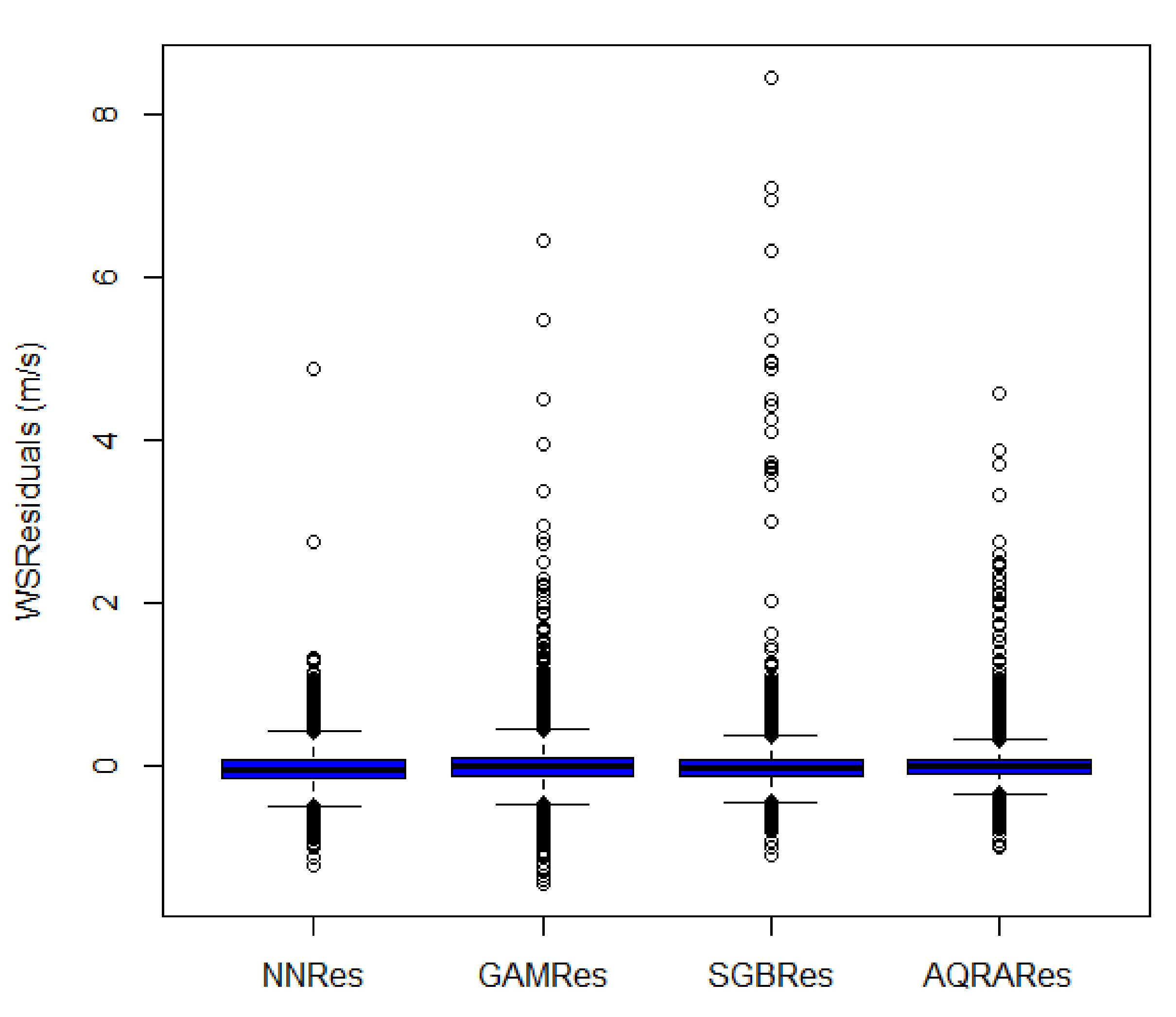
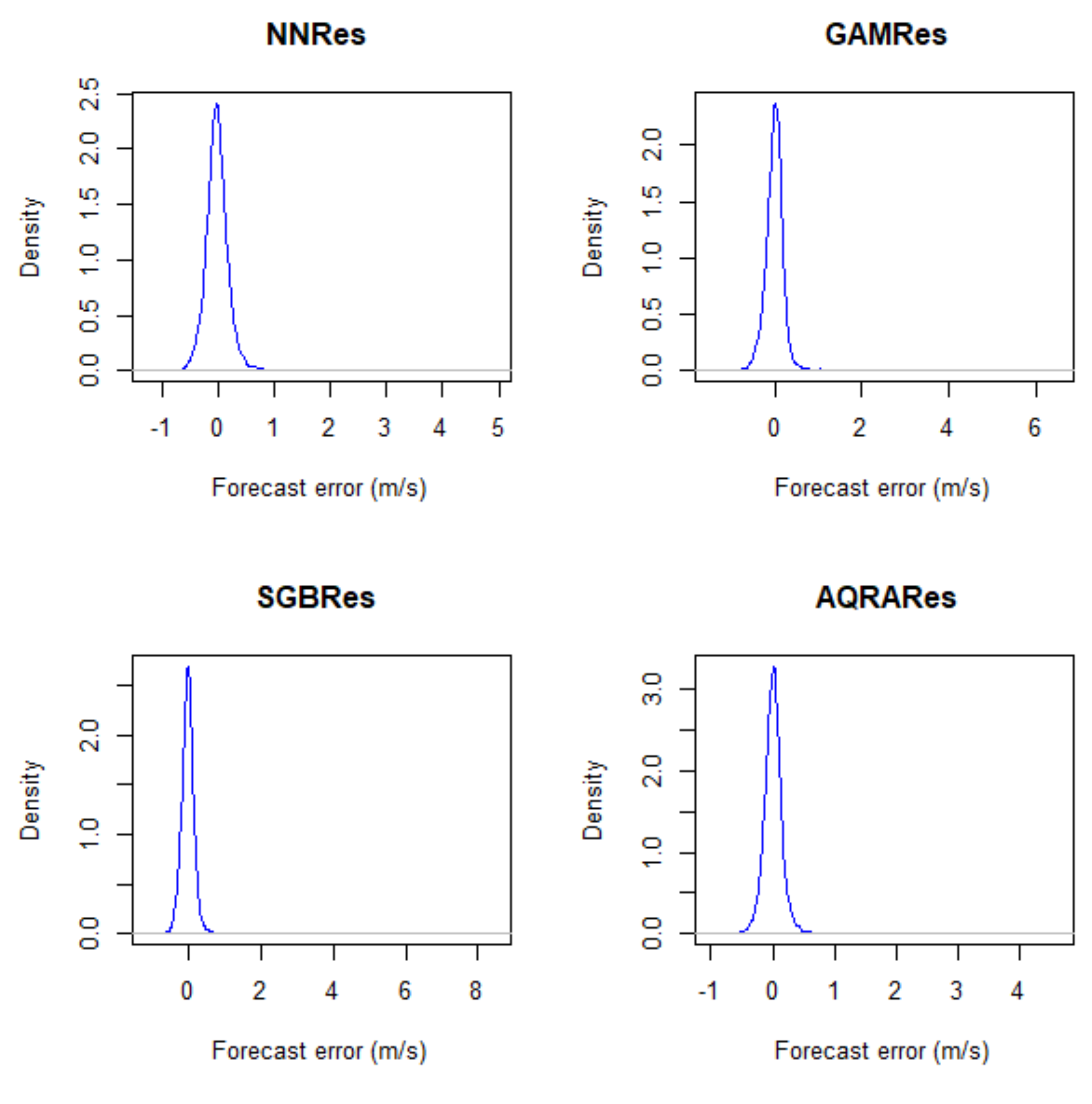
The summary statistics of errors or residuals for the models are shown in Table 9. The table shows model AQRA as having the least standard deviation, which means that its error distribution is the narrowest of all the models, as can also be seen in the box plot of Figure 8. This shows that the best model is AQRA in comparison to the others. The minimum values are all negative and the skewness values are far from being normally distributed. The kurtosis value shows erratic patterns; however, since they are all more than 3, they are termed leptokurtic data. The density plot in Figure 9 shows similar patterns and not much information can be inferred from these plots, except that they are all in between the −1 and +1 regions in the forecast error axis.
4. Discussion
This study was geared towards investigating methods useful for forecasting short-term unpredictable and intermittent wind speed for power generation. The method with smaller errors indicates the most accurate and desirable method. Two approaches were investigated: individual forecasting models and forecast combination models. Amongst the individual models, the Bayesian NN for the ANN was compared with two benchmark models involving SGB (ML method) and GAM (SL method). The evaluation of these three methods presented ANN as the best using RMSE while SGB is the best from MAE and MAPE forecast accuracy measures. On the other hand, two forecast combination methods, both of which are statistical methods, were investigated for the forecast combination and AQRA performed better than LQRA. It further outperformed the individual forecasts containing three methods (ANN and the two benchmark models) using all three forecast accuracy metrics involving RMSE, MAE and MAPE. Therefore, the authors present AQRA from forecasts combination as the best method for point forecasting of wind speed having lesser error values and the most accurate model.
Moving on to the prediction interval uncertainty measure, using only AQRA, the first uncertainty measure was the prediction interval width. Using this metric, our analysis at 95% confidence level shows that the model AQRA was the most symmetrical and the best model followed by SGB, even though ANN and GAM presented narrower prediction intervals than the others. None of these models gave a normal distribution and were all platykurtic. The research investigated further on interval forecasts, checking prediction intervals against the target values. Three confidence levels were considered: 90%, 95% and 99%. All the interval forecasts were checked for their validity, reliability, quality and degree of deviation from the actual values. All the models were valid models since PICP values were greater than the predetermined confidence levels. AQRA presented more reliable prediction intervals at 90%, having the highest coverage value. In addition, this constructed prediction interval at this level of confidence was deemed accurate and having satisfactory performance and quality since the lowest PINAW and PICAW values were recorded by AQRA followed by ANN. However, PINAD value shows ANN as the model with the least deviation. Actual values below and above the lower and upper limit kept decreasing, showing AQRA with the least values.
Forecasts from the SGB model have the highest coverage at the 95% confidence level followed by GAM. Using PINAW and PICAW for quality, accurate and satisfactory performance evaluation presented AQRA as the best model, while ANN and AQRA have the least degree of deviation. Constant reduction was noticed with the actual values below and above the lower and upper limits, respectively. The 99% confidence level shows SGB as the most reliable from its highest PICP value followed by GAM while the quality, accurate and satisfactory performance PI was seen to be AQRA from its PINAW and PICAW values. The least deviation was noticed in ANN followed by AQRA. The actual values below and above the lower and upper limit showed no consistency at this confidence level. The best model is AQRA followed by SGB. Analysis from the interval combination method is also reported. We used the simple average method and the median method. The simple average gave an invalid PICP at the 99% confidence level. The median method outperformed the simple average method in all prediction interval (accuracy measurement) metrics considered and, thus, the best interval combination method. The residual analysis also presents AQRA as the best, having the narrowest error non-normal distribution along with the other models.
5. Conclusions
This paper proposes a comparative analysis of statistical and machine learning methods along with their combination to two days ahead short-term wind speed point and interval forecasting. Various techniques that have been used for diverse forms of forecasting and forecast combinations along with uncertainty measures were explored. The use of GAM for other forms of forecasting but not for wind speed forecasting is the main gap filled by this work. Different mathematical underpinnings of these models and accuracy metrics along with uncertainty metrics serve as the methods and materials employed in this paper. Accuracy measures and uncertainty metrics were used to select the best models. In most of the discussions, it was found that the model AQRA, which is the additive quantile regression average method, is the best model for wind speed forecasting using both the point forecasts accuracy metrics (such as MAE, RMSE and MAPE) and the prediction intervals uncertainty measures involving PIW, PINC, PICP, PICAW, PINAW and PINAD. Hence, forecasts combination tends to improve short-term wind speed forecasting. Quantifying uncertainty in forecasts can assist the grid’s proper planning for scheduling of resultant power incorporation and dispatch. Future areas of study involve exploring other machine learning or deep learning algorithms for point forecasting, forecasts combination, prediction interval construction, and combination in wind speed/power forecasting.
Author Contributions
Conceptualisation, L.O.D. and C.S.; methodology, L.O.D., and C.S.; software, L.O.D., C.S. and R.M.; validation, L.O.D., C.S., C.C. and R.M.; formal analysis, L.O.D. and C.S.; investigation, L.O.D., C.S., C.C., and R.M.; resources, L.O.D., and C.C.; data curation, L.O.D.; writing—original draft preparation, L.O.D. and C.S.; writing—review and editing, C.S., C.C. and R.M.; visualisation, L.O.D. and C.S.; supervision, C.S., C.C. and R.M.; project administration, C.S., C.C.; and funding acquisition, L.O.D., and C.C. All authors have read and agreed to the published version of the manuscript.
Funding
This research was funded by the DST-CSIR National e-Science Postgraduate Teaching and Training Platform (NEPTTP) (www.escience.ac.za).
Acknowledgments
The support of the DST-CSIR National e-Science Postgraduate Teaching and Training Platform (NEPTTP) towards this research is hereby acknowledged. Opinions expressed and conclusions arrived at are those of the authors and are not necessarily to be attributed to the NEPTTP. In addition, we are grateful to the Wind Atlas South Africa (WASA) for providing the data (http://wasadata.csir.co.za/wasa1/WASAData).
Conflicts of Interest
The authors declare no conflict of interest. The funders had no role in the design of the study; in the collection, analyses, or interpretation of data; in the writing of the manuscript, or in the decision to publish the results.
Abbreviations
The following abbreviations are used in this manuscript:
| AI | Artificial Intelligence |
| ANN /NN | Artificial Neural Network / Neural Network |
| BNN | Bayesian Neural Network |
| ML | Machine Learning |
| SL | Statistical Learning |
| SGB | Stochastic Gradient Boosting |
| GAM | Generalized Additive Model |
| L/QR/A | Linear/ Quantile Regression / Averaging |
| Lasso | Least Absolute Shrinkage and Selector Operator |
| LassoCV | Least Absolute Shrinkage and Selector Operator with Cross validation |
| AQRA | Additive Quantile Regression Averaging |
| ARIMA | Auto-Regressive Integrated Moving Average |
| SARIMA/X | Seasonal Auto-Regressive Integrated Moving Average/for Exogenous Variable |
| PI | Prediction Interval |
| PIW | Prediction interval Width |
| PICP | Prediction Interval Coverage Probability |
| PINC | Prediction Interval Nominal Coverage |
| PINAW | Prediction Interval Normalised Average Width |
| PICAW | Prediction Interval Coverage Average -Normalised Average |
| PINAD | Prediction Interval Normalised Average Deviation |
| N/RMSE | Normalized / Root Mean Square Error |
| N/MAE | Normalized / Mean Average Error |
| MAPE | Mean Average Percentage Error |
| ABLL | Actual Below Lower Limit |
| AAUP | Actual Above Upper Limit |
| WASA | Wind Atlas South Africa |
| WT | Wind Turbine |
Appendix A. Visualizations for the BNN and AQRA
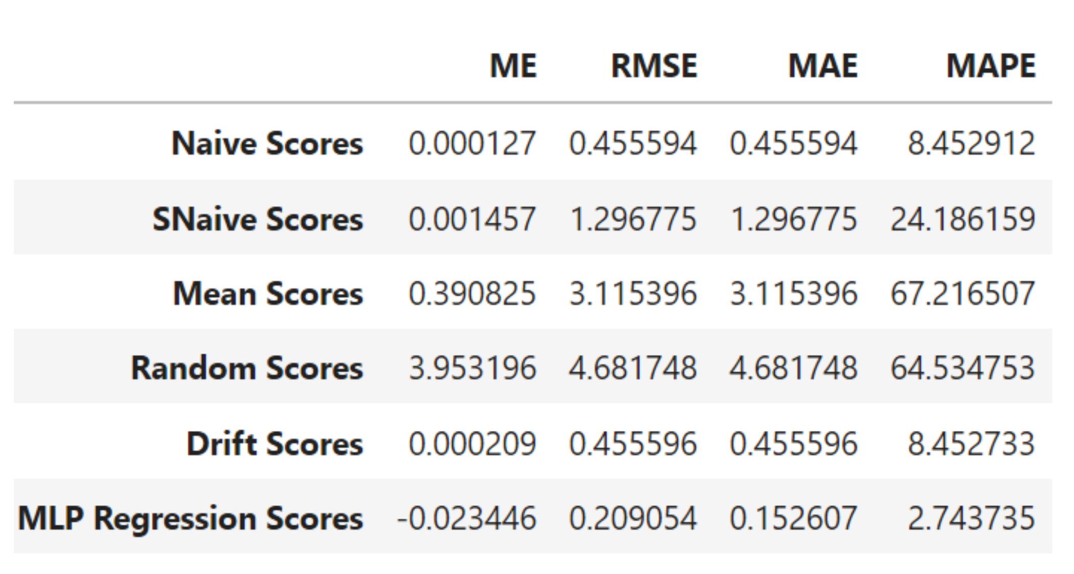
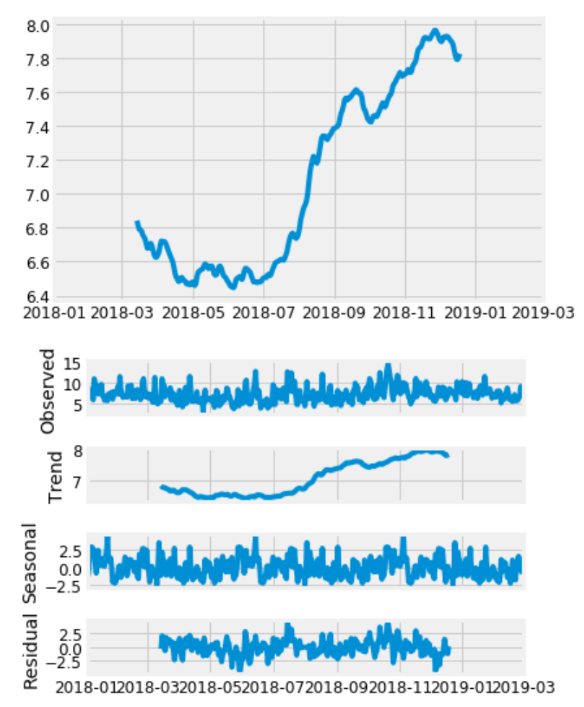
Figure A1 shows a comparison of the scores for different simple forecasting models and our BNN represented with MLPregressor using the forecast evaluation metrics. Figure A2 shows the extended plot of the period in the decomposition for the response variable (WS_62_mean) along some other necessary time series plots such as observed, trend, seasonal, and residuals. All these plots informed the choice of the dataset for location WM03 on WASA.
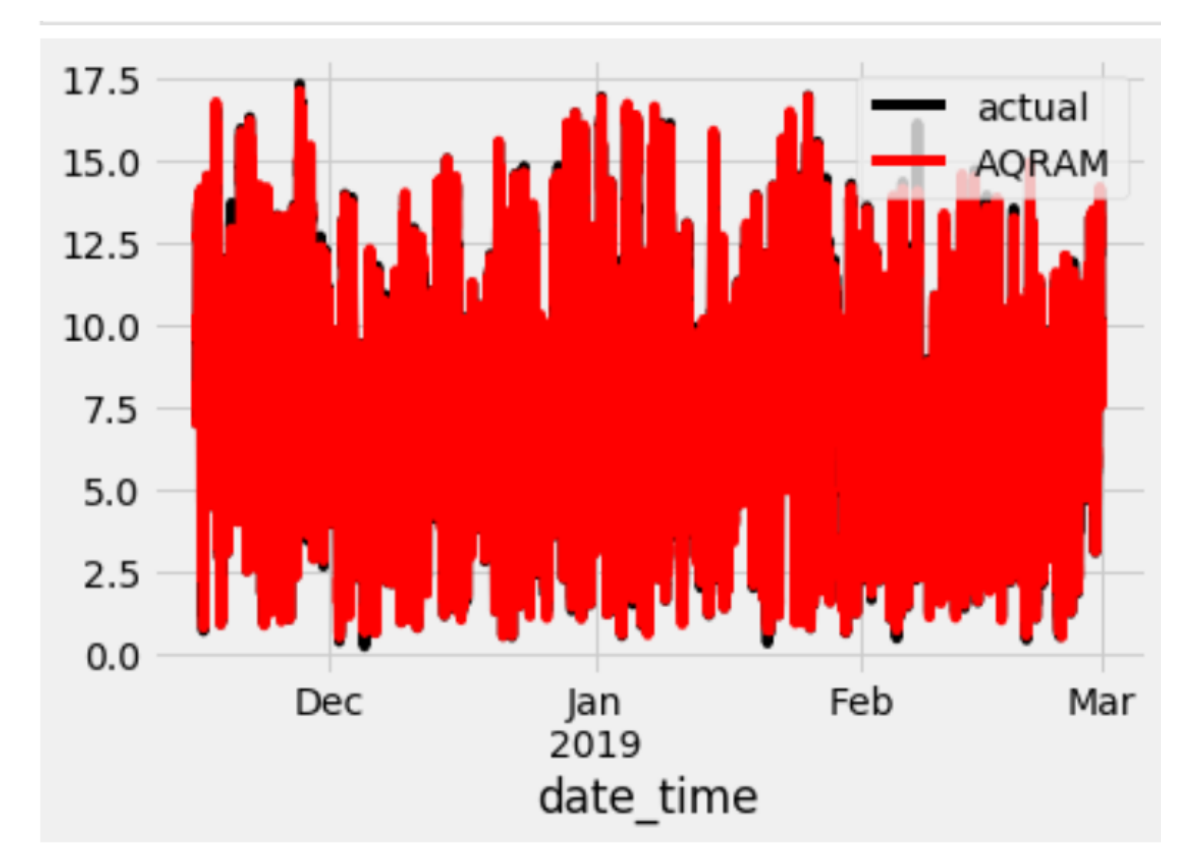
The plot of the actual forecast and the Additive quantile regression average model (AQRAM) is displayed in Figure A3 while the observation of the actual and the other four models used in the study is shown in Figure A4. The y-axis is the wind speed, the x-axis is the date_time of the test set. They all show a complete forecast with the colour representing the GAM forecasts more pronounced than that of the other models.
Figure A1.
Scores for the simple forecasts and BNN

Figure A2.
Decomposition of the Response Variable (WS_62_mean).

Figure A3.
Test set plot of wind speed (m/s) (y-axis) and the date_time (x-axis) for the AQRAM.

Figure A4.
Test set plot of wind speed (m/s) (y-axis) and the date_time (x-axis) for all the Models.
Figure A4.
Test set plot of wind speed (m/s) (y-axis) and the date_time (x-axis) for all the Models.

Appendix B. Variable Selection Metrics Using Lasso for BNN and SGB
Various Model variable selection evaluation metrics are presented in this appendix. The Lasso and the Lassocv from the Python kernel are compared in Table A1 while the SGB model variable selection was also evaluated using some known statistical evaluation metrics, as shown in Table A2.

Table A1.
Comparison between Lasso and Lassocv for the BNN.
| Metric | Lasso | Lassocv |
|---|---|---|
| Data Split ratio | 0.75/0.25 | 0.75/0.25 |
| Number of Variables selected | 10 out of 47 | 14 out of 47 |
| Training Score | 0.9859 | 0.9964 |
| Testing Score | 0.98565 | 0.9963 |
| Training data MSE | 0.1704 | 0.0431 |
| Testing data MSE | 0.1736 | 0.0447 |
Table A2.
SGB computational model evaluation.
| Interaction.depth | n.trees | RMSE | R-2quared | MAE |
|---|---|---|---|---|
| 1 | 50 | 0.5661520 | 0.9800269 | 0.3959074 |
| 1 | 100 | 0.3781487 | 0.9883580 | 0.2662815 |
| 1 | 150 | 0.3302557 | 0.9908337 | 0.2339422 |
| 2 | 50 | 0.3850630 | 0.9885786 | 0.2712526 |
| 2 | 100 | 0.2699944 | 0.9938029 | 0.1930438 |
| 2 | 150 | 0.2418027 | 0.9949749 | 0.1750470 |
| 3 | 50 | 0.3110675 | 0.9922893 | 0.2177381 |
| 3 | 100 | 0.2260250 | 0.9956210 | 0.1625230 |
| 3 | 150 | 0.2000053 | 0.9965582 | 0.1454654 |
References
- Lin, T.C. Application of Artificial Neural Network and Genetic Algorithm to Forecasting of Wind Power Output. Master’s Thesis, University of Jyväskylä, Jyväskylä, Finland, 2007. [Google Scholar]
- Chen, Q.; Folly, K.A. Comparison of Three Methods for Short-Term Wind Power Forecasting. In Proceedings of the IEEE 2018 International Joint Conference on Neural Networks (IJCNN), Rio de Janeiro, Brazil, 8–13 July 2018; pp. 1–8. [Google Scholar]
- Pinson, P. Wind energy: Forecasting challenges for its operational management. Stat. Sci. 2013, 28, 564–585. [Google Scholar] [CrossRef] [Green Version]
- Barbosa de Alencar, D.; de Mattos Affonso, C.; Lim ao de Oliveira, R.; Moya Rodríguez, J.; Leite, J.; Reston Filho, J. Different models for forecasting wind power generation: Case study. Energies 2017, 10, 1976. [Google Scholar] [CrossRef] [Green Version]
- Abhinav, R.; Pindoriya, N.M.; Wu, J.; Long, C. Short-term wind power forecasting using wavelet-based neural network. Energy Procedia 2017, 142, 455–460. [Google Scholar] [CrossRef]
- Ferreira, M.; Santos, A.; Lucio, P. Short-term forecast of wind speed through mathematical models. Energy Rep. 2019, 5, 1172–1184. [Google Scholar] [CrossRef]
- Morina, M.; Grimaccia, F.; Leva, S.; Mussetta, M. Hybrid weather-based ANN for forecasting the production of a real wind power plant. In Proceedings of the IEEE 2016 International Joint Conference on Neural Networks (IJCNN), Vancouver, BC, Canada, 24–29 July 2016; pp. 4999–5005. [Google Scholar]
- Giebel, G.; Kariniotakis, G. Wind power forecasting—A review of the state of the art. In Renewable Energy Forecasting; Elsevier: Amsterdam, The Netherlands, 2017; pp. 59–109. [Google Scholar]
- Verma, S.M.; Reddy, V.; Verma, K.; Kumar, R. Markov Models Based Short Term Forecasting of Wind Speed for Estimating Day-Ahead Wind Power. In Proceedings of the IEEE 2018 International Conference on Power, Energy, Control and Transmission Systems (ICPECTS), Chennai, India, 22–23 February 2018; pp. 31–35. [Google Scholar]
- Sebitosi, A.B.; Pillay, P. Grappling with a half-hearted policy: The case of renewable energy and the environment in South Africa. Energy Policy 2008, 36, 2513–2516. [Google Scholar] [CrossRef]
- Yan, J.; Liu, Y.; Han, S.; Gu, C.; Li, F. A robust probabilistic wind power forecasting method considering wind scenarios. In Proceedings of the 3rd Renewable Power Generation Conference (RPG 2014), Naples, Italy, 24–25 September 2014. [Google Scholar]
- Sigauke, C.; Nemukula, M.; Maposa, D. Probabilistic Hourly Load Forecasting Using Additive Quantile Regression Models. Energies 2018, 11, 2208. [Google Scholar] [CrossRef] [Green Version]
- Chen, Y.; Ding, Y.; Ding, J.; Chen, Z.; Sun, R.; Zhou, H. A statistical approach of wind power forecasting for grid scale. AASRI Procedia 2012, 2, 121–126. [Google Scholar]
- Zhu, B.; Chen, M.Y.; Wade, N.; Ran, L. A prediction model for wind farm power generation based on fuzzy modeling. Procedia Environ. Sci. 2012, 12, 122–129. [Google Scholar] [CrossRef] [Green Version]
- Baghirli, O. Comparison of Lavenberg-Marquardt, Scaled Conjugate Gradient and Bayesian Regularization Backpropagation Algorithms for Multistep Ahead Wind Speed Forecasting Using Multilayer Perceptron Feedforward Neural Network. Master’s Thesis, Uppsala University, Uppsala, Sweden, 2015. [Google Scholar]
- Mbuvha, R. Bayesian Neural Networks for Short Term Wind Power Forecasting. Master’s Thesis, School of Computer Science and Communication, KTH Royal Institute of Technology, Stockholm, Sweden, 2017. [Google Scholar]
- Liu, B.; Nowotarski, J.; Hong, T.; Weron, R. Probabilistic load forecasting via quantile regression averaging on sister forecasts. IEEE Trans. Smart Grid 2015, 8, 730–737. [Google Scholar] [CrossRef]
- Wang, L.; Wang, Z.; Qu, H.; Liu, S. Optimal forecast combination based on neural networks for time series forecasting. Appl. Soft Comput. 2018, 66, 1–17. [Google Scholar] [CrossRef]
- Nowotarski, J.; Weron, R. Computing electricity spot price prediction intervals using quantile regression and forecast averaging. Comput. Stat. 2015, 30, 791–803. [Google Scholar] [CrossRef] [Green Version]
- Sun, X.; Wang, Z.; Hu, J. Prediction interval construction for byproduct gas flow forecasting using optimized twin extreme learning machine. Math. Probl. Eng. 2017, 2017, 5120704. [Google Scholar] [CrossRef] [Green Version]
- Shen, Y.; Wang, X.; Chen, J. Wind power forecasting using multi-objective evolutionary algorithms for wavelet neural network-optimized prediction intervals. Appl. Sci. 2018, 8, 185. [Google Scholar] [CrossRef] [Green Version]
- Abuella, M.; Chowdhury, B. Hourly probabilistic forecasting of solar power. In Proceedings of the IEEE 2017 North American Power Symposium (NAPS), Morgantown, WV, USA, 17–19 September 2017; pp. 1–5. [Google Scholar]
- Zhang, Y.; Wang, J.; Wang, X. Review on probabilistic forecasting of wind power generation. Renew. Sustain. Energy Rev. 2014, 32, 255–270. [Google Scholar] [CrossRef]
- Liu, H. Generalized Additive Model; Department of Mathematics and Statistics University of Minnesota Duluth: Duluth, MN, USA, 2008. [Google Scholar]
- Goude, Y.; Nedellec, R.; Kong, N. Local short and middle term electricity load forecasting with semi-parametric additive models. IEEE Trans. Smart Grid 2014, 5, 440–446. [Google Scholar] [CrossRef]
- Pierrot, A.; Goude, Y. Short-term electricity load forecasting with generalized additive models. In Proceedings of the ISAP Power, Hersonissos, Greece, 25–28 September 2011. [Google Scholar]
- Cho, H.; Goude, Y.; Brossat, X.; Yao, Q. Modeling and forecasting daily electricity load curves: A hybrid approach. J. Am. Stat. Assoc. 2013, 108, 7–21. [Google Scholar] [CrossRef] [Green Version]
- Shadish, W.R.; Zuur, A.F.; Sullivan, K.J. Using generalized additive (mixed) models to analyze single case designs. J. Sch. Psychol. 2014, 52, 149–178. [Google Scholar] [CrossRef]
- Zhang, G.; Patuwo, B.E.; Hu, M.Y. Forecasting with artificial neural networks: The state of the art. Int. J. Forecast. 1998, 14, 35–62. [Google Scholar] [CrossRef]
- Friedman, J.H. Stochastic gradient boosting. Comput. Stat. Data Anal. 2002, 38, 367–378. [Google Scholar] [CrossRef]
- Mpfumali, P.; Sigauke, C.; Bere, A.; Mulaudzi, S. Day Ahead Hourly Global Horizontal Irradiance Forecasting—Application to South African Data. Energies 2019, 12, 3569. [Google Scholar] [CrossRef] [Green Version]
- Friedman, J.H. Greedy function approximation: A gradient boosting machine. Ann. Stat. 2001, 29, 1189–1232. [Google Scholar] [CrossRef]
- Hastie, T.; Tibshirani, R.; Friedman, J.; Franklin, J. The elements of statistical learning: Data mining, inference and prediction. Math. Intell. 2005, 27, 83–85. [Google Scholar]
- Hastie, T.; Tibshirani, R. Generalized Additive Models; CRC Press: Boca Raton, FL, USA, 1990; Volume 43. [Google Scholar]
- Pya, N.; Wood, S.N. A note on basis dimension selection in generalized additive modelling. arXiv 2016, arXiv:1602.06696. [Google Scholar]
- Bates, J.M.; Granger, C.W. The combination of forecasts. J. Oper. Res. Soc. 1969, 20, 451–468. [Google Scholar] [CrossRef]
- Hoeting, J.A.; Madigan, D.; Raftery, A.E.; Volinsky, C.T. Bayesian model averaging: A tutorial. Stat. Sci. 1999, 14, 382–401. [Google Scholar]
- Sigauke, C. Forecasting medium-term electricity demand in a South African electric power supply system. J Energy S. Afr. 2017, 28, 54–67. [Google Scholar] [CrossRef]
- Taieb, S.B.; Huser, R.; Hyndman, R.J.; Genton, M.G. Forecasting uncertainty in electricity smart meter data by boosting additive quantile regression. IEEE Trans. Smart Grid 2016, 7, 2448–2455. [Google Scholar] [CrossRef]
- Maciejowska, K.; Nowotarski, J.; Weron, R. Probabilistic forecasting of electricity spot prices using Factor Quantile Regression Averaging. Int. J. Forecast. 2016, 32, 957–965. [Google Scholar] [CrossRef]
- Gaillard, P.; Goude, Y.; Nedellec, R. Additive models and robust aggregation for GEFCom2014 probabilistic electric load and electricity price forecasting. Int. J. Forecast. 2016, 32, 1038–1050. [Google Scholar] [CrossRef]
- Fasiolo, M.; Goude, Y.; Nedellec, R.; Wood, S.N. Fast calibrated additive quantile regression. arXiv 2017, arXiv:1707.03307. [Google Scholar] [CrossRef] [Green Version]
- Wang, Y.; Zhang, N.; Tan, Y.; Hong, T.; Kirschen, D.S.; Kang, C. Combining probabilistic load forecasts. IEEE Trans. Smart Grid 2018, 10, 3664–3674. [Google Scholar] [CrossRef] [Green Version]
- Lim, M.; Hastie, T. Learning interactions via hierarchical group-Lasso regularization. J. Comput. Graph. Stat. 2015, 24, 627–654. [Google Scholar] [CrossRef]
- Hastie, T.; Tibshirani, R.; Wainwright, M. Statistical Learning with Sparsity: The Lasso and Generalizations; Chapman and Hall/CRC: London, UK, 2015. [Google Scholar]
- Plan, Y.; Vershynin, R. The generalized Lasso with non-linear observations. IEEE Trans. Inf. Theory 2016, 62, 1528–1537. [Google Scholar] [CrossRef]
- Brown, B.G.; Katz, R.W.; Murphy, A.H. Time series models to simulate and forecast wind speed and wind power. J. Clim. Appl. Meteorol. 1984, 23, 1184–1195. [Google Scholar] [CrossRef]
- Landberg, L. Short-term prediction of the power production from wind farms. J. Wind. Eng. Ind. Aerodyn. 1999, 80, 207–220. [Google Scholar] [CrossRef]
- Olaofe, Z.O. Wind Energy Generation and Forecasts: A Case Study of Darling and Vredenburg Sites. Ph.D. Thesis, University of Cape Town, Cape Town, South Africa, 2013. [Google Scholar]
Figure 1.
Vredendal map location (Source: https://www.weather-forecast.com/locationmaps/Vredendal.10.gif).
Figure 1.
Vredendal map location (Source: https://www.weather-forecast.com/locationmaps/Vredendal.10.gif).

Figure 2.
Diagnostic plots for the response variable, WS_62_mean.

Figure 3.
Distribution of Wind Speed (m/s) across the week, month, day and year in the dataset.

Figure 4.
Benchmark density and point forecasts plots.

Figure 5.
ANN and AQRA density and point forecasts plots.

Figure 6.
PIW of BNN-AQRA.

Figure 7.
Density plots for PIW of BNN through AQRA.

Figure 8.
Box plots of residuals.

Figure 9.
Density Plots of Residuals.

Table 1.
Summary of models, description and motivations.
| Model | Description | Motivation |
|---|---|---|
| ANN, SGB and GAM | Machine and Statistical learning, Deterministic methods | Point forecasting |
| LQRA and AQRA | Statistical and Probabilistic Methods | Forecasts combination and Prediction interval construction |
| The LASSO | Mathematical | Variable/feature selection |
| MAE, RMSE, and MAPE | Mathematical | Point forecast evaluation metrics |
| PIW, PICP, PINAW, PINAD and PICAW | Mathematical formulations and Interval forecasting metrics | To quantify uncertainties in the forecasts |
| Simple Average and Median PI | Mathematical | Prediction Interval combination (Improves forecast) |
Table 2.
Summary statistics of the response variable WS_62_mean (m/s).
| Min | 1st Qu | Median | Mean | 3rd Qu | Max | Std. | Skewness | Kurtosis |
|---|---|---|---|---|---|---|---|---|
| 0.2134 | 4.3674 | 6.8670 | 7.1725 | 9.6473 | 20.8555 | 3.475177 | 0.3963677 | −0.4654862 |
Table 3.
Variables and their coefficients from the Lasso.
| Variable | ANN Lasso | ANN Lassocv | BMLasso |
|---|---|---|---|
| WS_62_min | 0.088897 | 0.314418 | 3.643221 × |
| WS_62_max | 0.410781 | 0.337446 | 2.614169 × |
| WS_60_mean | 0.253464 | 0.120781 | 1.454732 × |
| WD_60_mean | 0.000287 | 0.000134 | 9.436018 × |
| WD_60_min | – | 0.000068 | – |
| WD_60_max | −0.000591 | 0.000007 | – |
| WD_60_stdv | −0.015175 | −0.005907 | −4.402683 × |
| WD_20_mean | 0.000834 | 0.000048 | – |
| WD_20_stdv | −0.001630 | — | – |
| RH_min | −0.000793 | 0.000169 | – |
| lag1 | 0.119809 | 0.094290 | 8.940951 × |
| WS_40_mean | – | 0.148194 | 1.581057 × |
| WD_20_min | – | −0.000036 | – |
| WD_20_max | – | 0.000082 | – |
| WS_60_stdv | – | – | 2.898686 × |
| Tair_min | – | 0.000590 | −7.744566 × |
| Tair_mean | – | – | −2.311307 × |
| Total No of Variables | 10 | 14 | 10 |
Table 4.
Variable selection by the SGB model.
| Selected Variable | Relative Importance |
|---|---|
| WS_40_mean | 4.379310 × |
| WS_60_mean | 4.117128 × |
| WS_62_max | 1.411519e × |
| WD_60_mean | 4.687078 × |
| WD_60_stdv | 3.892787 × |
| WS_60_stdv | 6.227314e × |
| Tair_min | 1.768753 × |
| Tair_mean | 0.000000 × |
Table 5.
Accuracy measures for the point forecasting models.
| Model | No of Used Variables | RMSE | MAE | MAPE |
|---|---|---|---|---|
| BNN | 14 | 0.2091 | 0.1526 | 2.7437 |
| SGB | 8 | 0.2553 | 0.1397 | 2.3754 |
| GAM | 10 | 0.2468 | 0.1579 | 3.0356 |
| AQRA | 3 | 0.1888 | 0.1167 | 2.0330 |
| LQRA | 3 | 0.1928 | 0.1204 | 2.0986 |
Table 6.
Summary statistics for PIW at 95th quantile.
| Model | Min | Max | Mean | Median | St.Dev | Skewness | Kurtosis |
|---|---|---|---|---|---|---|---|
| BNN | 0.3281 | 0.9217 | 0.8148 | 0.8613 | 0.1016 | −0.7914 | −0.7346 |
| SGB | 0.4378 | 0.8313 | 0.7099 | 0.7487 | 0.1124 | −1.0610 | −0.0271 |
| GAM | 0.2461 | 1.1725 | 0.8762 | 0.8744 | 0.1952 | −0.2188 | −0.7905 |
| AQRA | 0.3843 | 0.7759 | 0.6277 | 0.6399 | 0.1213 | −0.5330 | −0.9302 |
Table 7.
Prediction Interval Evaluation.
| PINC% | Model | %PICP | %PINAW | %PICAW | %PINAD | ABLL | AAUL |
|---|---|---|---|---|---|---|---|
| 90 | BNN | 90.4956 | 3.7853 | 8.3489 | 0.0130 | 717 | 727 |
| SGB | 90.6997 | 3.8336 | 8.4560 | 0.1101 | 701 | 712 | |
| GAM | 90.6334 | 3.8259 | 8.4432 | 0.1109 | 702 | 721 | |
| AQRA | 90.7194 | 2.8583 | 6.3140 | 0.0650 | 707 | 703 | |
| 95 | BNN | 95.2807 | 4.7673 | 10.5152 | 0.0388 | 358 | 359 |
| SGB | 95.4058 | 4.1536 | 9.1076 | 0.0659 | 348 | 341 | |
| GAM | 95.3992 | 5.1263 | 11.3586 | 0.0665 | 345 | 354 | |
| AQRA | 95.3926 | 3.6725 | 8.1101 | 0.0534 | 342 | 358 | |
| 99 | BNN | 99.0654 | 7.3491 | 16.1999 | 0.0083 | 72 | 70 |
| SGB | 99.0983 | 7.8238 | 17.9690 | 0.0298 | 66 | 71 | |
| GAM | 99.0259 | 8.8693 | 19.6512 | 0.0198 | 78 | 70 | |
| AQRA | 99.0588 | 7.1009 | 15.8021 | 0.0133 | 70 | 73 |
Table 8.
Combined prediction interval evaluation.
| PINC% | Model | %PICP | %PINAW | %PICAW | %PINAD | ABLL | AAUL |
|---|---|---|---|---|---|---|---|
| 90 | SAverage | 93.1743 | 3.5780 | 7.9661 | 0.0250 | 513 | 524 |
| Median | 92.3978 | 3.5510 | 7.8617 | 0.0250 | 579 | 576 | |
| 95 | SAverage | 97.1500 | 4.4299 | 9.9499 | 0.0370 | 198 | 235 |
| Median | 96.8012 | 4.2181 | 9.3775 | 0.0330 | 235 | 251 | |
| 99 | SAverage | 98.4137 | 7.7858 | 11.2930 | 0.0110 | 198 | 43 |
| Median | 99.3148 | 7.2292 | 16.7254 | 0.0044 | 52 | 48 |
Table 9.
Summary statistics for the residuals.
| Model | Min | Max | Mean | Median | St.Dev | Skewness | Kurtosis |
|---|---|---|---|---|---|---|---|
| BNN | −1.2156 | 4.8961 | 0.0235 | −0.0304 | 0.2077 | 1.4241 | 29.9048 |
| SGB | −1.1015 | 8.4607 | −0.0128 | −0.0180 | 0.2550 | 11.4720 | 273.8021 |
| GAM | −1.4350 | 6.4689 | 0.0028 | 0.0045 | 0.2468 | 4.0097 | 72.3618 |
| AQRA | −0.9845 | 4.5838 | 0.0061 | 0.0004 | 0.1887 | 4.9086 | 78.1724 |
© 2020 by the authors. Licensee MDPI, Basel, Switzerland. This article is an open access article distributed under the terms and conditions of the Creative Commons Attribution (CC BY) license (http://creativecommons.org/licenses/by/4.0/).
Share and Cite
MDPI and ACS Style
Daniel, L.O.; Sigauke, C.; Chibaya, C.; Mbuvha, R. Short-Term Wind Speed Forecasting Using Statistical and Machine Learning Methods. Algorithms 2020, 13, 132. https://0-doi-org.brum.beds.ac.uk/10.3390/a13060132
AMA Style
Daniel LO, Sigauke C, Chibaya C, Mbuvha R. Short-Term Wind Speed Forecasting Using Statistical and Machine Learning Methods. Algorithms. 2020; 13(6):132. https://0-doi-org.brum.beds.ac.uk/10.3390/a13060132
Chicago/Turabian StyleDaniel, Lucky O., Caston Sigauke, Colin Chibaya, and Rendani Mbuvha. 2020. "Short-Term Wind Speed Forecasting Using Statistical and Machine Learning Methods" Algorithms 13, no. 6: 132. https://0-doi-org.brum.beds.ac.uk/10.3390/a13060132
Note that from the first issue of 2016, this journal uses article numbers instead of page numbers. See further details here.