A Linear-Time Algorithm for the Isometric Reconciliation of Unrooted Trees


Department of Computer Science, Faculty of Mathematics, Physics, and Informatics, Comenius University, Mlynská dolina, 842 48 Bratislava, Slovakia
*
Authors to whom correspondence should be addressed.
Algorithms 2020, 13(9), 225; https://0-doi-org.brum.beds.ac.uk/10.3390/a13090225
Submission received: 15 July 2020
/
Revised: 28 August 2020
/
Accepted: 4 September 2020
/
Published: 8 September 2020
(This article belongs to the Special Issue Algorithms in Bioinformatics)
Abstract
:In the reconciliation problem, we are given two phylogenetic trees. A species tree represents the evolutionary history of a group of species, and a gene tree represents the history of a family of related genes within these species. A reconciliation maps nodes of the gene tree to the corresponding points of the species tree, and thus helps to interpret the gene family history. In this paper, we study the case when both trees are unrooted and their edge lengths are known exactly. The goal is to root them and to find a reconciliation that agrees with the edge lengths. We show a linear-time algorithm for finding the set of all possible root locations, which is a significant improvement compared to the previous algorithm.
1. Introduction
Reconciliation of gene trees and species trees is a computational problem arising in evolutionary biology that has been studied since 1979 [1]. Here, we concentrate on a variant proposed by Ma et al. [2,3], called isometric reconciliation. We provide a linear-time algorithm for reconciling two unrooted trees, which is a significant improvement over the previous algorithm [4].
A species tree represents an evolutionary history of a group of species. Present-day species are typically placed in the leaves, and internal nodes correspond to speciation events. Speciation is a process in which individuals of a single species separate into two groups that further evolve independently.
A gene tree represents an evolutionary history of a group of related genes from several species. In the simplest scenario, each individual has a single copy of a particular gene, and these genes are propagated along the species tree, yielding the gene tree identical to the species tree. However, during evolution, a gene can be lost (deleted), and it can also become duplicated, whereupon a particular species and its descendants have multiple copies of the gene. After a series of such duplication and deletion events, the gene tree and the species tree will differ. In a gene tree, the leaves represent copies of the gene in the present-day species and the internal nodes represent speciations and duplications. Lost gene copies are not represented in gene trees.
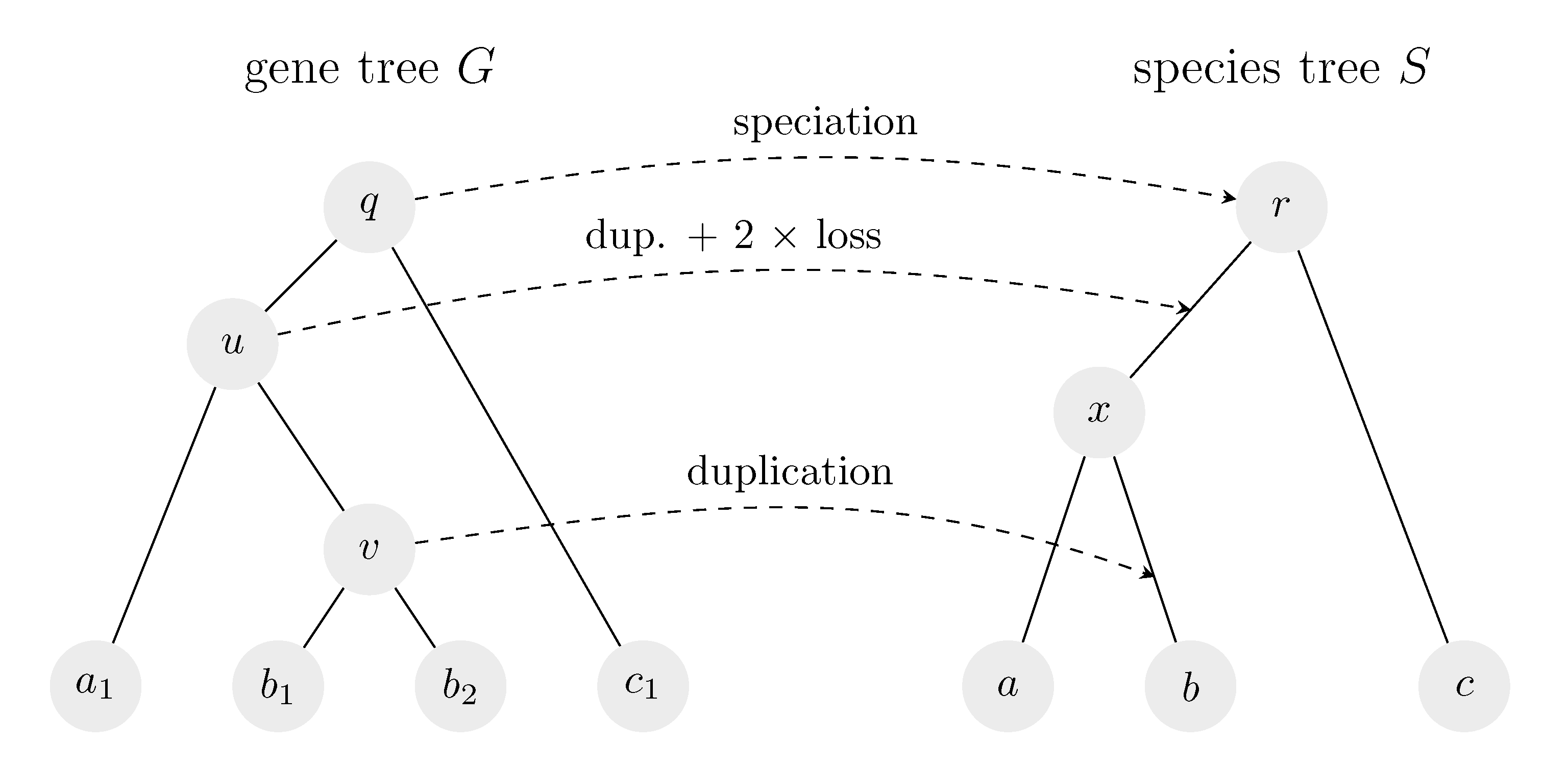
The goal of reconciliation is to map nodes of a gene tree to the corresponding points in a species tree that represent the same points in the evolutionary history. This mapping helps to distinguish whether a node of a gene tree corresponds to a speciation or a duplication and to estimate the number of deletions (see an example in Figure 1).
Note that gene trees and species trees representing evolutionary histories are rooted, with the root representing the last common ancestor of all the leaves. However, trees are in practice constructed from DNA or protein sequences, and many commonly used methods are unable to determine the root location, so instead provide only an unrooted version of the tree [5].
In the isometric reconciliation, both trees have known edge lengths and the reconciliation has to obey these lengths (see an example in Figure 2). The problem was introduced by Ma et al. [2,3], who provided a polynomial-time algorithm for reconciling an unrooted gene tree with a rooted species tree. Brejová et al. [4] have provided a corrected and improved version of this algorithm, which runs in time, where N is the total number of nodes in the two trees combined. The authors also provided algorithms for several variants of the problem, including an -time algorithm to compute all reconciliations of two unrooted trees. In this paper, we improve this running time to for gene trees with node degrees bounded by (typically, unrooted phylogenetic trees have internal nodes of degree three). To achieve this time, we only output pairs of valid root locations in the two trees instead of full reconciliations. Given any pair of such root locations, the full reconciliation can be computed in time by a simple algorithm given by Brejová et al. [4]. If the earlier algorithm [4] is modified to output only root locations, it still runs in time; thus the algorithm presented here is a significant improvement.
We also characterize the set of possible root locations, proving that it always forms a connected subgraph of the species tree and that the distances between different root locations in the species tree and their counterparts in the gene tree are preserved.
Finally, note that the problem of gene tree and species tree reconciliation was also studied in other settings [6]. The most traditional is the parsimony setting that uses unweighted trees and seeks a reconciliation minimizing the number of inferred duplications and deletions. This problem can be solved in linear time for two rooted trees [7,8]. For unrooted gene trees, it is possible to find all optimal root locations in linear time [9]. Rooting an unrooted species tree using a set of unrooted gene trees was also considered [10]. Edge lengths were used in the context of probabilistic models of gene duplication and deletion [11,12,13] and in models allowing horizontal transfer of genes between species [14,15].
In the rest of this section, we introduce necessary notation and formally define the isometric reconciliation problem. In Section 2, we describe our algorithm and supporting proofs, including the characterization of the solution set. We provide further discussion of our results and several open problems in Section 3.
1.1. Notation
A gene tree will be in the rest of the text denoted G, species tree S. Nodes of G are usually denoted as u and v, nodes of S as x and y, the root of G as q, the root of S as r and leaves in both trees as a and b.
A point in a tree is one of its nodes or a point inside an edge where this edge can be subdivided by a new node. By , we denote the distance between points u and v in tree T. For a tree T with nodes u and v and real value , such that , let denote the point located at distance from node u on the path connecting points u and v. By , we denote the lowest common ancestor of u and v in a rooted tree T.
Let be an edge in an unrooted tree T. By we will denote a rooted subtree of T obtained by removing edge from T, taking the resulting connected component containing u and rooting it in u. A tree with m edges thus has rooted subtrees. In rooted trees, we will consider subtrees in the conventional sense, consisting of a node and all its descendants.
For a tree T, let be the set of its leaves and the set of its nodes. For a tree T and a set of leaves A, let denote the subtree of T induced by A and all paths connecting pairs of leaves from A. In particular, we will often consider the subtree for some rooted subtree T of S; this is the part of G that naturally corresponds to subtree T of S.
1.2. Definition of Reconciliation
Consider a rooted or unrooted tree G (the input gene tree), rooted or unrooted tree S (the input species tree) and input mapping , which gives for each gene its species of origin. Both trees have edges weighted by non-negative weights. An isometric reconciliation of the triple is a triple , where and are weighted rooted trees and is a mapping from to such that the following holds:
- The output gene tree is either G, if G is rooted, or a rooted version of G obtained by subdividing some edge and rooting the tree in this newly created node.
- The output species tree is obtained from S by rooting it if S is unrooted and optionally subdividing some edges by additional nodes and also optionally adding a new path leading from above to the original root of S.
- Mapping agrees with input mapping on all leaves.
- Mapping preserves the ancestor/descendant relationships and the distances between ancestors and descendants. For each u and v such that u is a parent of v in , we have that is an ancestor of and .
- Nodes are not added to and unnecessarily. For each node x which was added to except for the root, there is some node u from such that . The edges incident to x have strictly positive weights.
Note that when subdividing a weighted edge , we divide the original edge length between the new edges so that the distance of u and v remains the same. The new nodes added to the output species tree represent duplication events; the path above the root of S corresponds to ancient duplications happening before the first speciation represented in the species tree. Figure 3 shows an example of an isometric reconciliation where the root of maps above the original root of . A more detailed discussion of the isometric reconciliation model can be found in the article by Brejová et al. [4].
For algorithmic simplicity, we allow rooting trees only in points located on edges, not in the original nodes. To root a tree in an existing node u, we choose one of the edges incident to u and subdivide it by a new node in the distance 0 from u. This is the only exception where we are allowed to create new edges of zero length.
In this paper, we do not compute the full reconciliation which includes mapping and new nodes added to the input trees. Instead, we output all pairs of valid roots in the two trees, that is, pairs of points in G and S such that when the trees are rooted in these points, they can be reconciled. If desired, the full reconciliation can be easily computed for any particular pair of valid roots in time.
As we will see in Section 2.7, valid roots in S form a set of intervals of points on individual edges; for edge in S we can express such an interval as the set of points for . For some edges, the set of valid roots can be empty, and for some it may contain only a single point. For each non-empty interval, we also have the corresponding interval of valid roots on some edge in G; this interval thus has the form for .
2. Algorithm
In this section, we describe our linear-time algorithm. A proof-of-concept implementation of this algorithm is available at https://github.com/fmfi-compbio/unrooted-reconciliation.
The previous work shows that for rooted species tree S and unrooted gene tree G, there is at most one root location in G so that the trees can be reconciled [2,4]. The key idea of our algorithm is to take individual rooted subtrees of an unrooted tree S and to compute for each the unique location of the root in the corresponding part of G (Section 2.4).
In the second phase of the algorithm (Section 2.5), we consider each edge of S as a possible root location and combine information from the two rooted subtrees at its endpoints to obtain an interval of positions along this edge where the root can be placed.
To keep the running time linear, our computation in the first two phases of the algorithm does not check all requirements of an isometric reconciliation; the final check in the third phase either validates or rejects all preliminary solutions (Section 2.6).
Finally, in the fourth phase, we compute for each root location in S its exact corresponding root location in G (Section 2.7).
2.1. Assumptions and Preprocessing
In the core of our algorithm, we make the following assumptions.
- The input trees G and S have the same set of leaves, and the input mapping is implicitly represented by leaf equality.
- All internal nodes of tree S have degree three; S may have zero-length edges.
- The degrees of all internal nodes of tree G are at least three and are bounded from above by some constant c; all edges of G have strictly positive lengths.
Of these assumptions, the first one may seem unrealistic, because reconciliation is typically performed on gene families where individual species have multiple copies, and thus the input mapping is a many-to-one mapping. However, we will show in Section 2.8 that this condition can be satisfied for any input trees by simple preprocessing.
The remaining conditions are satisfied for typical fully resolved phylogenetic trees with strictly positive edge lengths, but we also show how to handle a more general class of trees in preprocessing. The only serious obstacles are high-degree nodes either in the original G or resulting from contracting zero-length edges during preprocessing. Our algorithm works for high-degree nodes in G, but the running time becomes .
In the rest of the paper, we assume that any trees G and S satisfy the requirements outlined in this section. The algorithm works for unrooted input trees, but some claims will consider rooted species trees which occur in the algorithm as subproblems.
2.2. Tree Primitives
In our algorithm, we use the following algorithmic building blocks, whose efficient implementation is explained in Section 2.8. We work with points in the trees represented as for some nodes u and v in tree T and distance such that . The following statements assume that -time preprocessing is done on each input tree .
- Given two points u and v in tree T, we can compute their distance in time.
- Given three points u, v and w in a tree with strictly positive edge lengths, we can determine if v is located on the path connecting u and w in time; we denote this predicate .
- Given two points , and in tree T where , , , are nodes of T, we can represent point in the form where , and this representation can be computed in time.
- Given tree T with m edges, we can list all its rooted subtrees so that if node w is a child of u in a subtree ; then subtree occurs in the list before subtree . We call this ordering bottom-up order of the rooted subtrees, and it can be computed in time. If we process rooted subtrees in the bottom-up order, all subtrees of each rooted subtree are processed before itself.
2.3. Potential Rooting of a Gene Tree
In the first phase of our algorithm, we process all rooted subtrees of the species tree S and compute potential rootings of the corresponding parts of G, as defined in the next definition.
Definition 1.
Let S be a rooted species tree with root r and G an unrooted gene tree with the same set of leaves. A potential rooting of G with respect to S is a pair where q is a point in G and h is a real value such that for any leaf we have
The intuition behind this definition is that in the reconciliation of S with G, point q is the new root of G, and it maps to distance h above node r. In an isometric reconciliation, we always have , but here we allow negative values of h to keep the algorithm simple; negative values of h are ruled out in a later phase of the algorithm. In the rest of this section, we prove a series of claims characterizing potential rootings. Although Definition 1 and the following claims are formulated for rooted tree S, we will eventually apply them to rooted subtrees T of an unrooted tree S, and to keep the set of leaves the same, we will restrict G to .
Claim 1.
Let S be a rooted species tree with root r and G an unrooted gene tree. Then there is at most one potential rooting of G with respect to S. More precisely, ifandare potential rootings, thenand.
Proof.
Let , be two potential rootings. If , then both and must be equal to , where r is the root of S, and a is an arbitrary leaf from .
Therefore, let us assume that . Consider the forest obtained by removing the path connecting and from G. For , let us denote by an arbitrary leaf of G contained in the component of this forest containing . Due to the choice of leaf , the path from to in G goes through , and thus we obtain the following equations:
Symmetrically, for we have
which is a contradiction, implying that indeed . □
Claim 2.
Let S be a rooted species tree with root r and G an unrooted gene tree. Letbe a subtree of S with root. Letbe a potential rooting of G with respect to S. Thenhas a potential rootingwith respect to, whereis the point ofclosest to q (distance measured by). In particular, if q is inside, then. Valueis defined by the following equation:
Proof.
Let be the point of closest to q, and let be the value defined by Equation (1). Then for any leaf a of the path from a to q must lead through , and thus we have . Similarly, . By combining these two equations, the equation implied by the potential rooting and Equation (1), we obtain
Thus we have proved that is the potential rooting, as required. □
The following two claims help us to compute potential rootings.
Claim 3.
Let both S and G contain only a single node x. The potential rooting of G with respect to S is.
Claim 4.
Let S be a rooted species tree with root r, which is an internal node with two childrenand, and let G be an unrooted gene tree. Letandbe subtrees of S rooted atand. Let us assume thatandhave potential rootings,(both rootings exist). Then the pairis a potential rooting of G if and only if the following three conditions are satisfied.
- 1.
- .
- 2.
- , whereand.
- 3.
- Letbe the path in G betweenand. For eacheitheroris completely outsideexcept for its endpoint.
Proof.
Let and . Tree G consists of and and possibly the path connecting these two trees in G.
First, let us prove that if is a potential rooting, it satisfies the three conditions. Let us start with Condition 3 for some . If , the condition is automatically satisfied. Otherwise, we can use Claim 2 to observe that must be the point from closest to q, implying that the path from q to is outside except for . This discussion also implies that q is on the path from to , as needed in Condition 2.
Next, we use Equation (1) from Claim 2, which gives us the value of h expressed as
for each of the subtrees . We obtain the desired value of from Condition 2 directly from Equation (2) for , noting that . Finally, using Equation (2) for and noting that , we obtain Condition 1.
To prove that the three conditions imply potential rooting, we first prove that Conditions 1 and 2 imply for each . This equation clearly holds for from Condition 2 as . Therefore, let us consider . From definition of q in Condition 2, we see that . Then we use definitions of and h from Conditions 1 and 2, the fact that and simple manipulations to get
Now consider any leaf . We need to prove that . Let i be the index such that a belongs to . Thanks to Condition 3, we have that . Since is a potential rooting of , we have that . Finally, since , we have . These three observations yield the desired equality
□
2.4. Computation of Potential Rootings
In the first phase of the algorithm, we will compute potential rootings of all rooted subtrees of S. Claim 3 gives the potential rooting of a subtree with one leaf, and Claim 4 allows us to compute the potential rooting of a bigger subtree from rootings of its two subtrees.
Let T be a rooted subtree of S. The point q in a potential rooting of will be represented in the algorithm as for some leaves a and b and distance . We will also keep a set of representative leaves for each subtree with a potential rooting . The size of this set will be the same as the degree of q in . For each edge incident to q in , the set will contain a leaf a such that is true; that is, the path from q to a uses edge . Note that if q is not a node of G, but rather a point inside some edge e, we will assume that G was modified by subdividing e in this point, and thus the degree of q is two, and it has two incident edges.
The algorithm processes each rooted subtree T of S in the bottom-up order. As a special case, if consists only of leaf a, the rooting will be represented as , where , and the representative set is .
Consider now rooted subtree T with two rooted subtrees , as in Claim 4; we will also use other notation from the claim. The rooting for subtree T is computed from already known rootings of and as follows.
- Compute h using Condition 1 of Claim 4. This requires computing , where and are represented as and for some leaves , , . This distance computation is one of our tree primitives (see Section 2.2 and Section 2.8).
- Compute from Condition 2; check that . Then represent point in the form where . This computation is also one of our primitives.
- To check Condition 3, we use the sets of representative leaves and for and , respectively. We also build the set A for q (see Figure 4).If , Condition 3 is satisfied, and . To build the set A, we start with the union of and . This clearly covers all outgoing edges from q belonging to , but some of them may be covered twice, if they are shared between and . Thus, if for some and we have that is false, either or is excluded from A.Now let us assume that for some ; let j be the other index from . We need to check that the edge leaving from towards q and does not belong to . This is achieved by checking that for each leaf the predicate is true (see Figure 5). If neither nor equal q, this check is repeated for both values of i.To build the set A for q, we consider two cases: if q is one of the endpoints of the path between and , say , then we start with set and add to it one leaf from as a representative of the edge leaving from towards .Finally, if q is inside the path connecting and , its degree in will be two and the set A will consist of one arbitrarily chosen leaf from each and .A straightforward implementation of this step takes if and if . If the degree of each node of G is , the running time of this step is also .
If the degrees of all nodes of G are , the overall running time for computing potential rootings of all subtrees is .
2.5. Potential Roots of an Unrooted Species Tree
Once we have potential rootings computed for all rooted subtrees of an unrooted tree S, we can consider potential roots of S, defined as follows.
Definition 2.
Let G and S be unrooted. A point r in S is called a potential root of S if there exists some potential rooting of G with respect to S rooted at r.
For each edge of S, consider rooting tree S at the point for . This yields a rooted tree on which we can apply Claim 4, using precomputed potential rootings and for the two subtrees and of S rooted at and . Using this claim, we can compute for which values of we obtain a potential rooting of G with respect to .
In particular, Condition 1 of Claim 4 specifies the value of h which does not depend on the unknown distance . Condition 2 specifies the position q of the root in G, but for this position to be valid, value of must be from the specified interval. This translates to interval for . Possible values of also must be within edge , and thus we take an intersection of two intervals, yielding the following interval of possible values:
Note that this interval might be empty, signifying that no potential rooting exists, or it might contain only a single value of .
Finally, to satisfy Condition 3 of Claim 4 for , we consider two cases. If the path connecting and lies outside of except for the endpoints, we can place point q anywhere on this path without violating this condition. However, if some portion of this path is inside for some , we have to place q to , restricting possible values of to a single value (0 or , depending on i), and thus is also restricted to a single value or potentially to an empty set. Condition 3 has to be satisfied for both values of .
To algorithmically check whether is outside of , we again use the set of representative leaves for . For each leaf , we evaluate the predicate , where j is the index from different from i. If the predicate is true for all representative leaves, the path is outside.
The result of this phase of the algorithm is for every edge of S an interval of potential roots of S which yield potential rootings of G. The location of the root q is given in the form where is the distance of the root of S from node and f is a function of the form , where as discussed above.
2.6. Checking Distances
In the third phase of the algorithm, we are given a set of potential roots, and we need to verify whether they correspond to actual reconciliations. We do so based on comparing distances between pairs of selected leaves in trees S and G, as explained in the following two claims.
Note that the definition of isometric reconciliation requires that distances between a node of G and its descendants and ancestors are preserved by the mapping. However, for other pairs of nodes, the distance in G can be greater than the distance of the corresponding points in S. For example, in Figure 2 leaves and of G are at distance 8, but the corresponding leaves a and b from S have a distance of only 4. Next we show that the distances in G cannot be smaller than distances in S.
Claim 5.
Letbe an isometric reconciliation of a triple, where trees S and G can be either rooted or unrooted. Then for each two nodes u and v from G, we have.
Proof.
Note that the definition of isometric reconciliation implies that if u is an ancestor of v in G; then is an ancestor of and . Additionally, note that for any nodes u and v of G we have , and similarly, the distances remain preserved between S and .
Let and . Note that must be an ancestor of x, because it is an ancestor of both and .
□
Given a rooted tree T, let be the mapping which maps each node x of T to the smallest leaf in the subtree of T rooted at x under some fixed complete order on the set .
Claim 6.
Let S be a rooted tree and G an unrooted tree. Trees S and G can be reconciled if and only if the following two conditions hold:
- There is a potential rootingof G (letbe G rooted in q)
- For each two nodesandwhich are inchildren of the same node we have
Proof.
If the reconciliation exists, we can obtain the potential rooting by taking the root of as q and setting where r is the root of tree S. Inequality (8) is implied by Claim 5.
Let us now assume the existence of a potential rooting satisfying the two conditions. We will root tree G in q and construct the mapping as follows. Node q is mapped to the point located in distance h above the root of S; let us call this point r and denote tree S extended with r as . Each node v of the rooted is then mapped to . First of all, we need to prove that this mapping exists, in particular that . This is true because the definition of a potential rooting implies that , and since the path from q to passes through v, we have the desired inequality. Note that the leaves of are correctly mapped by to their counterparts in .
Next we prove that if v is an ancestor of w in and is an ancestor of in , then . Based on the ancestor relationships, the path from w to q passes through v and the path from to r passes through , and therefore, and . Based on the definition of , and . These equations imply the desired result.
Finally, we need to prove that if v is the parent of w in then is an ancestor of in . Let and . If , both and are on the path from r to , and by comparing their distances from the root, we see that must be an ancestor of .
If , let be the child of v on the path to . Then , and w and are two children of the same node of . Therefore, we can apply Inequality (8) to obtain . Note that and thus . Similarly in , let ; then . By combining these three facts, we get the inequality . As and r is an ancestor of , we have that . Therefore, we see that the depth of in is smaller or equal to the depth of x. Both x and are ancestors of , which implies that must be an ancestor of x (which includes the possibility that ). This in turn implies that must be also an ancestor of . Again, since both and are ancestors of and is in a greater depth than , it must be a descendant of . □
Claim 5 shows that given unrooted input trees G and S, we can check any pair of leaves a and b and if , then no reconciliation of these trees exists. Claim 6 shows that for a fixed potential root in S, it is sufficient to check distances between pairs of leaves to verify that the potential rooting corresponds to a valid reconciliation.
However, we would like to verify all potential roots of S in total time. For every rooted subtree of G, we can find its smallest leaf; this leaf will correspond to for all rooted versions of G in which this rooted subtree appears as one of the subtrees. These smallest leaves can be easily computed in using the bottom-up ordering of rooted subtrees of G. Then, given any node u of G, we take all pairs of its neighbors and , take the smallest leaves and in the subtrees and and check whether . Provided that tree G has at least one internal node, these checks cover all pairs of leaves and from Claim 6 that can occur for any root location in S. If any of these checks is negative, we reject all potential roots of S (using Claim 5); if all checks are positive, then all potential roots of S are valid (using Claim 6). Note that the case of tree G without an internal node is trivial, as it then has at most two leaves. If the degrees of all nodes in G are , the computation can be done in time.
2.7. Final Output and Possible Solution Sets
This section has two goals. First, we want to characterize the set of possible solutions of the isometric reconciliation for two unrooted trees, which is of theoretical interest. We also need the results proved here to efficiently transform the output of our algorithm to its final form. We will characterize sets of potential roots, but these results also apply to the final valid roots, as according to the previous section, either all potential roots are valid or none are.
We start with a generalized version of Claim 2, which can be proved in the same way as the original claim.
Claim 7.
Let S be a rooted species tree with root r and G an unrooted gene tree. Let A be a subset of leaves, and consider treesandinduced by leaves from A and all paths connecting them. Letbe the root of, that is, the lowest common ancestor in S of all leaves in A. Letbe a potential rooting of G with respect to S. Thenhas a potential rootingwith respect to, whereis the point ofclosest to q (distance measured by). Valueis defined by the following equation:
In particular, if r belongs tothenand if in addition q belongs to, then alsoand.
Before stating our core observation characterizing the set of potential solutions of the problem in Claim 9, we will add one more technical claim.
Claim 8.
Consider pointsandin unrooted S andandin unrooted G and valuesandsuch thatis a potential rooting of G with respect to S rooted inandis a potential rooting with respect to S rooted in. Let a be any leaf, let x be the point on the path betweenandclosest to leaf a under, and let u be the point on the path betweenandclosest to a under. Then
In particular, ifand, then.
Note that we will later show that conditions and are always satisfied, and thus .
Proof.
From the definition of a potential rooting, we get . By splitting individual distances at points x and u, we get , and similarly for tree S. By combining these equations, we get the desired claim. □
Claim 9.
Let G and S be unrooted trees. Letbe the set of potential roots of S. Letandbe two points from, and letbe some point on the path connectingandin S. For, letbe S rooted in, and letbe the potential rooting of G with respect to(if it exists). Then the following four statements hold:
- 1.
- ;
- 2.
- ;
- 3.
- and thus the potential rootingexists;
- 4.
- is on the path betweenand.
Proof.
If both and belong to the same edge of S, all four statements are implied by the discussion in Section 2.5, where it is proved that the set of potential rootings for a single edge is either empty or it is an interval of points on this edge. These points all share the same value of h and their counterparts form an interval on some path in G of the same length as the interval in S.
Consider now the case when and are not on the same edge. Let be the path in S such that is on the edge , and is on the edge (refer to Figure 6). All leaves can be partitioned into three classes: let be the set of leaves a such that is true, be the set of leaves such that is true and B be the remaining leaves. Let .
Consider now trees and . Nodes all have degree two in , and thus we can replace path by a single edge in . We can apply Claim 7 to and to see that points and must be potential roots in as well (see Figure 7). Since and are on a single edge in , all four statements of this claim hold for , and in trees and . Let be the potential rooting of with respect to for . We thus have that exists as a potential rooting of with respect to ; it is located on the path between and , , and . From now on we will denote the common value as h. We also have that because , and are all on the same edge of .
Next we prove that and . According to Claim 7, is the closest point in to . Consider now the path from to , and note that is in . The point where this path first enters must be . Symmetrically, must be on the path from to . This implies that the points are on a single path in G in this order, although some adjacent points may coincide. Let us now assume that , and thus is not in . Then there must be a leaf such that is on the path from b to . For we have that by Claim 7. Since , we have . Combining these two facts, we get
In addition,
By combining the right-hand side of Equation (10) for and the right-hand side of Equation (12), we get
The left-hand side of this equation is at most 0 due to triangle inequality, and therefore, the right-hand side must be zero, which is a contradiction with our assumption that is not in . Therefore, we have that and analogously . This implies (via Claim 7) that , completing the proof of Statements 1 and 2 in the general case for the original trees G and S.
Finally, we need to prove Statements 3 and 4 for original trees G and S. We have proved that is a potential rooting of with respect to and that . We will prove that is also a potential rooting of G with respect to . Consider a leaf a. If , then we already know from that .
We still need prove the same equality for . Consider points u and x as in Claim 8; the claim implies that . Point x may be located either between and or between and . We will assume the latter; the former is proved analogously by switching the roles of and . Point u is then located between and , as thanks to Claim 8, the distances along paths from to and from to are preserved. Finally, we obtain
□
The previous claim broadly characterizes the full set of solutions; the next one observes a useful property of solutions located on a single edge of S.
Claim 10.
Let G and S be unrooted trees. Letbe an edge in S and letbe an interval such that every pointforis a potential root of S. Then there is an edgein G and intervalsuch that when we root S in the potential rootfor, its corresponding potential rootinghas the formfor.
Proof.
Our discussion in Section 2.5 implies that potential rootings of G corresponding to a single edge of S form an interval on some path, that is, they can be expressed as . It remains to prove that the interval of possible values of is within one edge of G. This is implied by Claim 8, where as and , we use the endpoints and , and as and the endpoints in the corresponding interval in S. Since the path between and is within a single edge of S, point x for any leaf will be either or . This implies that point u will be either or . As a result, there is no node on the path between and , where the paths to other leaves branch out. As tree G has all internal nodes of degree at least 3, and must be located on a single edge. □
Claims 9 and 10 are important for the final part of our algorithm, in which we transform the solution to the final form. As we have seen in the proof of Claim 10, the potential roots of G for a single edge of S are specified within an interval on some path. Thanks to Claim 10, we know that they are in fact located on a single edge. Our goal is now to algorithmically find this edge in G and the interval . To keep the running time , we want to avoid doing such computation for each edge of S individually. Instead, we use the connected nature of the set of solutions in both S and G implied by Claim 9. We traverse tree S by a depth-first search, and the first time we encounter an edge with a non-empty set of potential roots, we find the corresponding edge in G; even a naive -time search is sufficient. Each time we encounter another edge of S with a non-empty solution set, we have already seen some adjacent edge with a solution. The potential root of G corresponding to rooting S in the shared vertex x is some point p, which we have already found, and thus we need to search for appropriate edge only among the edges incident to p. Since the node degree in G is bounded by , this can be done in time. To check if a candidate edge is the one containing points of the form , we need to verify , and to compare and to the desired range of .
2.8. Further Algorithmic Details
In this section, we provide further details on the input preprocessing and tree primitives from Section 2.1 and Section 2.2.
First, we need to preprocess our trees so that they have the same set of leaves. Definition of reconciliation allows multiple leaves of G to correspond to a single leaf a of S (this corresponds to multiple copies of a gene in a single species). In that case, we add new leaves to S, all connected to node a by edges of zero length. Each leaf of G will naturally correspond to leaf of S. If, on the other hand, some leaf of S does not occur in G, it can be deleted from S. Leaves of G with no corresponding leaf of S are not considered in the reconciliation problem. Thus these changes will satisfy Assumption 1 from Section 2.1.
Assumption 2 can be achieved by replacing nodes of higher degree in S with binary subtrees connected by zero-length edges. A node of degree two in both S and G can be bypassed by an edge connecting its two neighbors. The condition on non-zero lengths in G (Assumption 3) can be achieved by contracting edges of zero length. However, if some leaf a is connected to its neighbor in G by an edge of length 0, contracting this edge would remove the leaf. Therefore, we can instead lengthen the edge to a by some constant, and then also lengthen the edge leading to a in S by the same amount.
It is easy to see that all these transformations leave the set of solutions practically unchanged; any reconciliation in the preprocessed trees can be easily mapped back to the original trees and vice versa. The only exceptions are reconciliations that root the modified trees on edges added or extended in the preprocessing phase. Such rootings have no counterpart in the original trees and can be simply omitted from the final output.
Now let us consider efficient implementation of the tree primitives from Section 2.2 for each tree . In the precomputation phase, we root the tree T in an arbitrary node. On the resulting rooted tree, we precompute data structures allowing computation of ; this precomputation can be done in time [16,17]. We also store the distance to the root in each node; let us denote this value for node u as . Then the distance between nodes u and v is , which can be computed in constant time.
However, we also need to be able to compute distances between points of the form and . Our technique for this computation is to synchronize these points, that is, to express them both in the form , where . Once the points are synchronized on a single path between and , their distance is simply .
To synchronize the points, we first consider the path between and and node . The path from to diverges from the path from to at some node . We can compute the distance as ; this is well known from the neighbor joining algorithm [18]. Our next goal is to express in the form for some node . If , is located on the shared portion of the two paths considered above and thus . Otherwise, is located after the path from to passing through , and thus , where . To obtain this expression for , observe that and .
Now we have both points specified in the form , where and . We now consider the node where paths from to and from to diverge. Again, we can compute as above. If at least one of and is closer to than , then both points lie on a path from to one of the and can be synchronized easily. Otherwise, they are synchronized on the path from to using similar distance transformations as above. Since the synchronization is only a simple case analysis, it can be easily computed in time, and thus we are able to compute distances between any two points in time.
The next primitive is to take two points and of the form and to express point in the form where . This is also easily achieved by synchronization. Once we have both and expressed on the same path between some and , we easily determine the necessary distance of the new point p from , since we know the distance of from and distance of p from . Again, this works in time.
Distance computations can be also used to evaluate predicate . In the absence of zero-length edges, this predicate is satisfied if and only if . In our algorithm, this predicate is used only for tree G, which is assumed to have strictly positive edge lengths.
Finally, we need to provide a bottom-up ordering of all rooted subtrees of a tree T. This is computed by two tree traversals. Note that the tree is for technical reasons rooted in an arbitrary node.
First, we do a post-order traversal of the tree. After exploring node u and its subtrees, we output subtree , where v is the parent of u in the current rooting. If u is a root, we skip this output. This traversal lists for each edge one of the two subtrees corresponding to the removal of this edge—namely, the one rooted in the node, which is lower in the auxiliary rooting. The second traversal proceeds in the pre-order fashion. After reaching node u from its parent v, it outputs , and afterwards it recursively traverses children of u.
3. Conclusions
In this paper, we have shown how to compute valid root locations for isometric reconciliation of two unrooted trees in linear time, assuming that the gene tree does not have nodes with very high degrees, which is typically true for phylogenetic trees. Nonetheless, linear-time algorithm for trees with arbitrary degrees is an interesting open question. Full reconciliation can be easily computed for any selected root location discovered by our algorithm. However, root locations themselves might be of interest; indeed rooting unrooted trees is one of the motivations for performing reconciliation [9,10].
Note that in practical applications, we might have one species tree and multiple gene trees, each for a different gene family. Our algorithm can reconcile each gene tree separately with the species tree, and then we can choose a root location in S that agrees with the highest number of gene trees. This in turn implies root locations in these gene trees.
The earlier algorithm for isometric reconciliation of unrooted trees [4] finds all distinct reconciliations in time; the high running time is partially caused by the potentially high number of such reconciliations. Perhaps some observations from the present paper can be used to provide a tighter upper bound and thus a more efficient algorithm for completely listing all solutions. In practice, it might be more desirable to find algorithms for efficiently computing various statistics over the set of all solutions, such as the minimum and maximum numbers of duplication events occurring on a particular edge of a species tree.
Unlike classical parsimony-based reconciliation approaches, isometric reconciliation uses edge length information. However, edge lengths computed by phylogeny reconstruction methods are not exact, and thus an extension of this algorithm taking into account edge length uncertainty would be desirable.
Author Contributions
Investigation, B.B. and R.K., writing—original draft preparation, B.B. writing—review and editing, B.B. and R.K. Both authors have read and agreed to the published version of manuscript.
Funding
This research was supported in part by grants from the Slovak Research and Development Agency (APVV-18-0239) and VEGA (1/0463/20, 1/0601/20, 1/0458/18).
Acknowledgments
The authors would like to thank Tomáš Vinař, Dana Pardubská and anonymous reviewers for useful comments.
Conflicts of Interest
The authors declare no conflict of interest.
References
- Goodman, M.; Czelusniak, J.; Moore, G.W.; Romero-Herrera, A.; Matsuda, G. Fitting the gene lineage into its species lineage, a parsimony strategy illustrated by cladograms constructed from globin sequences. Syst. Biol. 1979, 28, 132–163. [Google Scholar] [CrossRef]
- Ma, J.; Ratan, A.; Raney, B.J.; Suh, B.B.; Miller, W.; Haussler, D. The infinite sites model of genome evolution. Proc. Natl. Acad. Sci. USA 2008, 105, 14254–14261. [Google Scholar] [CrossRef] [PubMed] [Green Version]
- Ma, J.; Ratan, A.; Raney, B.J.; Suh, B.B.; Zhang, L.; Miller, W.; Haussler, D. DUPCAR: Reconstructing contiguous ancestral regions with duplications. J. Comput. Biol. 2008, 15, 1007–1027. [Google Scholar] [CrossRef] [PubMed] [Green Version]
- Brejová, B.; Gafurov, A.; Pardubská, D.; Sabo, M.; Vinař, T. Isometric gene tree reconciliation revisited. Algorithms Mol. Biol. 2017, 12, 17. [Google Scholar] [CrossRef] [PubMed]
- Felsenstein, J. Inferring Phylogenies; Sinauer Associates: Sunderland, MA, USA, 2004. [Google Scholar]
- Doyon, J.P.; Ranwez, V.; Daubin, V.; Berry, V. Models, algorithms and programs for phylogeny reconciliation. Brief. Bioinform. 2011, 12, 392–400. [Google Scholar] [CrossRef] [PubMed] [Green Version]
- Zhang, L. On a Mirkin-Muchnik-Smith conjecture for comparing molecular phylogenies. J. Comput. Biol. 1997, 4, 177–187. [Google Scholar] [CrossRef] [PubMed] [Green Version]
- Eulenstein, O. A Linear Time Algorithm for Tree Mapping; GMD-Forschungszentrum Informationstechnik: Sankt Augustin, Germany, 1997. [Google Scholar]
- Górecki, P.; Tiuryn, J. Inferring phylogeny from whole genomes. Bioinformatics 2007, 23, e116–e122. [Google Scholar] [CrossRef] [PubMed] [Green Version]
- Emms, D.M.; Kelly, S. STRIDE: Species tree root inference from gene duplication events. Mol. Biol. Evol. 2017, 34, 3267–3278. [Google Scholar] [CrossRef] [PubMed]
- Sennblad, B.; Lagergren, J. Probabilistic orthology analysis. Syst. Biol. 2009, 58, 411–424. [Google Scholar] [CrossRef] [PubMed]
- Górecki, P.; Burleigh, G.J.; Eulenstein, O. Maximum likelihood models and algorithms for gene tree evolution with duplications and losses. BMC Bioinform. 2011, 12, 1. [Google Scholar] [CrossRef] [PubMed] [Green Version]
- Doyon, J.P.; Hamel, S.; Chauve, C. An efficient method for exploring the space of gene tree/species tree reconciliations in a probabilistic framework. IEEE/ACM Trans. Comput. Biol. Bioinform. 2012, 9, 26–39. [Google Scholar] [CrossRef] [PubMed]
- Doyon, J.P.; Scornavacca, C.; Gorbunov, K.Y.; Szöllosi, G.J.; Ranwez, V.; Berry, V. An efficient algorithm for gene/species trees parsimonious reconciliation with losses, duplications and transfers. In Comparative Genomics (RECOMB-CG 2012); Springer: Berlin/Heidelberg, Germany, 2010; Volume 6398, pp. 93–108. [Google Scholar]
- Bansal, M.S.; Alm, E.J.; Kellis, M. Efficient algorithms for the reconciliation problem with gene duplication, horizontal transfer and loss. Bioinformatics 2012, 28, i283–i291. [Google Scholar] [CrossRef] [PubMed]
- Harel, D.; Tarjan, R.E. Fast algorithms for finding nearest common ancestors. SIAM J. Comput. 1984, 13, 338–355. [Google Scholar] [CrossRef] [Green Version]
- Bender, M.A.; Farach-Colton, M. The LCA problem revisited. In LATIN 2000: Theoretical Informatics; Springer: Berlin/Heidelberg, Germany, 2000; Volume 1776, pp. 88–94. [Google Scholar]
- Saitou, N.; Nei, M. The neighbor-joining method: A new method for reconstructing phylogenetic trees. Mol. Biol. Evol. 1987, 4, 406–425. [Google Scholar] [PubMed]
- Górecki, P.; Eulenstein, O.; Tiuryn, J. Unrooted tree reconciliation: A unified approach. IEEE/ACM Trans. Comput. Biol. Bioinform. 2013, 10, 522–536. [Google Scholar] [CrossRef] [PubMed]
Figure 1.
An example of a reconciliation of a gene tree and a species tree. Leaves of the gene tree are labeled by the species of origin; for example, and are genes from species b. In the history implied by the reconciliation, there was originally a single copy of the gene, which underwent speciation corresponding to nodes q and r and was passed without change to species c. On the other lineage, the gene was first duplicated (node u), and then underwent speciation in node x, followed by one loss in each of the new lineages. As a result, species a had only one copy of the gene. Finally, the gene was again duplicated on the edge leading to b (node v). Note that if u was mapped to node x by the reconciliation, there would be only a single duplication (node v) and no losses in the corresponding history.

Figure 2.
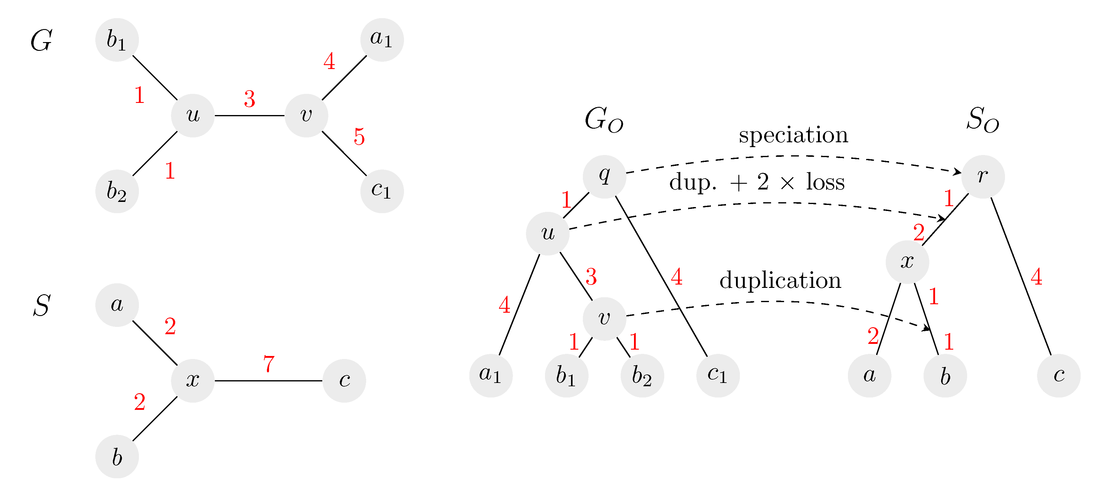
An example of an isometric reconciliation of two unrooted trees. On the left, the input gene tree G and species tree S are shown, both unrooted. On the right is one possible solution, consisting of rooted trees and and a mapping between them. The species tree is rooted on edge at distance 4 from c. Once the root of S is fixed, the rest of the solution is given uniquely. All possible roots in S are located on the edge in distances from 0 to 5 from c. Note that in our algorithm, we preprocess tree S to have two leaves and instead of leaf b, so that the leaves of G and S are in one-to-one correspondence (see Section 2.1 and Section 2.8).
Figure 2.
An example of an isometric reconciliation of two unrooted trees. On the left, the input gene tree G and species tree S are shown, both unrooted. On the right is one possible solution, consisting of rooted trees and and a mapping between them. The species tree is rooted on edge at distance 4 from c. Once the root of S is fixed, the rest of the solution is given uniquely. All possible roots in S are located on the edge in distances from 0 to 5 from c. Note that in our algorithm, we preprocess tree S to have two leaves and instead of leaf b, so that the leaves of G and S are in one-to-one correspondence (see Section 2.1 and Section 2.8).

Figure 3.
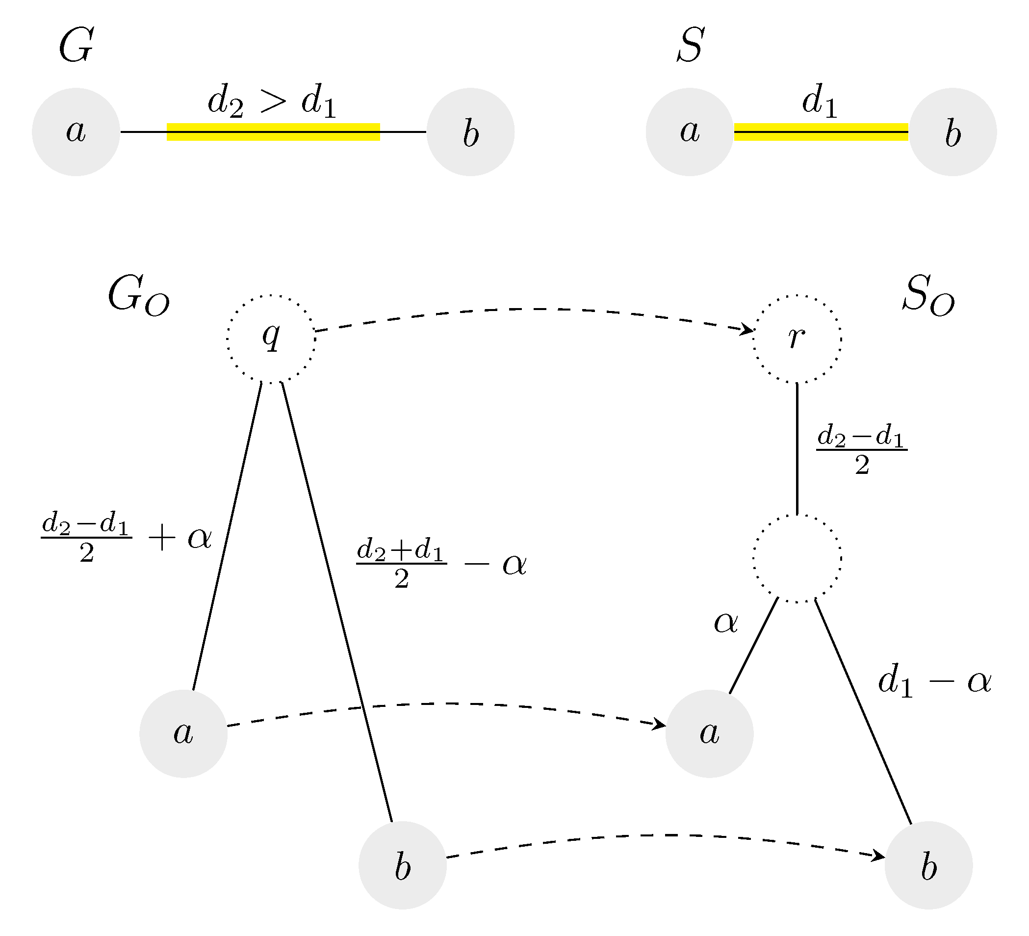
An example of two unrooted trees and their isometric reconciliation, in which the root of is mapped to a point above the original root of S. Both input trees consist of only a single edge; the length of the edge is greater in G. Tree S can be rooted in any point, while the corresponding roots of G form an interval of length in the middle of the edge. Valid roots are highlighted in yellow.
Figure 3.
An example of two unrooted trees and their isometric reconciliation, in which the root of is mapped to a point above the original root of S. Both input trees consist of only a single edge; the length of the edge is greater in G. Tree S can be rooted in any point, while the corresponding roots of G form an interval of length in the middle of the edge. Valid roots are highlighted in yellow.

Figure 4.
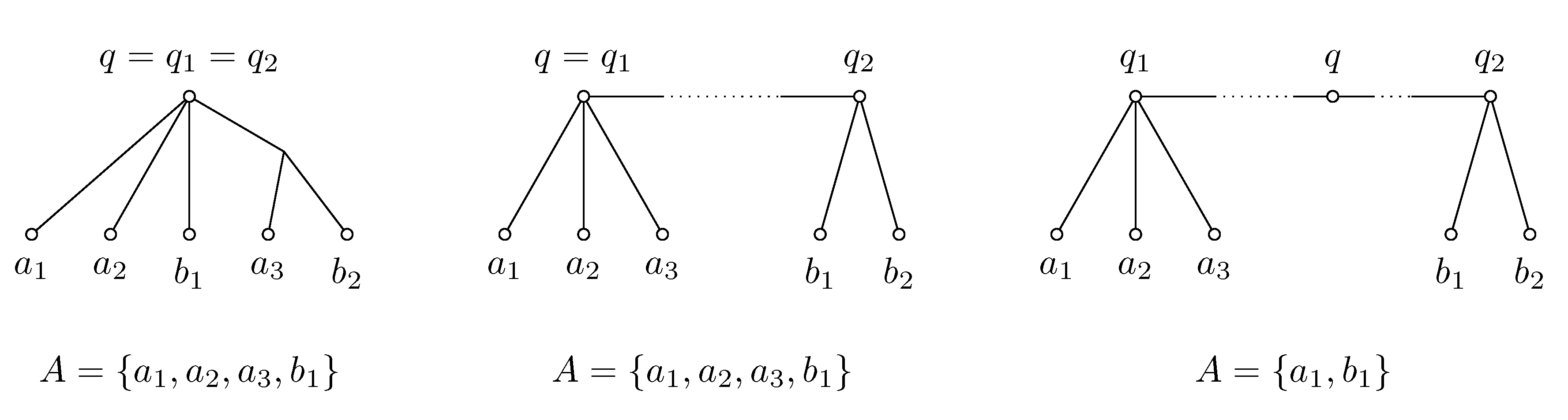
Construction of representative set A for q from representative sets and . The algorithm in the text considers three different cases depicted from left to right. Construction of set A involves some arbitrary choices; for example, in the first case, can be replaced in A by .
Figure 4.
Construction of representative set A for q from representative sets and . The algorithm in the text considers three different cases depicted from left to right. Construction of set A involves some arbitrary choices; for example, in the first case, can be replaced in A by .

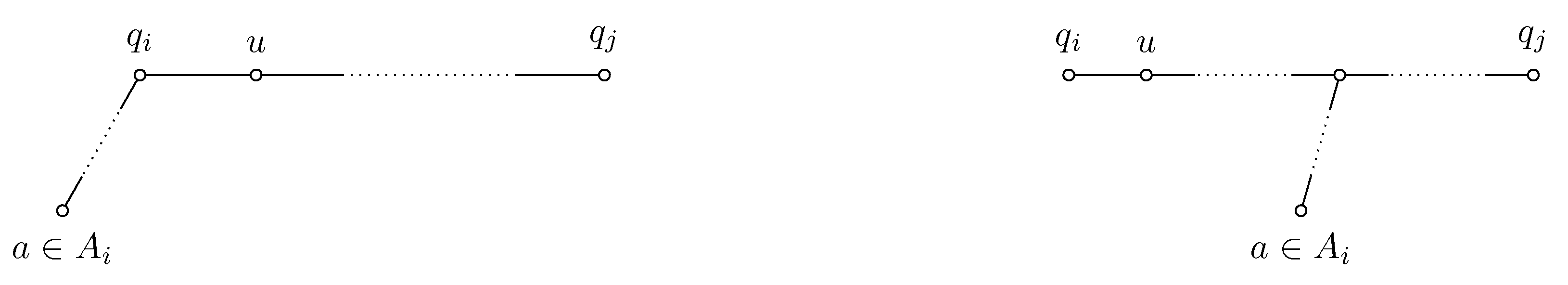
Figure 5.
Illustration of the algorithm for checking Condition 3 when . We need to check that the path connecting and is outside except for . For each leaf a from the representative set of , we check that is true. Left: is true; right: is false, .
Figure 5.
Illustration of the algorithm for checking Condition 3 when . We need to check that the path connecting and is outside except for . For each leaf a from the representative set of , we check that is true. Left: is true; right: is false, .

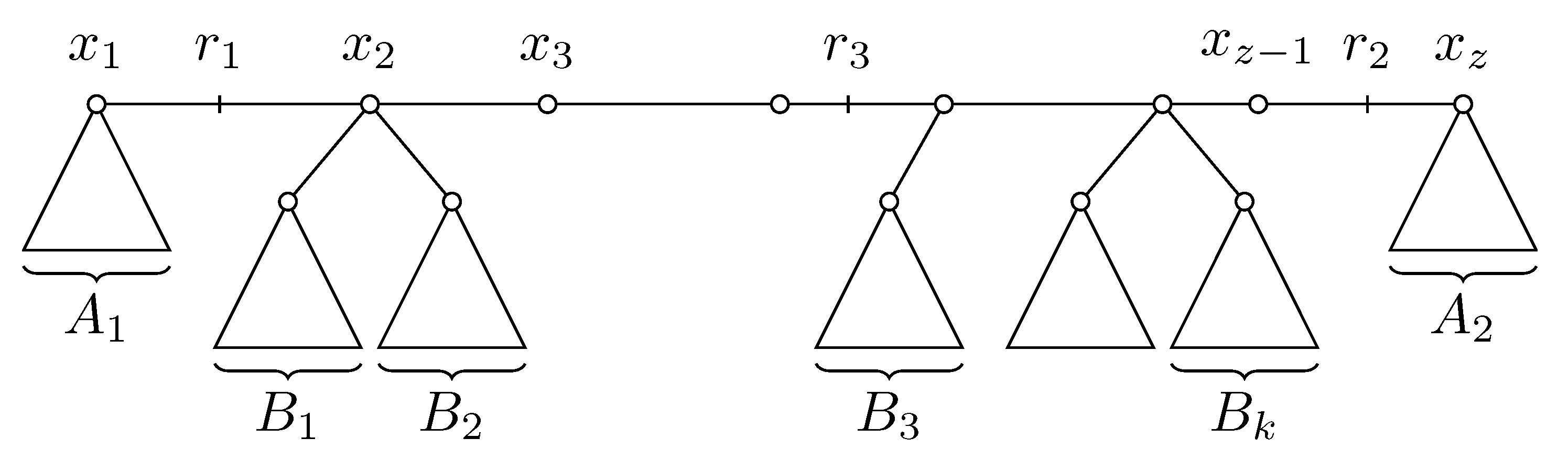
Figure 6.
The path containing , and in tree S. Leaves are partitioned into sets , and B, where B is in the figure represented by the union .
Figure 6.
The path containing , and in tree S. Leaves are partitioned into sets , and B, where B is in the figure represented by the union .

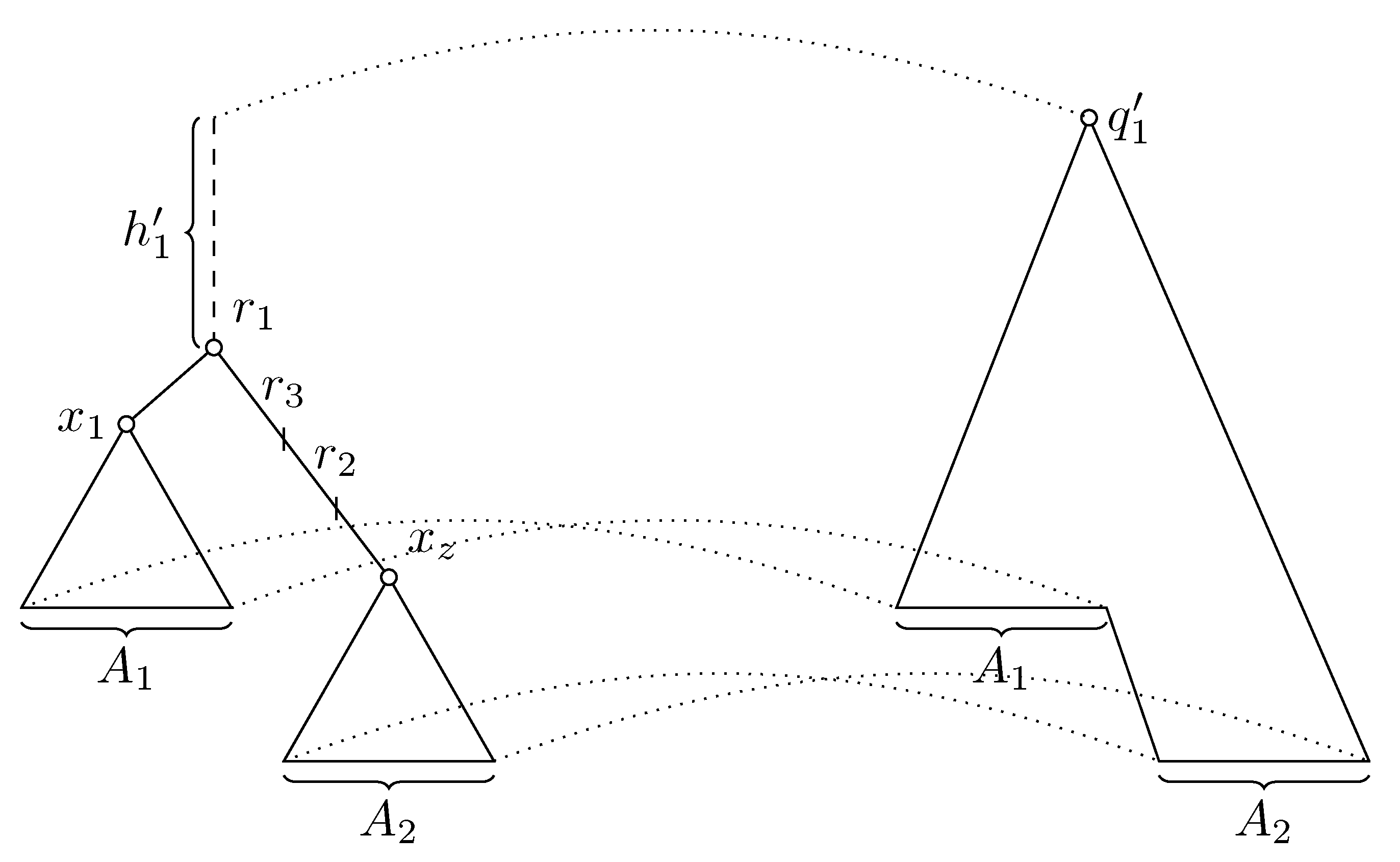
Figure 7.
Tree (left) and tree with potential rooting (right).

© 2020 by the authors. Licensee MDPI, Basel, Switzerland. This article is an open access article distributed under the terms and conditions of the Creative Commons Attribution (CC BY) license (http://creativecommons.org/licenses/by/4.0/).
Share and Cite
MDPI and ACS Style
Brejová, B.; Královič, R. A Linear-Time Algorithm for the Isometric Reconciliation of Unrooted Trees. Algorithms 2020, 13, 225. https://0-doi-org.brum.beds.ac.uk/10.3390/a13090225
AMA Style
Brejová B, Královič R. A Linear-Time Algorithm for the Isometric Reconciliation of Unrooted Trees. Algorithms. 2020; 13(9):225. https://0-doi-org.brum.beds.ac.uk/10.3390/a13090225
Chicago/Turabian StyleBrejová, Broňa, and Rastislav Královič. 2020. "A Linear-Time Algorithm for the Isometric Reconciliation of Unrooted Trees" Algorithms 13, no. 9: 225. https://0-doi-org.brum.beds.ac.uk/10.3390/a13090225
Note that from the first issue of 2016, this journal uses article numbers instead of page numbers. See further details here.