Simulated Annealing with Exploratory Sensing for Global Optimization


1
Department of Computer Sciences and Artificial Intelligence, College of Computer Sciences and Engineering, University of Jeddah, Jeddah 21589, Saudi Arabia
2
Department of Computer Science in Jamoum, Umm Al-Qura University, Makkah 25371, Saudi Arabia
3
Computers and Systems Engineering Department, Mansoura University, Mansoura 35516, Egypt
4
Department of Electrical Engineering, Computer Systems Department, Faculty of Engineering, Aswan University, Aswan 81542, Egypt
5
Department of Computer Science, Faculty of Computers & Information, Assiut University, Assiut 71526, Egypt
*
Author to whom correspondence should be addressed.
Algorithms 2020, 13(9), 230; https://0-doi-org.brum.beds.ac.uk/10.3390/a13090230
Submission received: 23 July 2020
/
Revised: 16 August 2020
/
Accepted: 10 September 2020
/
Published: 12 September 2020
Abstract
:Simulated annealing is a well-known search algorithm used with success history in many search problems. However, the random walk of the simulated annealing does not benefit from the memory of visited states, causing excessive random search with no diversification history. Unlike memory-based search algorithms such as the tabu search, the search in simulated annealing is dependent on the choice of the initial temperature to explore the search space, which has little indications of how much exploration has been carried out. The lack of exploration eye can affect the quality of the found solutions while the nature of the search in simulated annealing is mainly local. In this work, a methodology of two phases using an automatic diversification and intensification based on memory and sensing tools is proposed. The proposed method is called Simulated Annealing with Exploratory Sensing. The computational experiments show the efficiency of the proposed method in ensuring a good exploration while finding good solutions within a similar number of iterations.
1. Introduction
Metaheuristics work on finding fast and acceptable solutions for complex problems by trial and error methods. The problem complexity prevents pursuing every possible solution; therefore, the goal is to acquire a satisfactory and feasible solution within a suitable time. Theoretically, there is no guarantee to find the best solutions, and it is not recognized whether the algorithm will converge or not. Hence, design an efficient and practical algorithm that can mostly find a high-quality solution within a suitable time is crucial. In the past four decades, many applications and studies have applied Metaheuristics algorithms. tabu search (TS) [1], simulated annealing (SA) [2], genetic algorithms (GAs) [3], and other plentiful numbers of metaheuristics algorithms which have attracted much attention compared to each other.
Generally, most of the well-known metaheuristics techniques are memory-less algorithms. Memory-less means that there is no idea about the history of previously found solutions. Thus, based on memory usage, metaheuristics can be classified into algorithms with memory and memory-less ones. The absence of memory in metaheuristics leads to the loss of the information gained in previous iterations. Thus, in many cases, this leads to re-visiting the already visited areas in the search region. It is clear that without a history/memory, a new search would be done in those areas with a chance of repeating the old solution. Thus, the time consumption cost will be high. On the other hand, using memory to build a history for “some” recent solutions in the already visited areas will save the computations’ time. However, few pieces of metaheuristics research employed memory in their methods. Therefore, in the advanced metaheuristics, memory should be considered one of the fundamental elements of an efficient metaheuristic. In [4], a recent review of the memory usage and its effect on the performance of the main swarm intelligence metaheuristics. The investigation has been performed for memory, memory-less metaheuristics, and memory characteristics, especially in swarm intelligence metaheuristics. It has been investigated and shown that memory usage is essential to increase the effectiveness of metaheuristics by taking advantage of their previous successful histories.
Simulated annealing (SA) is a well-known search algorithm used successfully in many search and optimization problems. Typically, the random walk of SA does not benefit from the memory of visited states, which can cause excessive random search and redundant behavior, especially with weak configurations of the SA. Moreover, unlike memory-based search algorithms such as tabu search, the search in SA is dependent on the choice of the initial settings to explore the search space and finding an acceptable solution. At the same time, there are limited indications of how much exploration has been carried out. Also, the lack of exploration eye can affect the quality of the final solutions and the termination time, which causes practitioners to use more extended cooling and substantial initial temperatures and increase the number of iterations, especially when the minimum cost is unknown.
A few studies use different ways to overcome these issues. For example, in [5], a hybrid simulated annealing with solutions memory elements to solve university course timetable problems has been proposed. A memory-based methodology that redirects the search to return to unaccepted visited solutions when trapped in local minima has been used to escape from local minima. Authors in [6] proposed a hybrid algorithm that integrates different heuristics features, including using three types of memories, one long-term memory, two short-term memories, and an evolution-based diversification approach. In [7], a memory-based simulated annealing (MSA) algorithm is proposed for the fixed-outline floor planning of blocks. MSA implements a memory pool to keep some historical best solutions during the search. Moreover, MSA uses a real-time monitoring strategy to check whether a solution has been trapped in a local optimum. Moreover, as a solution for the slow convergence problem, an Adaptive simulated annealing genetic algorithm (ASAGA) based on a mutative scale chaos optimization strategy is proposed in [8]. The algorithm can benefit from the parallel searching structure of the GA and the probabilistic jumping property of the SA, besides implementing an adaptive crossover and mutation operators. The results proved finding the global one more quickly. In [9], an enhanced simulated annealing algorithm was developed by integrating “directional search” and “memory” capabilities. The algorithm performance is improved by directing the search based on a better understanding of the configuration space’s current neighborhood. A Tabu Search with memory concept and an enhanced annealing method is tested and improved the convergence rate and quality. A multi-objective simulated annealing (MOSA) and an adaptive memory procedure (MOAMP) is proposed in [10]. These algorithms are tested by finding a set of non-dominated solutions of hybrid flow shop scheduling problems concerning both objectives of total setup time and cost. Without memory, the simulated annealing is time-consuming and has difficulty controlling the temperature and transition number. In [11], an annealing framework with a learning memory is implemented. That proposed framework showed reasonable confidence in the solution quality. Moreover, there are several attempts to improve the SA performance through hybridization with different metaheuristics [12,13,14], or thought invoking restart strategies [15,16,17].
On the other hand, several alternative nature-inspired optimization algorithms have been proposed to deal with general global optimization problems, such as genetic algorithms [18,19,20], evolution strategies [21,22], evolutionary programming [23,24], tabu search [25], memetic algorithms [26,27,28], differential evolution [29,30,31,32], particle swarm optimization [33,34,35,36,37], scatter search [38,39], ant colony optimization [40,41,42], artificial bee colony [43,44], variable neighborhood search [45,46], and hybrid approaches [47,48,49,50,51,52]. Besides these well-known techniques, other new methods which recently proposed including multi-verse optimizer [53], fuzzy adaptive teaching [54], whale optimization algorithm [55], wolf preying behavior [56], and drone squadron optimization [57].
In this paper, we propose a two-phase methodology using automatic diversification and intensification based on memory and sensing tools in this work. Actually, one of the challenging issues in two phases hybrid algorithms is the timing of the switch between the diversification-oriented algorithm and the local-oriented search algorithm leading to the need for incorporating diversity measures [51]. Therefore, an efficient metaheuristic approach for finding a global optimum of optimization problems is presented to achieve a wide and deep search. The proposed method is called simulated annealing with exploratory sensing (SAES) that integrates different features of several well-known heuristics. The proposed algorithm’s core is a simulated annealing module that is integrated with exploration and diversification schemes to enhance the search process using adaptive search memories. In particular, a Gene Matrix (GM) concept [58,59] is constructed to sample the search space, guide the search process, and to accelerate the method termination. The GM is used as a diversification tool to record a history of space’s visited partitions. New solutions will be created in the non-visited partitions; therefore, the search process is directed to visit individuals in these partitions during the diversification process. After having the GM matrix filled with ones giving an indicator of visiting most partitions, an intensification process starts. More intensification as a local search in its region will be carried out from the best-found solution. Finally, a faster local search is applied to help the SA algorithm quickly target optimal solutions. This could improve the search process outputs since the SA-based algorithm is known to be reel around optimal solutions in the final stages of the search. Numerical results of the proposed SAES method verify that the designed procedures and memory elements are efficient, and the proposed methods are competitive with some other types of benchmark methods.
In the rest of this paper, we discuss the related works of the SA module and the concept of sensing search memory in Section 2. Then, our proposed method SAES with sensing memories and operations is presented in Section 3. The numerical simulations are presented and discussed in Section 4. Finally, Section 5 shows concluding remarks.
2. Simulated Annealing and Sensing Memory
In this section, the structure of the simulated annealing algorithm is sketched, and the main concept of the sensing search memory is highlighted.
2.1. Simulated Annealing Algorithm
Annealing theory is based on condensed matter physics, where particles in a physical system control the behaviors of the annealing process [2]. Simulated annealing implements the Metropolis algorithm to emulate metal annealing in metallurgy, where heating and controlled cooling reshape the metal particles. Controlling the metal temperature carefully by increasing it to higher values and decreasing it arranges the particles to minimize the system energy. The standard SA algorithm is a successful randomized local search algorithm for finding minima or near minima solutions of optimization problems [60]. It is a particularly valuable tool for solving high dimensionality problems [61]. Although the SA method can find solutions for extensive range problems, its main drawback is the high computational time [60].
Let s be the current state and alternative states in its neighborhood . One state is selected, and the difference between the current state cost and the selected state energy is computed as . Metropolis criterion is used to choose as the current state in two cases:
- If , means the new state has a smaller or equal cost, then is chosen as the current state as down-hills is always accepted.
- If , and the probability of accepting is larger than a random value such that then is chosen as the current state where T is a control parameter known as . This parameter is gradually decreased during the search process, making the algorithm greedier as the probability of accepting uphill moves decreases over time. Moreover, is a randomly generated number, where . Accepting uphill moves is important for the algorithm to avoid being stuck in local minima.
In the last case where and the probability is lower than the random value , no moves are accepted, and the current state s continues to be the current solution. When starting with a large cooling parameter, large deterioration can be accepted. Then, as the temperature decreases, only small deterioration are accepted until the temperature approaches zero when no deterioration is accepted. Therefore, adequate temperature scheduling is essential to optimize the search. SA can be implemented to find the closest possible optimal value within a finite time where the cooling schedule can be specified by four components [60]:
- Initial value of temperature.
- A function to decrease temperature value gradually.
- A final temperature value.
- The length of each homogeneous Markov chains. A Markov chain is a sequence of trials where the trial outcome’s probability only depends on the previous trial outcome. It is classified as homogeneous when the transition probabilities do not depend on the trial number [62].
The success of SA depends on how good the choice of its parameters. For instance, the algorithm can be stuck in a local minimum when choosing small initial temperatures since the exploration process must be carried during the first stages. On the other hand, a significant temperature could cause the convergence to be very slow. The same effect can be obtained when applying an inappropriate cooling schedule. Also, adjusting the neighborhood range for SA is essential in continuous optimization problems [63]. All inputs should not have the same step sizes, but these steps should be selected according to their effects on the objective function [64]. The authors in [65] proposed a method to identify the step size during the annealing process, which begins at significant steps and gradually decreases them. The initial temperature can also be chosen within the standard deviation of the mean cost of several moves [66]. When finite Markov chains are used to model SA mathematically, the temperature is reduced once for each Markov chain. In contrast, each chain’s length should be related to the size of the neighborhood in the problem [60].
2.2. Sensing Search Memory
An adaptive data storage called the sensing search memories is constructed to collect the search data to boost the search process. There are various types of sensing search memories, such as Gene Matrix (GM) and Landmarks Matrix (LM) [22,23,58,59]. These memories can be invoked by collecting data and solution features from different and diverse search space regions. The following GM, as a sensing search memory, is applied in this research.
Gene Matrix (GM)
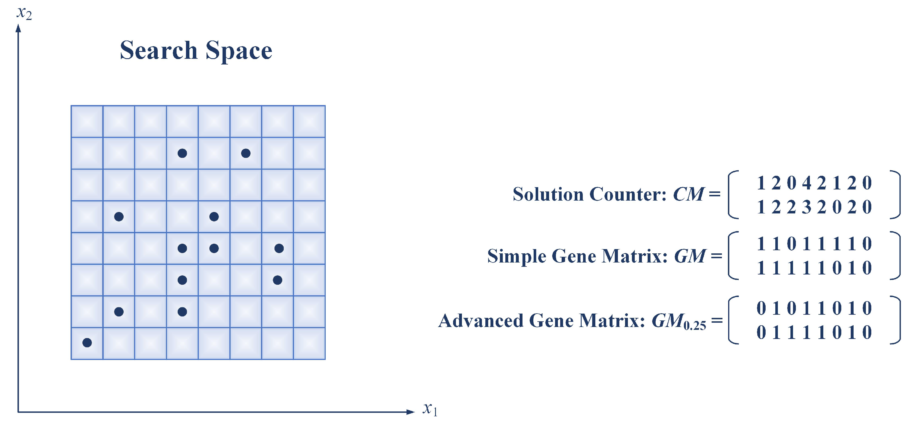
The GM sensing search memory collects data and features from different and diverse search space regions. The GM memory is invoked to assess the exploration process during the search. The search methods use different coding representations of individuals, which applies every solution x in the search domain to comprise n variables or genes. Specifically, in the GM, each variable range is divided into m sub-range. Then, each sub-range of the i-th gene is associated with the entry of the i-th row of the gene matrix. Therefore, the GM memory is initially an zero matrix. Then it is converted to ones whenever the corresponding sub-ranges are visited during the search process.
The update process of the GM entries from 0 to 1 is controlled with a parameter to ensure that each sub-range is visited at least times. As an example of the GM, Figure 1 shows a 2-dimension GM with . The range of each gene in this example is split into 8 sub-ranges. Two GM are defined; a simple GM which requires only one visit to update its entities from 0 to 1, and the advanced GM that requires at least visits to update its entities. Therefore, both of the GM and GM have zero entities at the third and eighth sub-ranges of gene since no individual has been generated in these sub-ranges. However, entry in GM is equal to 0 as there exists only one individual in the third sub-range. The entry can be updated to 1 if one extra individual has been generated in the consequent generations.
The GM is an indicator of an advanced exploration process when there is no zero elements in the GM, and the search process can be terminated. Consequently, the GM is used to provide the search process with reasonable termination criteria. Furthermore, diverse solutions will be afforded to the search space, as will be explained later.
3. Simulated Annealing with Exploratory Sensing (SAES) Algorithm
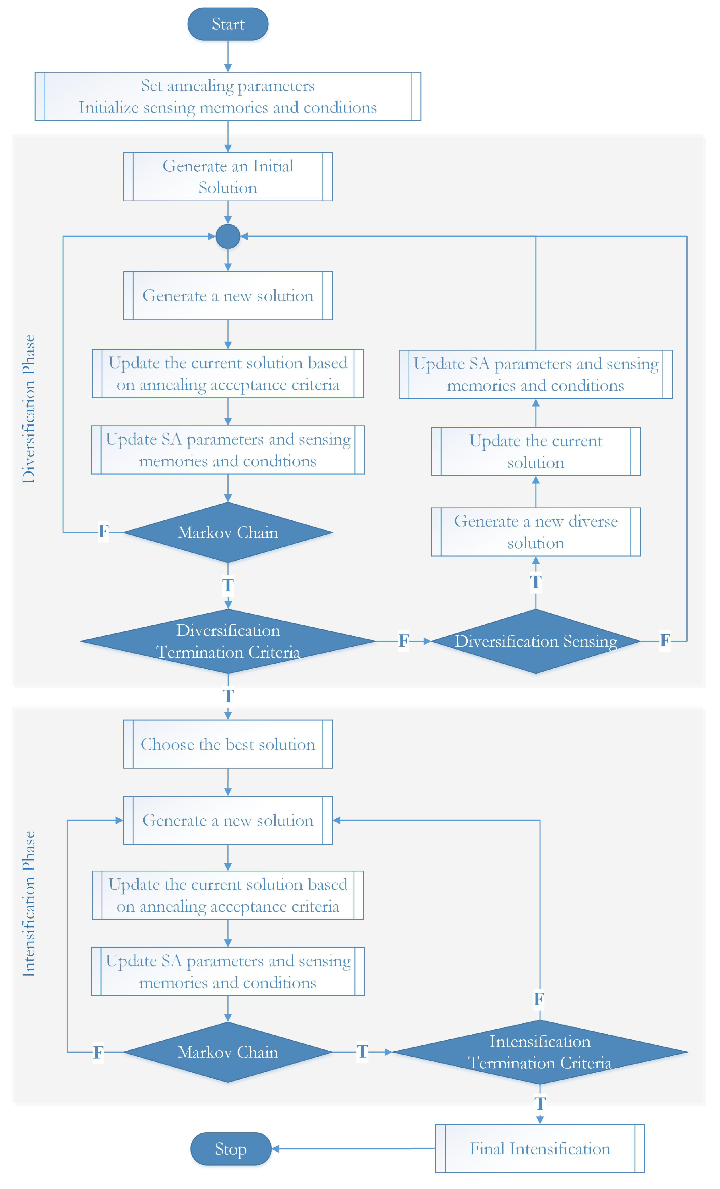
The objective of the proposed work is to increase the probability of finding a global optimum by using a memory-based mechanism. The GM works as a sensing search memory where the visited partitions are recorded to ensure the exploration of the search space. The search walker is then enforced to attend non-visited partitions after several iterations (Markov chains) while keeping a record of several best solutions found, as shown in the flowchart in Figure 2. Also, the search is carried out in two phases:
- (1)
- The exploration phase. This stage has several iterations within several Markov chains and aims to explore the constrained search space within the lower and upper limits of the solutions’ values without affecting the way of how SA works in each Markov chain. Instead of starting the new Markov chain from the last accepted state, applying the GM directs the search to visit solutions in non-visited partitions of the search space. The cooling schedules and the acceptance criteria are not affected by applying the GM, while the temperature is changed in each Markov chain ones. Therefore, in each Markov chain, an intensification process is carried out in the new partition of the search space, while the search is keeping records of the best-found solutions.The adjustment of the SA settings should explore the search space in the first phase. Extensive exploration is maintained in our proposed method by a diversification index. The diversification index is a ratio of the number of visited partitions to the number of all partitions in the GM, and it is measured after each Markov chain. For instance, this phase can be ended when the diversification index reaches a pre-defined ratio of the partitions have been visited. The numerical experiments shown later indicate that the appropriate value for the parameter is , and this means visiting a percentage greater than of the GM partitions. Another parameter called a diversification threshold is applied to control the direction to un-visited partitions of the search space and this is called diversification sensing. This parameter is a smaller anticipated value of the diversification index. For example, the diversification threshold value , means that when the search in one Markov chain has not changed the diversification value by this threshold, the diversification process will be called to move to new search partitions. Otherwise, the diversification process is not used as the search is achieving good diversification using the escaping mechanism.
- (2)
- The intensification phase. After reaching a specified level of diversification where most of the searching partitions were visited, the search is directed to start from the best-found state to do a more local search in that region. Although the diversification is supposed to be achieved mainly in the first phase using the GM, it is essential to ensure that the initial temperature is wisely chosen to avoid getting trapped in local minima earlier at the start of this phase. We choose to use a static cooling schedule that allows sufficient temperature after ending the exploration phase. The search is ended when reaching the maximum iteration, which equals the number of Markov chains multiplied by each Markov chain’s length.
After the two leading search phases are accomplished, a faster local search is called to refine the best solution obtained so far. This could improve the SA algorithm output since this algorithm is known to be reel around optimal solutions in the final stages of the search [67,68]. It is worth noting that the two phases are executed sequentially and not overlapping together to maintain the main structure of the SA algorithm, especially the cooling scheduling. This is also so that the proposed algorithm does not lose the convergence behavior recognized in the standard SA algorithm.
The components of the proposed algorithm are presented and explained in the following subsections.
3.1. Neighborhood Representation
The neighborhood representation is defined by moving one or more of these parameters to one or more directions randomly by a defined move class, e.g., by adding a defined step size to one or more of the current parameter’s values to a specific direction. One move class is randomly choosing neighboring solutions for a current solution by generating new solutions based on the current solution. This generation process uses a multivariate normal distribution with step sizes equal to the square root of the temperature and uniformly random direction. This choice is known as a typical choice for generating new solutions in SA as noted by [69]. In addition, the initial temperature is set as the standard deviation of different random moves, as presented by [66], this leads to a temperature value related to the size of inputs. Therefore, this is a good choice when testing tens of different problems with different scales to avoid the problem of small or large step sizes that can badly affect the search convergence. Each time a new solution is generated, the boundary conditions are checked, and new bounded values are generated when needed. Then, the cost of the new state is evaluated.
3.2. Initial Solution
Simulated annealing requires an initial solution. Typically, the SA performance highly dependents on the initial solution settings, especially with relatively small temperatures or fast cooling schedules. Alternatively, our methodology is not affected by the initial solution values as the diversification process should overcome the initial settings traps. Specifically, the quality of the initial solution does not affect the quality of the obtained solutions due to the proposed diversification mechanism that redirects the search after each Markov chain of iterations into new areas rather than digging in promising areas. Actually, the proposed methodology concerns with increasing intelligent coverage of the visited solutions and exploiting search memory through the proposed diversification. Therefore, a random initial solution is selected in implementing the SAES method.
3.3. Objective Function
The objective function is defined for each benchmark function, as shown in Appendix A and Appendix B. In general, we concern with the following global optimization problem:
where f is a real-valued function defined on search space .
3.4. Initial Temperature Settings
Setting appropriate initial temperature and cooling schedule is crucial for having an efficient SA method. The initial temperature is set as the standard deviation of 100 random moves, as presented by [66].
Cooling Schedule
An appropriate cooling schedule is important for the success of the SA algorithm as fast cooling can cause the algorithm to become stuck in a local minimum, and slow cooling can make the convergence very slow. A suitable static or dynamic cooling rate will help the SA converge to a global minimum and avoid getting stuck in a local minimum. We choose the static cooling schedule:
where is a static cooling rate. Setting close to 1 allows more exploration for the search space, while smaller setting values allow greedier search and might not explore the whole search space inside each Markov chain. Normally, practitioners use a static cooling rate between 0.8–0.99 [60]. The cooling schedule used is based on Boltzmann annealing by updating each iteration’s current temperature based on the initial temperature and the current iteration number .
3.5. Markov Chains Configurations
When using Markov chains to model the SA iterations mathematically, the temperature is reduced once for each Markov chain. The number of Markov chains chosen for this experiment is 60 chains, which we think is enough for this study. The length of each chain should be related to the size of the neighborhood in the problem [60]. Our case’s neighborhood size is the number of all optimized parameters involved in the optimization process multiplied by 40.
3.6. The Diversification and Intensification Settings
A matrix of search space partitions called Gene Matrix GM is used. The SA algorithm uses the real-coding representation of individuals, which applies individual x in the search space to comprise n variables or genes. Every gene’s scope is split into m sub-ranges to check the diversity of the gene values. At that point, a solution counter matrix C of size is built, in which term stands for the number of produced solutions such that gene i lies in the sub-range j, where , and . In the initialization stage, the GM is built to be a zero matrix in which every entry of the i-th raw indicates a sub-range of the i-th gene. During the search phase, the GM zero values will be flipped to ones when new values are created in corresponding sub-ranges. The GM is an indicator of an advanced exploration process when there is no zero entry in the GM, and the search process can be terminated. Consequently, GM is used to provide the search process with reasonable termination criteria. The diversification threshold is chosen to be , where diversification is not called if the algorithm achieved diversification improvement upper than this threshold in the exploration phase. Diversification stops when stopping criteria is observed by one of two conditions. The first is when reaching the diversification index of , which implies 90% of the number of partitions have been visited. The second case when finishing of the number of Markov chain iterations.
3.7. Stopping Criterion
Typical stopping criteria of the SA includes stopping at small objective function values, stopping at lower temperature values, stopping after sufficient iterations or Markov chains, and stopping when the changes of energy in the objective function are sufficiently small. The choice of stopping criterion is difficult as the optimal objective function is unknown in many cases [70]. When using any stopping criteria, the objective of the two phases might be watched in which the diversification and the intensification objectives should be achieved. To get good results, we have chosen to stop the search after a certain number of Markov chains represent of the number of all Markov chains.
3.8. The SAES Algorithm
Based on the previously explained components, the whole structure of the SAES method and the sequence of its steps are illustrated in Algorithm 1.
| Algorithm 1 SAES |
|
4. Numerical Simulation
In the section, the implementation setting and experimental results are discussed. The proposed algorithm is programmed using MATLAB. The parameter setting and performance analysis of the SAES are first investigated before presenting the results and comparisons.
4.1. Test Functions
Two classes of benchmark test functions have been used in the experimental results to discuss the efficiency of the proposed methods. The first class of benchmark functions contains 25 classical test functions – [71]. Those functions definitions are given in Appendix A. The other class of benchmark functions contains 25 hard test functions – [72,73] which are known as CEC2005 test functions and described in Appendix B.
4.2. Parameter Setting and Configuration
The parameters values used in SAES algorithm are set based on the typical setting in the literature, or determined through our preliminary numerical experiments, as shown in Table 1. Based on the configuration of the SAES control parameters, there are three SA-based versions:
- The SAES without the diversification phase and final intensification, which is the standard annealing algorithm and denoted by the SA method.
- The SAES without the final intensification, which is denoted by SAES.
- The complete SAES method.
In Table 1, there are two groups of parameters. The first one in the common parameter setting, which is used in all versions of the proposed method. The other group of parameters is used in the SAES and SAES versions, except the final intensification budget is only used in the later version.
Based on the parameter values shown in Table 1, the cost of the objective function evaluations used in the SAES method can be computed as:
- Function evaluations in the initialization: 100 function evaluations.
- Function evaluations in the diversification phase: , where is the number of Markov chains in the diversification phase, which is at maximum 18.
- Function evaluations in the diversification phase: .
- Function evaluations in the final intensification: at maximum .
Therefore, the total number of function evaluations used by the SAES method is bounded by functions evaluations. Likewise, it can be concluded that these numbers in the SA and SAES versions are bounded by and , respectively.
The local search method used in the final intensification is consists of applying the MATLAB functions “fminsearch.m” and “fminunc.m” starting from the best solutions obtained in the previous search stages. Specifically, the function “fminsearch.m” is first called with the half of the local search budget, then the other MATLAB function is called to improve the output of the first one with the same budget as recommended in [74,75].
4.3. Statistical Tests
The non-parametric Wilcoxon rank-sum method [76,77,78,79,80] is used for determining the statistical differences between the comparative methods. The following statistical terms are used:
- The positive and negative ranks:where is the difference between the ranks of the corresponding results of the compared methods, and
- the p-value.
Besides these statistical measures, we add the measure “No. of Beats”, which contains two numbers. The first number is related to how often the first method has better results than the other method. Although the other number indicates the number of times, the second method has prevailed over the first method.
4.4. Results and Discussion
The proposed method was applied to 50 benchmark problems shown with their details in Appendix A and Appendix B. The results of the proposed SA versions are compared to each other to analyze their performance. Moreover, the SAES results are also compared to those of other benchmark methods to assess the proposed method’s efficiency.
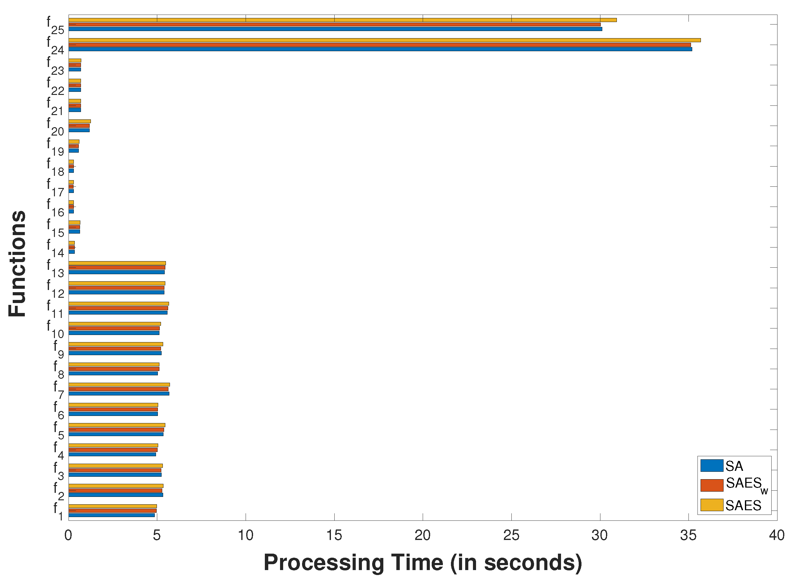
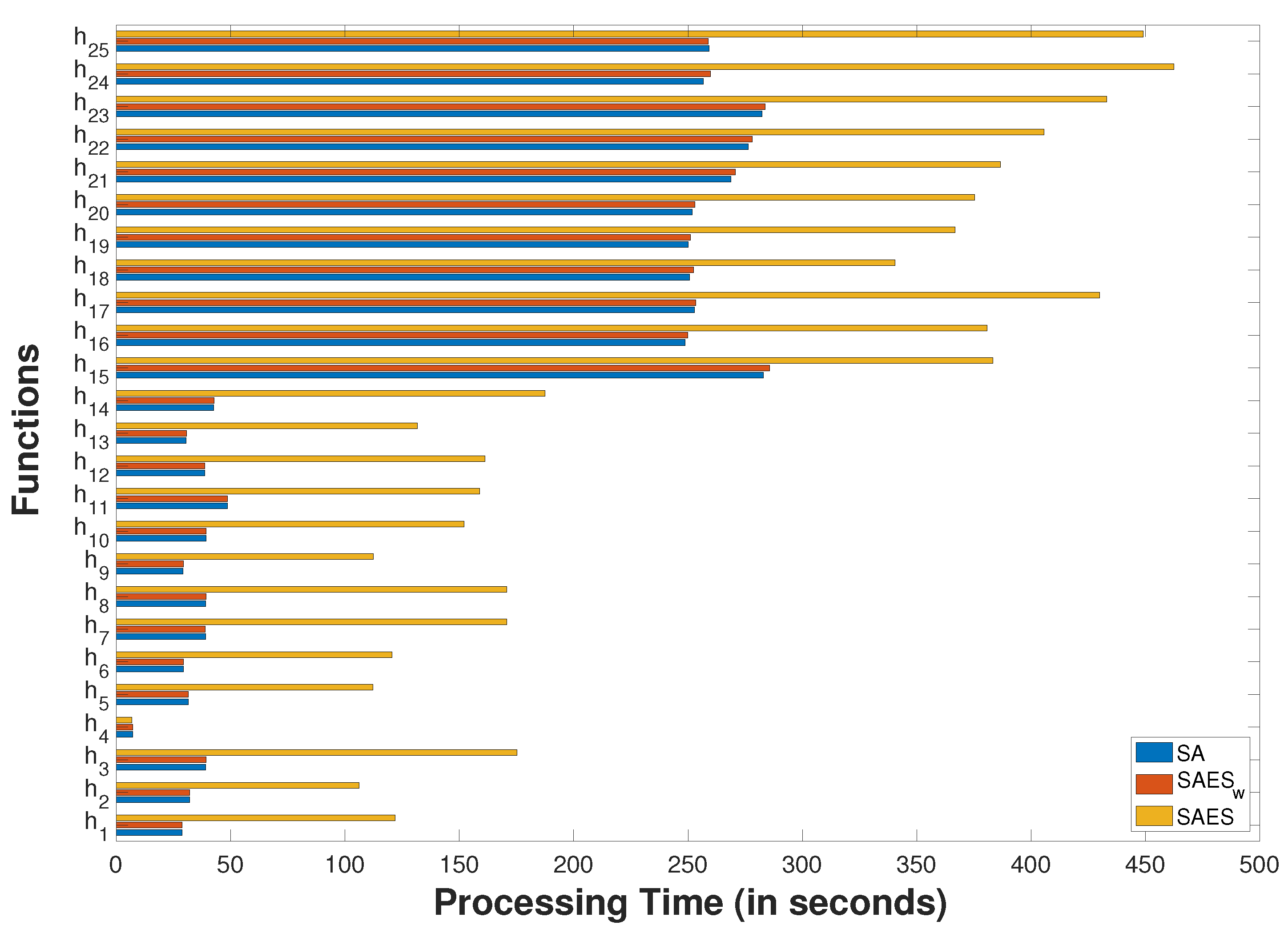
In the first experiment, the SA, SAES, and SAES methods are reported in Table 2 and Table 3 which include the averages and minima of the best solutions obtained by each method using the classical and hard test functions, respectively. The numbers of variables in classical functions − and all hard functions are set equal to 30 in this experiment. The numbers of variables in and are 100. The other functions have different numbers of variables, as shown in Appendix A. These results are recorded using 25 independent runs. The average errors between the obtained solutions shown in Table 2 and Table 3, and the global optima are reported in Table 4. Moreover, the averages of the processing time used by each method are illustrated in Figure 3 and Figure 4 using the classical and hard test functions, respectively. All these results are statistical analyzed in Table 5 and Table 6. In general, the results are improved according to the complication of the algorithm. Therefore, the results of the SAES method are better than those of the SA method and the results of the SAES is better than those of the other two methods as shown in Table 2, Table 3 and Table 4. This proves the efficiency of the main two additive components of the diversification phase and the final intensification. The processing time varies according to the problem dimension and the sophistication of the objective function formula, as shown in Figure 3 and Figure 4. The statistical measures in Table 5 and Table 6 indicate the following conclusion:
- There are no significant differences between the obtained errors in the SA and SAES methods, although the latter method could beat the first method in almost all used test functions.
- The SAES is significantly better than the other two methods in terms of obtaining better errors.
- The processing time of the SAES method is slightly longer than that of the SA and SAES methods with no significant differences between all methods processing times except in the hard test functions.
As a final note on analyzing the SAES performance in terms of its ability to reach optimal solutions, this has been studied using the relative error gap in the following formula:
where is the exact global solution, and the average solution obtained by the SAES method. The method could reach the global solutions within a gap of for 8 of the classical test functions and 3 of the hard test functions. If we consider a gap of 1, the SAES hits the vicinity of the global solutions for 11 of the classical test functions and 11 of the hard test functions. The standard SA fails to reach near global solutions for any of the classical functions or the hard functions considering the gap of or even of 1.
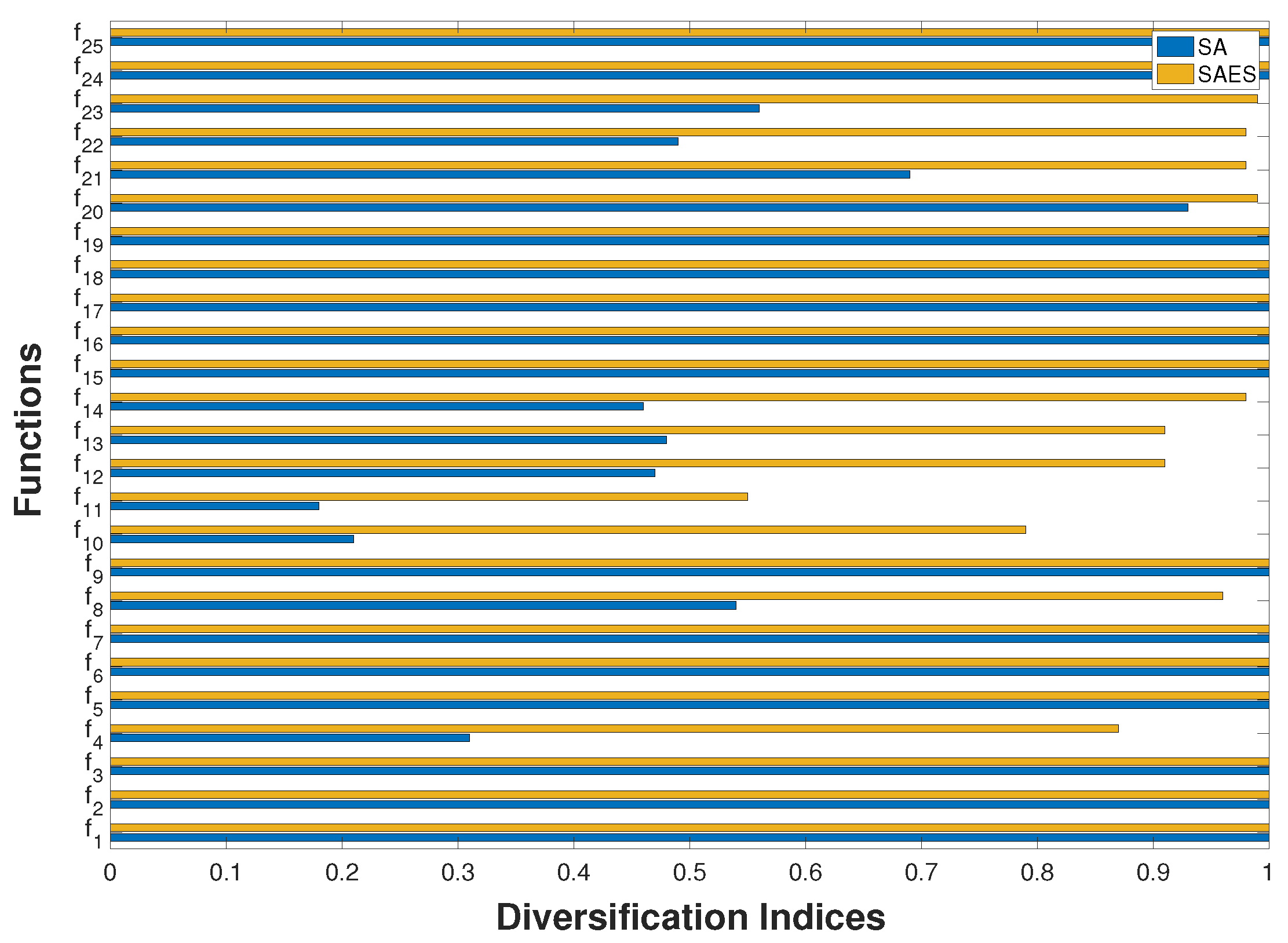
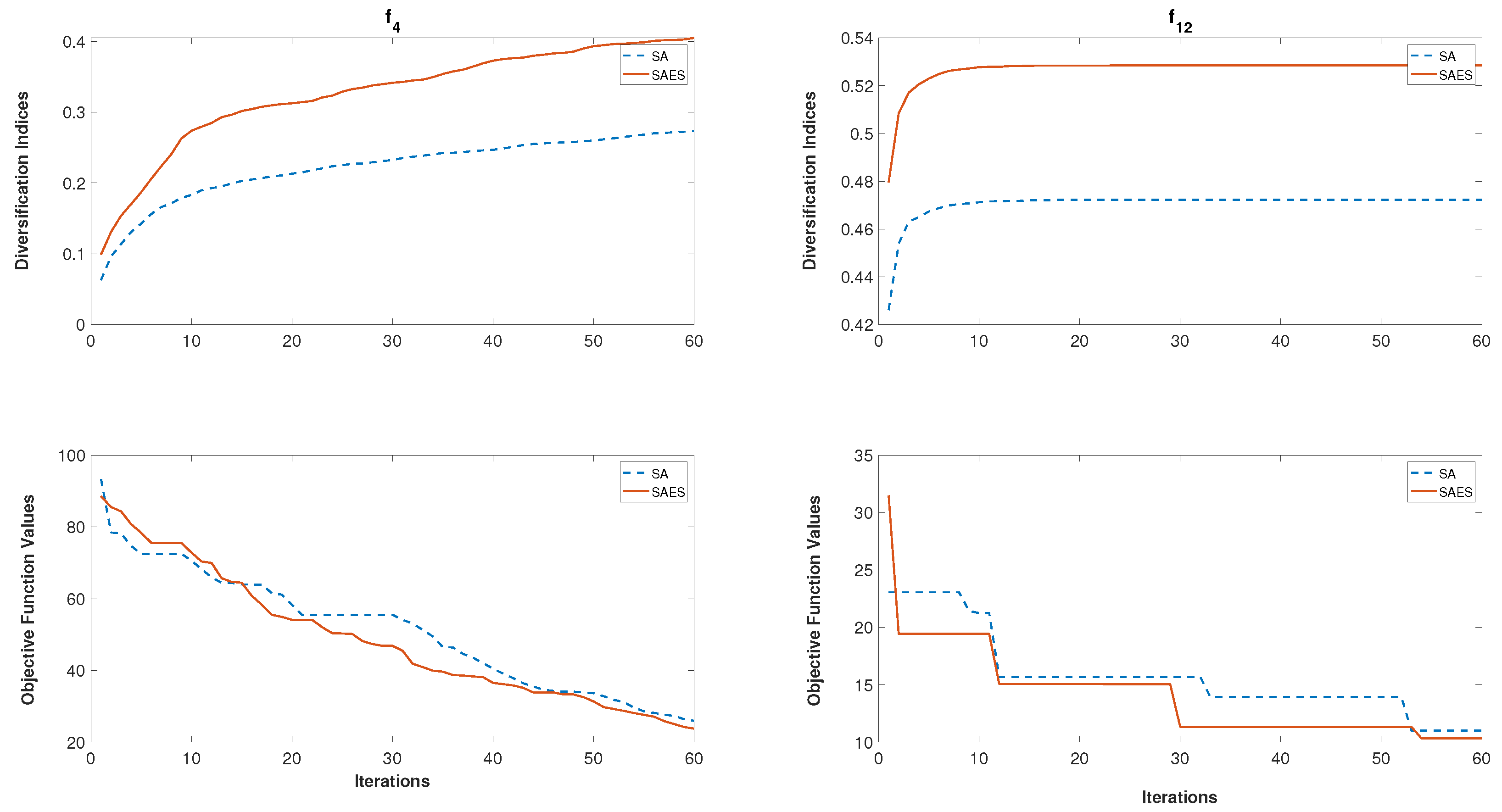
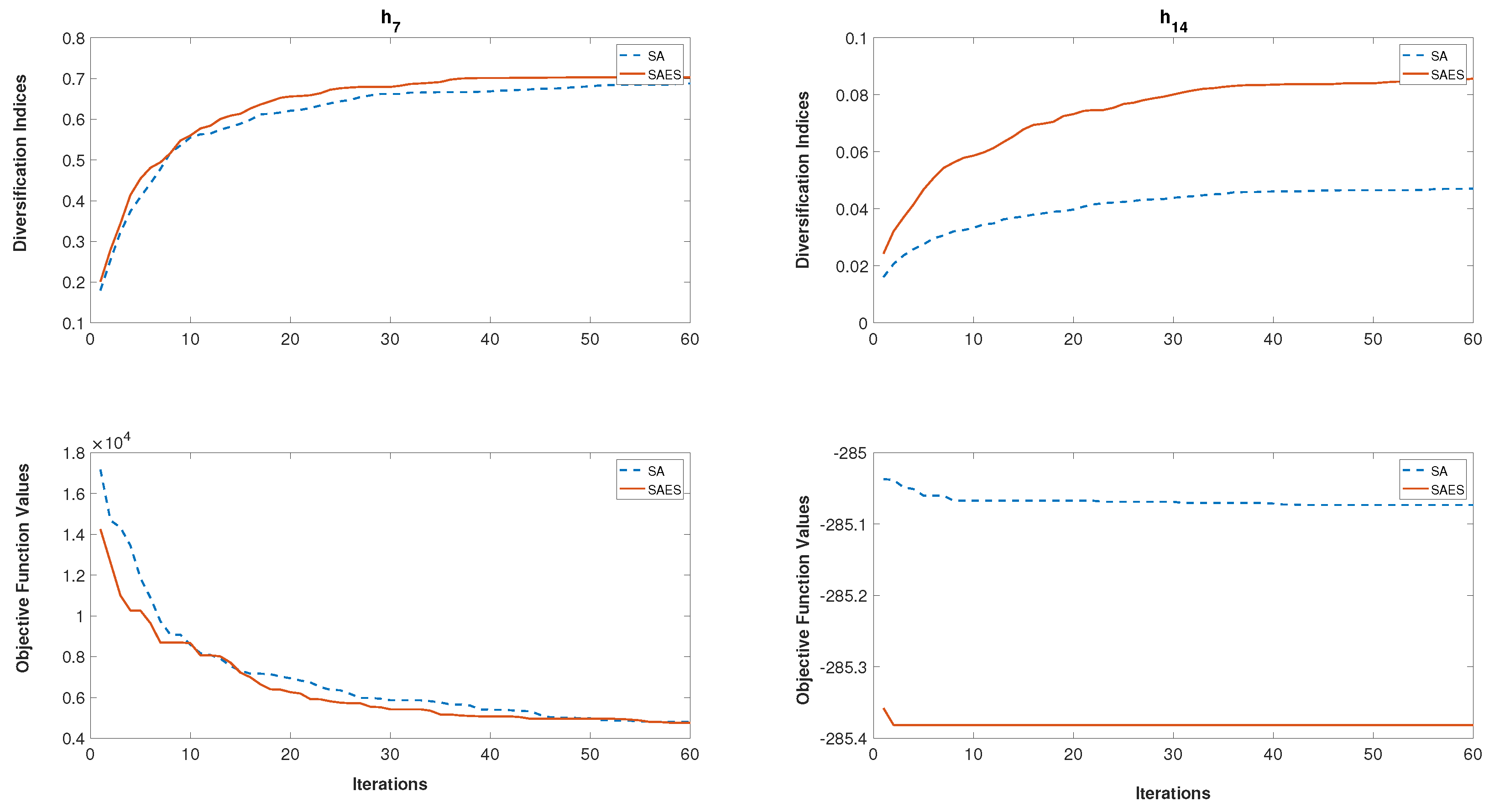
In the second experiment, we investigate the diversification index’s performance and how it could help the SA-based algorithms gain better performance. The average values of this index are reported in Figure 5 and Figure 6 over 25 independent runs using the classical and hard test functions, respectively, with the same conditions stated in the first experiment. In most of the used test functions, the diversification phase could help the SA-based algorithms explore the search space more broadly. Figure 7 and Figure 8 show examples of the progress of the best solution and diversification index improvements over generations. This shows how the diversification phase has improved the quality of obtained solutions by an SA-based method.
In the last experiment, we compare the proposed SAES with the other state-of-the-art methods abbreviated as follows, where 14 of comparative methods are used.
- BLX-GL50 [81]: Hybrid real-coded genetic algorithms with female and male differentiation.
- BLX-MA [82]: Adaptive local search parameters for real-coded memetic algorithms.
- COEVO [83]: Real-parameter optimization using the mutation step co-evolution.
- DE [84]: Real-parameter optimization with differential evolution.
- DMS-L-PSO [85]: Dynamic multi-swarm particle swarm optimizer with local search.
- EDA [86]: A simple continuous estimated distribution algorithm.
- IPOP-CMA-ES [87]: Restart with increasing population size Covariance Matrix Adaptation Evolution Strategy (CMA-ES).
- LR-CMA-ES [88]: Local restart CMA-ES.
- K-PCX [89]: A population-based, steady-state procedure for real-parameter optimization.
- L-SaDE [90]: Self-adaptive differential evolution algorithm.
- SPC-PNX [91]: Scaled probabilistic crowding genetic algorithm with parent centric normal crossover.
- cHS [92]: Cellular harmony search algorithm.
- HC [93]: Hill climbing.
- HC [94]: -Hill climbing.
The results of the benchmark mentioned above methods are reported in Table 7 along with the SAES results using the hard test functions with The results of the compared methods are taken from reference [94] with termination criteria of reaching 100,000 function evaluations while the SAES method only spends at maximum 29,118 function evaluations. The statistical measures of these results are reported in Table 8. The proposed method could beat all the compared methods in terms of function evaluations. Moreover, it shows promising competitive performance in obtaining better solutions compared with other methods used in comparisons.
5. Conclusions
A two-phase approach using automated diversification and intensification based on memory and sensing methods is suggested to enhance the SA methodology. The proposed mechanisms could enhance SA with an exploration eye that guides the search process to have better solutions. Moreover, the random walk of the standard SA algorithm has been modified to benefit from the memory of visited states and diversification history. Finally, an advanced local search can help the SA algorithm quickly target optimal solutions in the later search stages. The numerical experiments show the efficiency of the proposed method in ensuring good discovery and finding better solutions.
Author Contributions
Conceptualization, A.-R.H., H.H.A., M.A., and W.D.; methodology, A.-R.H., W.D., H.H.A. and M.A.; programming and implementation, A.-R.H., W.D. and M.A.; writing—original draft preparation, A.-R.H., W.D., H.H.A. and M.A.; writing—review and editing, A.-R.H., W.D., H.H.A., and M.A.; funding acquisition, A.-R.H. All authors have read and agreed to the published version of the manuscript.
Funding
This work was funded by the National Plan for Science, Technology, and Innovation (MAARIFAH)–King Abdulaziz City for Science and Technology–the Kingdom of Saudi Arabia, award number (13-INF544-10).
Acknowledgments
The authors would like to thank King Abdulaziz City for Science and Technology—the Kingdom of Saudi Arabia, for supporting the project number (13-INF544-10).
Conflicts of Interest
The authors declare no conflict of interest.
Appendix A. Classical Test Functions
Appendix A.1. Sphere Function (f 1)
Definition A1.
Search space:
Global minimum:
Appendix A.2. Schwefel Function (f 2)
Definition A2.
Search space:
Global minimum:
Appendix A.3. Schwefel Function (f 3)
Definition A3.
Search space:
Global minimum:
Appendix A.4. Schwefel Function (f 4)
Definition A4.
Search space:
Global minimum:
Appendix A.5. Rosenbrock Function (f 5)
Definition A5.
Search space:
Global minimum:
Appendix A.6. Step Function (f 6)
Definition A6.
Search space:
Global minimum:
Appendix A.7. Quadratic Function with Noise (f 7)
Definition A7.
Search space:
Global minimum:
Appendix A.8. Schwefel Functions (f 8)
Definition A8.
Search space:
Global minimum:
Appendix A.9. Rastrigin Function (f 9)
Definition A9.
Search space:
Global minimum:
Appendix A.10. Ackley Function (f 10)
Definition A10.
Search space:
Global minimum:
Appendix A.11. Griewank Function (f 11)
Definition A11.
Search space:
Global minimum:
Appendix A.12. Levy Functions (f 12, f 13)
Definition A12.
Search space:
Global minimum: ,
Appendix A.13. Shekel Foxholes Function (f 14)
Definition A13.
Search space:
Global minimum:
Appendix A.14. Kowalik Function (f 15)
Definition A14.
,
.
Search space:
Global minimum:
Appendix A.15. Hump Function (f 16)
Definition A15.
Search space:
Global minima: , ;
Appendix A.16. Branin RCOS Function (f 17)
Definition A16.
Search space:
Global minima: , ,
Appendix A.17. Goldstein & Price Function (f 18)
Definition A17.
Search space:
Global minimum:
Appendix A.18. Hartmann Function (f 19)
Definition A18.
,
Search space:
Global minimum:
Appendix A.19. Hartmann Function (f 20)
Definition A19.
,
.
Search space:
Global minimum:
Appendix A.20. Shekel Functions (f 21, f 22, f 23)
Definition A20.
where
.
Search space:
Global minimum:
Appendix A.21. Function (f 24)
Definition A21.
Search space:
Global minimum: .
Appendix A.22. Function (f 25)
Definition A22.
Search space:
Global minimum: .
Appendix B. Hard Test Functions
For the hard test functions -, their global minima and the bounds on the variables are listed in Table A1. For more details about these functions, the reader is referred to [72].

Table A1.
Benchmark hard functions.
| h | Function Name | Bounds | Global Minimum |
|---|---|---|---|
| Shifted Sphere | [−100,100] | −450 | |
| Shifted Schwefel’s 1.2 | [−100,100] | −450 | |
| Shifted rotated high conditioned elliptic | [−100,100] | −450 | |
| Shifted Schwefel’s 1.2 with noise in fitness | [−100,100] | −450 | |
| Schwefel’s 2.6 with global optimum on bounds | [−100,100] | −310 | |
| Shifted Rosenbrock’s | [−100,100] | 390 | |
| Shifted rotated Griewank’s without bounds | [0,600] | −180 | |
| Shifted rotated Ackley’s with global optimum on bounds | [−32,32] | −140 | |
| Shifted Rastrigin’s | [−5,5] | −330 | |
| Shifted rotated Rastrigin’s | [−5,5] | −330 | |
| Shifted rotated Weierstrass | [−0.5,0.5] | 90 | |
| Schwefel’s 2.13 | [−100,100] | −460 | |
| Expanded extended Griewank’s + Rosenbrock’s | [−3,1] | −130 | |
| Expanded rotated extended Scaffe’s | [−100,100] | −300 | |
| Hybrid composition 1 | [−5,5] | 120 | |
| Rotated hybrid comp. | [−5,5] | 120 | |
| Rotated hybrid comp. Fn 1 with noise in fitness | [−5,5] | 120 | |
| Rotated hybrid composition function | 10 | ||
| Rotated hybrid composition function with narrow basin global optimum | 10 | ||
| Rotated hybrid composition function with global optimum on the bounds | 10 | ||
| Rotated hybrid composition function | 360 | ||
| Rotated hybrid composition function with high condition number matrix | 360 | ||
| Non-Continuous rotated hybrid composition function | 360 | ||
| Rotated hybrid composition function | 260 | ||
| Rotated hybrid composition function without bounds | 260 |
References
- Glover, F.; Laguna, M. Tabu Search; Kluwer Academic Publishers: Boston, MA, USA, 1997. [Google Scholar]
- Kirkpatrick, S.; Gelatt, C.; Vecchi, M. Optimization by simulated annealing, 1983. Science 1983, 220, 671–680. [Google Scholar] [CrossRef] [PubMed]
- Goldenberg, D.E. Genetic Algorithms in Search, Optimization and Machine Learning; Addison Wesley: Reading, MA, USA, 1989. [Google Scholar]
- Yasear, S.A.; Ku-Mahamud, K.R. Taxonomy of Memory Usage in Swarm Intelligence-Based Metaheuristics. Baghdad Sci. J. 2019, 16, 445–452. [Google Scholar]
- Tarawneh, H.; Ayob, M.; Ahmad, Z. A hybrid Simulated Annealing with Solutions Memory for Curriculum-based Course Timetabling Problem. J. Appl. Sci. 2013, 13, 262–269. [Google Scholar] [CrossRef]
- Azizi, N.; Zolfaghari, S.; Liang, M. Hybrid simulated annealing with memory: An evolution-based diversification approach. Int. J. Prod. Res. 2010, 48, 5455–5480. [Google Scholar] [CrossRef]
- Zou, D.; Wang, G.G.; Sangaiah, A.K.; Kong, X. A memory-based simulated annealing algorithm and a new auxiliary function for the fixed-outline floorplanning with soft blocks. J. Ambient. Intell. Humaniz. Comput. 2017, 1–12. [Google Scholar] [CrossRef]
- Gao, H.; Feng, B.; Zhu, L. Adaptive SAGA based on mutative scale chaos optimization strategy. In Proceedings of the 2005 International Conference on Neural Networks and Brain, Beijing, China, 13–15 October 2005; IEEE: Piscataway, NJ, USA, 2005; Volume 1, pp. 517–520. [Google Scholar]
- Skaggs, R.; Mays, L.; Vail, L. Simulated annealing with memory and directional search for ground water remediation design. J. Am. Water Resour. Assoc. 2001, 37, 853–866. [Google Scholar] [CrossRef]
- Mohammadi, H.; Sahraeian, R. Bi-objective simulated annealing and adaptive memory procedure approaches to solve a hybrid flow shop scheduling problem with unrelated parallel machines. In Proceedings of the 2012 IEEE International Conference on Industrial Engineering and Engineering Management, Hong Kong, China, 10–13 October 2012; pp. 528–532. [Google Scholar] [CrossRef]
- Lo, C.C.; Hsu, C.C. An annealing framework with learning memory. IEEE Trans. Syst. Man, Cybern. Part A Syst. Hum. 1998, 28, 648–661. [Google Scholar]
- Javidrad, F.; Nazari, M. A new hybrid particle swarm and simulated annealing stochastic optimization method. Appl. Soft Comput. 2017, 60, 634–654. [Google Scholar] [CrossRef]
- Assad, A.; Deep, K. A Hybrid Harmony search and Simulated Annealing algorithm for continuous optimization. Inf. Sci. 2018, 450, 246–266. [Google Scholar] [CrossRef]
- Mafarja, M.M.; Mirjalili, S. Hybrid whale optimization algorithm with simulated annealing for feature selection. Neurocomputing 2017, 260, 302–312. [Google Scholar] [CrossRef]
- Vincent, F.Y.; Redi, A.P.; Hidayat, Y.A.; Wibowo, O.J. A simulated annealing heuristic for the hybrid vehicle routing problem. Appl. Soft Comput. 2017, 53, 119–132. [Google Scholar]
- Li, Z.; Tang, Q.; Zhang, L. Minimizing energy consumption and cycle time in two-sided robotic assembly line systems using restarted simulated annealing algorithm. J. Clean. Prod. 2016, 135, 508–522. [Google Scholar] [CrossRef]
- Yu, V.; Iswari, T.; Normasari, N.; Asih, A.; Ting, H. Simulated annealing with restart strategy for the blood pickup routing problem. In IOP Conference Series: Materials Science and Engineering; IOP Publishing: Bristol, UK, 2018; Volume 337, p. 012007. [Google Scholar]
- Hedar, A.R.; Fukushima, M. Minimizing multimodal functions by simplex coding genetic algorithm. Optim. Methods Softw. 2003, 18, 265–282. [Google Scholar] [CrossRef]
- Li, Y.; Zeng, X. Multi-population co-genetic algorithm with double chain-like agents structure for parallel global numerical optimization. Appl. Intell. 2010, 32, 292–310. [Google Scholar] [CrossRef]
- Sawyerr, B.A.; Ali, M.M.; Adewumi, A.O. A comparative study of some real-coded genetic algorithms for unconstrained global optimization. Optim. Methods Softw. 2011, 26, 945–970. [Google Scholar] [CrossRef]
- Hansen, N. The CMA evolution strategy: A comparing review. In Towards a New Evolutionary Computation; Springer: Berlin/Heidelberg, Germany, 2006; pp. 75–102. [Google Scholar]
- Hedar, A.R.; Fukushima, M. Evolution strategies learned with automatic termination criteria. In Proceedings of the SCIS-ISIS, Tokyo, Japan, 20–24 September 2006; J-STAGE: Tokyo, Japan, 2006; pp. 1126–1134. [Google Scholar]
- Hedar, A.R.; Fukushima, M. Directed evolutionary programming: Towards an improved performance of evolutionary programming. In Proceedings of the 2006 IEEE International Conference on Evolutionary Computation, Vancouver, BC, Canada, 16–21 July 2006; pp. 1521–1528. [Google Scholar]
- Lee, C.Y.; Yao, X. Evolutionary programming using mutations based on the Lévy probability distribution. Evol. Comput. IEEE Trans. 2004, 8, 1–13. [Google Scholar]
- Hedar, A.R.; Fukushima, M. Tabu search directed by direct search methods for nonlinear global optimization. Eur. J. Oper. Res. 2006, 170, 329–349. [Google Scholar] [CrossRef] [Green Version]
- Lozano, M.; Herrera, F.; Krasnogor, N.; Molina, D. Real-coded memetic algorithms with crossover hill-climbing. Evol. Comput. 2004, 12, 273–302. [Google Scholar] [CrossRef]
- Nguyen, Q.H.; Ong, Y.S.; Lim, M.H. A probabilistic memetic framework. Evol. Comput. IEEE Trans. 2009, 13, 604–623. [Google Scholar] [CrossRef]
- Noman, N.; Iba, H. Accelerating differential evolution using an adaptive local search. Evol. Comput. IEEE Trans. 2008, 12, 107–125. [Google Scholar] [CrossRef]
- Gandomi, A.H.; Yang, X.S.; Talatahari, S.; Deb, S. Coupled eagle strategy and differential evolution for unconstrained and constrained global optimization. Comput. Math. Appl. 2012, 63, 191–200. [Google Scholar] [CrossRef] [Green Version]
- Brest, J.; Maučec, M.S. Population size reduction for the differential evolution algorithm. Appl. Intell. 2008, 29, 228–247. [Google Scholar] [CrossRef]
- Das, S.; Abraham, A.; Chakraborty, U.K.; Konar, A. Differential evolution using a neighborhood-based mutation operator. Evol. Comput. IEEE Trans. 2009, 13, 526–553. [Google Scholar] [CrossRef] [Green Version]
- Qin, A.K.; Huang, V.L.; Suganthan, P.N. Differential evolution algorithm with strategy adaptation for global numerical optimization. Evol. Comput. IEEE Trans. 2009, 13, 398–417. [Google Scholar] [CrossRef]
- Al-Tashi, Q.; Rais, H.; Abdulkadir, S.J. Hybrid swarm intelligence algorithms with ensemble machine learning for medical diagnosis. In Proceedings of the 2018 4th International Conference on Computer and Information Sciences (ICCOINS), Kuala Lumpur, Malaysia, 13–14 August 2018; IEEE: Piscataway, NJ, USA, 2018; pp. 1–6. [Google Scholar]
- Liang, J.J.; Qin, A.K.; Suganthan, P.N.; Baskar, S. Comprehensive learning particle swarm optimizer for global optimization of multimodal functions. Evol. Comput. IEEE Trans. 2006, 10, 281–295. [Google Scholar] [CrossRef]
- De Oca, M.A.M.; Stützle, T.; Birattari, M.; Dorigo, M. Frankenstein’s PSO: A composite particle swarm optimization algorithm. Evol. Comput. IEEE Trans. 2009, 13, 1120–1132. [Google Scholar] [CrossRef]
- Salahi, M.; Jamalian, A.; Taati, A. Global minimization of multi-funnel functions using particle swarm optimization. Neural Comput. Appl. 2013, 23, 2101–2106. [Google Scholar] [CrossRef]
- Vasumathi, B.; Moorthi, S. Implementation of hybrid ANN–PSO algorithm on FPGA for harmonic estimation. Eng. Appl. Artif. Intell. 2012, 25, 476–483. [Google Scholar] [CrossRef]
- Duarte, A.; Martí, R.; Glover, F.; Gortazar, F. Hybrid scatter tabu search for unconstrained global optimization. Ann. Oper. Res. 2011, 183, 95–123. [Google Scholar] [CrossRef]
- Hvattum, L.M.; Duarte, A.; Glover, F.; Martí, R. Designing effective improvement methods for scatter search: An experimental study on global optimization. Soft Comput. 2013, 17, 49–62. [Google Scholar] [CrossRef]
- Chen, Z.; Wang, R.L. Ant colony optimization with different crossover schemes for global optimization. Clust. Comput. 2017, 20, 1247–1257. [Google Scholar] [CrossRef]
- Ciornei, I.; Kyriakides, E. Hybrid ant colony-genetic algorithm (GAAPI) for global continuous optimization. IEEE Trans. Syst. Man Cybern. Part B 2011, 42, 234–245. [Google Scholar] [CrossRef] [PubMed]
- Socha, K.; Dorigo, M. Ant colony optimization for continuous domains. Eur. J. Oper. Res. 2008, 185, 1155–1173. [Google Scholar] [CrossRef] [Green Version]
- Ghanem, W.A.; Jantan, A. Hybridizing artificial bee colony with monarch butterfly optimization for numerical optimization problems. Neural Comput. Appl. 2017, 1–19. [Google Scholar] [CrossRef]
- Zhang, B.; Liu, T.; Zhang, C.; Wang, P. Artificial bee colony algorithm with strategy and parameter adaptation for global optimization. Neural Comput. Appl. 2016, 28, 1–16. [Google Scholar] [CrossRef]
- Hansen, P.; Mladenović, N.; Pérez, J.A.M. Variable neighbourhood search: Methods and applications. Ann. Oper. Res. 2010, 175, 367–407. [Google Scholar] [CrossRef]
- Mladenović, N.; Dražić, M.; Kovačevic-Vujčić, V.; Čangalović, M. General variable neighborhood search for the continuous optimization. Eur. J. Oper. Res. 2008, 191, 753–770. [Google Scholar] [CrossRef]
- Liu, H.; Cai, Z.; Wang, Y. Hybridizing particle swarm optimization with differential evolution for constrained numerical and engineering optimization. Appl. Soft Comput. 2010, 10, 629–640. [Google Scholar] [CrossRef]
- Vrugt, J.; Robinson, B.; Hyman, J.M. Self-adaptive multimethod search for global optimization in real-parameter spaces. Evol. Comput. IEEE Trans. 2009, 13, 243–259. [Google Scholar] [CrossRef]
- Li, S.; Tan, M.; Tsang, I.W.; Kwok, J.T.Y. A hybrid PSO-BFGS strategy for global optimization of multimodal functions. IEEE Trans. Syst. Man Cybern. Part B 2011, 41, 1003–1014. [Google Scholar]
- Sahnehsaraei, M.A.; Mahmoodabadi, M.J.; Taherkhorsandi, M.; Castillo-Villar, K.K.; Yazdi, S.M. A hybrid global optimization algorithm: Particle swarm optimization in association with a genetic algorithm. In Complex System Modelling and Control Through Intelligent Soft Computations; Springer: Berlin/Heidelberg, Germany, 2015; pp. 45–86. [Google Scholar]
- Ting, T.; Yang, X.S.; Cheng, S.; Huang, K. Hybrid metaheuristic algorithms: Past, present, and future. In Recent Advances in Swarm Intelligence and Evolutionary Computation; Springer: Berlin/Heidelberg, Germany, 2015; pp. 71–83. [Google Scholar]
- Zhang, L.; Liu, L.; Yang, X.S.; Dai, Y. A novel hybrid firefly algorithm for global optimization. PLoS ONE 2016, 11, e0163230. [Google Scholar] [CrossRef] [PubMed] [Green Version]
- Mirjalili, S.; Mirjalili, S.M.; Hatamlou, A. Multi-verse optimizer: A nature-inspired algorithm for global optimization. Neural Comput. Appl. 2016, 27, 495–513. [Google Scholar] [CrossRef]
- Cheng, M.Y.; Prayogo, D. Fuzzy adaptive teaching–learning-based optimization for global numerical optimization. Neural Comput. Appl. 2016, 29, 309–327. [Google Scholar] [CrossRef]
- Strumberger, I.; Bacanin, N.; Tuba, M.; Tuba, E. Resource scheduling in cloud computing based on a hybridized whale optimization algorithm. Appl. Sci. 2019, 9, 4893. [Google Scholar] [CrossRef] [Green Version]
- Fong, S.; Deb, S.; Yang, X.S. A heuristic optimization method inspired by wolf preying behavior. Neural Comput. Appl. 2015, 26, 1725–1738. [Google Scholar] [CrossRef]
- de Melo, V.V.; Banzhaf, W. Drone Squadron Optimization: A novel self-adaptive algorithm for global numerical optimization. Neural Comput. Appl. 2017, 30, 1–28. [Google Scholar] [CrossRef]
- Hedar, A.R.; Ong, B.T.; Fukushima, M. Genetic Algorithms with Automatic Accelerated Termination; Technical Report; Department of Applied Mathematics and Physics, Kyoto University: Kyoto, Japan, 2007; Volume 2. [Google Scholar]
- Hedar, A.R.; Deabes, W.; Amin, H.H.; Almaraashi, M.; Fukushima, M. Global Sensing Search for Nonlinear Global Optimization. J. Glob. Optim. 2020, submitted. [Google Scholar]
- Aarts, E.H.L.; Eikelder, H.M.M.T. Simulated Annealing. In Handbook of Applied Optimization; Pardalos, P., Resende, M., Eds.; Oxford University Press: Oxford, UK, 2002; pp. 209–220. [Google Scholar]
- Drack, L.; Zadeh, H. Soft computing in engineering design optimisation. J. Intell. Fuzzy Syst. 2006, 17, 353–365. [Google Scholar]
- Aarts, E.; Lenstra, J. Local Search in Combinatorial Optimization; Princeton Univ Press: Princeton, NJ, USA, 2003. [Google Scholar]
- Miki, M.; Hiroyasu, T.; Ono, K. Simulated annealing with advanced adaptive neighborhood. In Second International Workshop on Intelligent Systems Design and Application; Dynamic Publishers, Inc.: Atlanta, GA, USA, 2002; pp. 113–118. [Google Scholar]
- Locatelli, M. Simulated annealing algorithms for continuous global optimization. Handb. Glob. Optim. 2002, 2, 179–229. [Google Scholar]
- Nolle, L.; Goodyear, A.; Hopgood, A.; Picton, P.; Braithwaite, N. On Step Width Adaptation in Simulated Annealing for Continuous Parameter Optimisation. In Computational Intelligence. Theory and Applications; Reusch, B., Ed.; Springer: Berlin/Heidelberg, 2001; Volume 2206, pp. 589–598. [Google Scholar]
- White, S.R. Concepts of scale in simulated annealing. In AIP Conference Proceedings; American Institute of Physics: Melville, NY, USA, 1984; pp. 261–270. [Google Scholar]
- Hedar, A.R.; Fukushima, M. Hybrid simulated annealing and direct search method for nonlinear unconstrained global optimization. Optim. Methods Softw. 2002, 17, 891–912. [Google Scholar] [CrossRef]
- Hedar, A.R.; Fukushima, M. Heuristic pattern search and its hybridization with simulated annealing for nonlinear global optimization. Optim. Methods Softw. 2004, 19, 291–308. [Google Scholar] [CrossRef]
- Henderson, D.; Jacobson, S.H.; Johnson, A.W. The theory and practice of simulated annealing. In Handbook of Metaheuristics; Springer: Berlin/Heidelberg, Germany, 2003; pp. 287–319. [Google Scholar]
- Garibaldi, J.; Ifeachor, E. Application of simulated annealing fuzzy model tuning to umbilical cord acid-base interpretation. Fuzzy Syst. IEEE Trans. 1999, 7, 72–84. [Google Scholar] [CrossRef] [Green Version]
- Hedar, A.R.; Ali, A.F. Tabu search with multi-level neighborhood structures for high dimensional problems. Appl. Intell. 2012, 37, 189–206. [Google Scholar] [CrossRef]
- Liang, J.; Suganthan, P.; Deb, K. Novel composition test functions for numerical global optimization. In Proceedings of the 2005 IEEE Swarm Intelligence Symposium, 2005. SIS 2005, Pasadena, CA, USA, 8–10 June 2005; IEEE: Piscataway, NJ, USA, 2005; pp. 68–75. [Google Scholar]
- Suganthan, P.N.; Hansen, N.; Liang, J.J.; Deb, K.; Chen, Y.P.; Auger, A.; Tiwari, S. Problem definitions and evaluation criteria for the CEC 2005 special session on real-parameter optimization. Kangal Rep. 2005, 2005005, 2005. [Google Scholar]
- Hedar, A.R.; Ali, A.F. Genetic algorithm with population partitioning and space reduction for high dimensional problems. In Proceedings of the 2009 International Conference on Computer Engineering & Systems, Cairo, Egypt, 14–16 December 2009; IEEE: Piscataway, NJ, USA, 2009; pp. 151–156. [Google Scholar]
- Hedar, A.R.; Ali, A.F.; Abdel-Hamid, T.H. Genetic algorithm and tabu search based methods for molecular 3D-structure prediction. Numer. Algebr. Control. Optim. 2011, 1, 191. [Google Scholar] [CrossRef]
- García, S.; Fernández, A.; Luengo, J.; Herrera, F. A study of statistical techniques and performance measures for genetics-based machine learning: Accuracy and interpretability. Soft Comput. 2009, 13, 959. [Google Scholar] [CrossRef]
- Sheskin, D.J. Handbook of Parametric and Nonparametric Statistical Procedures; CRC Press: Boca Raton, FL, USA, 2003. [Google Scholar]
- Zar, J.H. Biostatistical Analysis; Pearson Higher Ed: San Francisco, CA, USA, 2013. [Google Scholar]
- Derrac, J.; García, S.; Molina, D.; Herrera, F. A practical tutorial on the use of nonparametric statistical tests as a methodology for comparing evolutionary and swarm intelligence algorithms. Swarm Evol. Comput. 2011, 1, 3–18. [Google Scholar] [CrossRef]
- García-Martínez, S.; Molina, D.; Lozano, M.; Herrera, F. A study on the use of non-parametric tests for analyzing the evolutionary algorithms’ behaviour: A case study on the CEC’2005 special session on real parameter optimization. J. Heuristics 2009, 15, 617–644. [Google Scholar] [CrossRef]
- García-Martínez, C.; Lozano, M. Hybrid real-coded genetic algorithms with female and male differentiation. In Proceedings of the 2005 IEEE Congress on Evolutionary Computation, IEEE CEC 2005, Edinburgh, Scotland, UK, 2–5 September 2005; Volume 1, pp. 896–903. [Google Scholar] [CrossRef]
- Molina, D.; Herrera, F.; Lozano, M. Adaptive local search parameters for real-coded memetic algorithms. In Proceedings of the 2005 IEEE Congress on Evolutionary Computation, IEEE CEC 2005, Edinburgh, Scotland, UK, 2–5 September 2005; Volume 1, pp. 888–895. [Google Scholar]
- Posik, P. Real-Parameter Optimization Using the Mutation Step Co-evolution. In Proceedings of the 2005 IEEE Congress on Evolutionary Computation, IEEE CEC 2005, Edinburgh, Scotland, UK, 2–5 September 2005; pp. 872–879. [Google Scholar] [CrossRef]
- Ronkkonen, J.; Kukkonen, S.; Price, K.V. Real-parameter optimization with differential evolution. In Proceedings of the 2005 IEEE Congress on Evolutionary Computation, Edinburgh, Scotland, UK, 2–5 September 2005; Volume 1, pp. 506–513. [Google Scholar]
- Liang, J.J.; Suganthan, P.N. Dynamic multi-swarm particle swarm optimizer with local search. In Proceedings of the 2005 IEEE Congress on Evolutionary Computation, IEEE CEC 2005, Edinburgh, Scotland, UK, 2–5 September 2005; Volume 1, pp. 522–528. [Google Scholar]
- Yuan, B.; Gallagher, M. Experimental results for the special session on real-parameter optimization at CEC 2005: A simple, continuous EDA. In Proceedings of the 2005 IEEE Congress on Evolutionary Computation, IEEE CEC 2005, Edinburgh, Scotland, UK, 2–5 September 2005; Volume 2, pp. 1792–1799. [Google Scholar] [CrossRef]
- Auger, A.; Hansen, N. A restart CMA evolution strategy with increasing population size. In Proceedings of the 2005 IEEE Congress on Evolutionary Computation, IEEE CEC 2005, Edinburgh, Scotland, UK, 2–5 September 2005; Volume 2, pp. 1769–1776. [Google Scholar]
- Auger, A.; Hansen, N. Performance evaluation of an advanced local search evolutionary algorithm. In Proceedings of the 2005 IEEE Congress on Evolutionary Computation, IEEE CEC 2005, Edinburgh, Scotland, UK, 2–5 September 2005; Volume 2, pp. 1777–1784. [Google Scholar] [CrossRef]
- Sinha, A.; Tiwari, S.; Deb, K. A population-based, steady-state procedure for real-parameter optimization. In Proceedings of the 2005 IEEE Congress on Evolutionary Computation, IEEE CEC 2005, Edinburgh, Scotland, UK, 2–5 September 2005; Volume 1, pp. 514–521. [Google Scholar]
- Qin, A.K.; Suganthan, P.N. Self-adaptive differential evolution algorithm for numerical optimization. In Proceedings of the 2005 IEEE Congress on Evolutionary Computation, IEEE CEC 2005, Edinburgh, Scotland, UK, 2–5 September 2005; Volume 2, pp. 1785–1791. [Google Scholar] [CrossRef]
- Ballester, P.J.; Stephenson, J.; Carter, J.N.; Gallagher, K. Real-parameter Optimization performance study on the CEC-2005 benchmark with SPC-PNX. In Proceedings of the 2005 IEEE Congress on Evolutionary Computation, IEEE CEC 2005, Edinburgh, Scotland, UK, 2–5 September 2005; Volume 1, pp. 498–505. [Google Scholar] [CrossRef]
- Al-Betar, M.A.; Khader, A.T.; Awadallah, M.A.; Alawan, M.H.; Zaqaibeh, B. Cellular harmony search for optimization problems. J. Appl. Math. 2013, 2013. [Google Scholar] [CrossRef]
- Al-Betar, M.A.; Khader, A.T.; Doush, I.A. Memetic techniques for examination timetabling. Ann. Oper. Res. 2014, 218, 23–50. [Google Scholar] [CrossRef]
- Al-Betar, M.A. β-Hill climbing: An exploratory local search. Neural Comput. Appl. 2017, 28, 153–168. [Google Scholar] [CrossRef]
Figure 1.
An example of the Gene Matrix in

Figure 2.
Flowchart of the proposed methodology.

Figure 3.
Averages of processing time in seconds using the classical test functions.

Figure 4.
Averages of processing time in seconds using the hard test functions.

Figure 5.
Diversification indices of classical test functions.

Figure 6.
Diversification indices of classical hard functions.

Figure 7.
Examples of the SA and SAES diversification performance using classical test functions.

Figure 8.
Examples of the SA and SAES diversification performance using hard test functions.

Table 1.
The main settings for the SA and SAES methods.
| Common Settings Used by Both Methods | |
|---|---|
| No. of variables (n) | As described in functions definitions (Appendix A and Appendix B). |
| Lower bound of each variable | As described in functions definitions (Appendix A and Appendix B). |
| Upper bound of each variable | As described in functions definitions (Appendix A and Appendix B). |
| No. of Markov chains (M) | 60 |
| Length of each Markov chain (l) | |
| Maximum no. of iterations | n. |
| Initial solution | Random moves. |
| Initial temperature | The standard deviation of 100 random moves based on [66]. |
| Cooling schedule | where . |
| Termination criteria | Reaching the maximum iterations number. |
| No. of independent runs for each function | 30 |
| SAES configurations | |
| No of the GM partitions | |
| Diversification index | No. of visited partitions/No. of all partitions. |
| Diversification threshold | 0.04 |
| Diversification stopping criteria | Diversification index 0.9, i.e., , or reaching of the number of Markov chain iterations. |
| Final intensification budget | 500 n function evaluations. |
Table 2.
Average and minimum objective function values obtained by the SA methods using the classical test functions.
Table 2.
Average and minimum objective function values obtained by the SA methods using the classical test functions.
| Test | SA | SAES | SAES | |||
|---|---|---|---|---|---|---|
| Functions | Average | Minimum | Average | Minimum | Average | Minimum |
Table 3.
Average and minimum objective function values obtained by the SA methods using the hard test functions with
Table 3.
Average and minimum objective function values obtained by the SA methods using the hard test functions with
| Test | SA | SAES | SAES | |||
|---|---|---|---|---|---|---|
| Functions | Average | Minimum | Average | Minimum | Average | Minimum |
Table 4.
Average errors of the results in Table 2 and Table 3 using the classical and hard test functions.
| Test | Test | ||||||
|---|---|---|---|---|---|---|---|
| Functions | SA | SAES | SAES | Functions | SA | SAES | SAES |
Table 5.
Wilcoxon rank-sum test for the results of SA methods using the classical test functions.
| Criterion | Compared Methods | No. of Beats | p-Value | Best Method | |||
|---|---|---|---|---|---|---|---|
| Average Errors | SA | SAES | 9/14 | 205.5 | 119.5 | 0.9536 | – |
| SA | SAES | 3/22 | 300 | 25 | 0.0062 | SAES | |
| SAES | SAES | 2/23 | 306 | 19 | 0.0066 | SAES | |
| Minimum Errors | SA | SAES | 7/15 | 222 | 103 | 0.8996 | – |
| SA | SAES | 3/22 | 303 | 22 | 0.0025 | SAES | |
| SAES | SAES | 3/22 | 304 | 21 | 0.0026 | SAES | |
| Processing Time | SA | SAES | 9/9 | 177 | 174 | 1.0000 | – |
| SA | SAES | 26/0 | 0 | 351 | 0.6018 | – | |
| SAES | SAES | 26/0 | 0 | 351 | 0.6341 | – | |
Table 6.
Wilcoxon rank-sum test for the results of SA methods using the hard test functions.
| Criterion | Compared Methods | No. of Beats | p-Value | Best Method | |||
|---|---|---|---|---|---|---|---|
| Average Errors | SA | SAES | 8/17 | 215 | 110 | 0.8614 | – |
| SA | SAES | 2/23 | 320 | 5 | 0.0049 | SAES | |
| SAES | SAES | 1/24 | 324 | 1 | 0.0049 | SAES | |
| Minimum Errors | SA | SAES | 12/12 | 187.5 | 137.5 | 0.9459 | – |
| SA | SAES | 8/17 | 259 | 66 | 0.0036 | SAES | |
| SAES | SAES | 6/19 | 288 | 37 | 0.0030 | SAES | |
| Processing Time | SA | SAES | 21/4 | 23.5 | 301.5 | 0.7636 | – |
| SA | SAES | 24/1 | 1 | 324 | 0.0052 | SA | |
| SAES | SAES | 24/1 | 1 | 324 | 0.0052 | SAES | |
Table 7.
Average errors obtained by the proposed method and the compared benchmark methods using the hard test functions with
Table 7.
Average errors obtained by the proposed method and the compared benchmark methods using the hard test functions with
| h | BLX-GLS50 | BLX-MA | CoEVO | DE | DMS-L-PSO | EDA | IPOP-CMA-ES | K-PCX |
|---|---|---|---|---|---|---|---|---|
| h | LR-CMA-ES | L-SADE | SPC-PNX | cHS | HC | HC | SAES | |
Table 8.
Wilcoxon rank-sum test for the compared results in Table 7.
Table 8.
Wilcoxon rank-sum test for the compared results in Table 7.
| Criterion | Compared Methods | No. of Beats | p-Value | Best Method | |||
|---|---|---|---|---|---|---|---|
| Average Errors | BLX-GLS50 | SAES | 16/8 | 133.5 | 191.5 | 0.9458 | – |
| BLX-MA | SAES | 11/14 | 209 | 116 | 0.7415 | – | |
| CoEVO | SAES | 10/15 | 232 | 93 | 0.6344 | – | |
| DE | SAES | 17/7 | 88.5 | 236.5 | 0.5935 | – | |
| DMS-L-PSO | SAES | 13/11 | 151.5 | 173.5 | 0.5802 | – | |
| EDA | SAES | 12/12 | 169.5 | 155.5 | 1.0000 | – | |
| IPOP-CMA-ES | SAES | 18/4 | 59 | 266 | 0.3361 | – | |
| K-PCX | SAES | 11/13 | 205.5 | 119.5 | 0.8537 | – | |
| LR-CMA-ES | SAES | 13/11 | 176.5 | 148.5 | 0.7634 | – | |
| L-SADE | SAES | 16/7 | 113.5 | 211.5 | 0.5605 | – | |
| SPC-PNX | SAES | 15/9 | 133 | 192 | 0.9304 | – | |
| cHS | SAES | 3/22 | 311 | 14 | 0.0055 | SAES | |
| HC | SAES | 2/23 | 318 | 7 | 0.0034 | SAES | |
| HC | SAES | 11/13 | 205.5 | 119.5 | 0.4788 | – | |
| Function Evaluations | All methods | SAES | 0/25 | 325 | 0 | 2.77E–12 | SAES |
© 2020 by the authors. Licensee MDPI, Basel, Switzerland. This article is an open access article distributed under the terms and conditions of the Creative Commons Attribution (CC BY) license (http://creativecommons.org/licenses/by/4.0/).
Share and Cite
MDPI and ACS Style
Almarashi, M.; Deabes, W.; Amin, H.H.; Hedar, A.-R. Simulated Annealing with Exploratory Sensing for Global Optimization. Algorithms 2020, 13, 230. https://0-doi-org.brum.beds.ac.uk/10.3390/a13090230
AMA Style
Almarashi M, Deabes W, Amin HH, Hedar A-R. Simulated Annealing with Exploratory Sensing for Global Optimization. Algorithms. 2020; 13(9):230. https://0-doi-org.brum.beds.ac.uk/10.3390/a13090230
Chicago/Turabian StyleAlmarashi, Majid, Wael Deabes, Hesham H. Amin, and Abdel-Rahman Hedar. 2020. "Simulated Annealing with Exploratory Sensing for Global Optimization" Algorithms 13, no. 9: 230. https://0-doi-org.brum.beds.ac.uk/10.3390/a13090230
Note that from the first issue of 2016, this journal uses article numbers instead of page numbers. See further details here.