A Class of Spline Functions for Solving 2-Order Linear Differential Equations with Boundary Conditions

Abstract

In this paper, we exploit an numerical method for solving second order differential equations with boundary conditions. Based on the theory of the analytic solution, a series of spline functions are presented to find approximate solutions, and one of them is selected to approximate the solution automatically. Compared with the other methods, we only need to solve a tri-diagonal system, which is much easier to implement. This method has the advantages of high precision and less computational cost. The analysis of local truncation error is also discussed in this paper. At the end, some numerical examples are given to illustrate the effectiveness of the proposed method.

1. Introduction

Ordinary differential equations (ODEs) of second order are used throughout engineering, mathematics and science. It is well known that of all differential equations, only a little of them have analytic solutions. Most of them, especially for these with variable coefficients are very difficult to solve. Very often, the solving techniques are difficult to deal with complicated equations in practice. In this paper, we consider the numerical solutions for second order linear differential equations of the form

$$y^{″}\left(x\right)+P\left(x\right)y=Q\left(x\right),x\in [a,b],$$

(1)

with the boundary conditions

$$y\left(a\right)=A,y\left(b\right)=B,$$

(2)

where $A,B$ are constants and $P\left(x\right),Q\left(x\right)$ are sufficiently smooth functions. We remark that Equation (1) doesn’t contain the first derivative term $y^{\prime }\left(x\right)$, because we can eliminate it by proper transformation.

How to solve the differential equations effectively has gain great attentions in recent years, researchers have been putting forth effort on obtaining stable algorithms with less float operations and higher accuracy. Numerical methods for differential equations are well developed and some of them are widely used, such as Euler’s method, the linear multi-step method, Runge–Kutta Method and so on. For more detailed researches on this topic, we refer the reader to read [1].

Recently, solving differential equations by spline functions have been investigated by more and more researchers and a large of spline functions have been exploited to solve these equations. Usmani [2] derived an uniform quartic polynomial spline at mid-knots. Ramadan et al. [3,4] presented some quadratic, cubic polynomial and nonpolynomial spline functions to find the approximate solutions. They also shown that the nonpolynomial splines could yield better approximations and have lower computational cost than the polynomial ones. By using the nonpolynomial quintic splines, Srivastava et al. developed a numerical algorithm [5]. In [6], a quadratic non-polynomial spline functions based method was proposed by Islam et al. Zahra and Mhlawy studied the singularly perturbed semi-linear boundary value problem with exponential spline [7]. Lodhi and Mishra exploited the numerical method to solve second order singularly perturbed two-point linear and nonlinear boundary value problems [8]. In [9], Zahra proposed the exponential spline functions consisting of a polynomial part of degree three and an exponential part to find approximation of linear and nonlinear fourth order two-point boundary value problems. By solving a algebraic system, Said and Noor proposed the optimized multigrid methods [10]. Ideon and Peeter investigated the collocation method with linear/linear rational spline for the numerical solution of two-point boundary value problems [11]. By using B-spline, Rashidinia and Ghasemi developed a numerical method which can solve the general nonlinear two-point boundary value problems up to order 6 [12].

Despite the fact that there are a large number of spline functions to approximate the solutions to the equations, most of them are not constructed based on the differential equations to be solved, and can not achieve satisfying results. To the best of our knowledge, there is still no any research about the construction of spline functions based on the differential equations. It is known to all that second order linear differential equations with constant coefficients can be solved analytically. This leads us to think that whether we can use the analytic solutions to solve these with variable coefficients. The spline function based on analytic solutions can achieve better approximation performance. Therefore, we put forth effort on constructing a spline function based on analytic solutions of equations with constant coefficients.

2. Preliminary

We first review some conclusions on the theory of solutions to linear differential equations.

Equation (1) is said to be homogeneous if $Q\left(x\right)\equiv 0$, and nonhomogeneous if not. Moreover, the equation $y^{″}+P\left(x\right)y=0$ is said to be the associated homogeneous equation of (1). Equation (1) is said to have constant coefficients when $P\left(x\right)$ is a constant, and have variable coefficients if not. If Equation (1) has constant coefficients, it can be written as

$$y^{″}+py=Q\left(x\right),$$

(3)

where p is a constant. The associated homogeneous equation of (3) is $y^{″}+py=0$ and the characteristic equation of (3) is ${\lambda }^2+p=0$. Hence the characteristic roots of (3) are $\lambda =\pm \sqrt{-p}$.

Let $y_p$ denote any particular solution of Equation (3) and $y_h$ represent the general solution of its associated homogeneous equation, then the general solution of Equation (3) is $y=y_h+y_p$.

The following two lemmas are introduced for obtaining the general solution $y_h$ and particular solution $y_p$ of Equation (3), which will be used in the next section.

Lemma 1

([13]). If $p<0$, then λ is real, and hence the general solution is $y_h=k_1{e}^{\lambda x}+k_2{e}^{-\lambda x}$. If $p=0$, so is the value of λ, then the general solution is $y_h=k_1{e}^{0x}+k_{2}x{e}^{0x}=k_1+k_{2}x$. If $p>0$, then λ is a pair of conjugated imaginary numbers, and hence the general solution is $y_h=k_{1}sin\left(\lambda x\right)+k_{2}cos\left(\lambda x\right)$. Here $k_1,k_2$ are arbitrary constants.

Lemma 2

([13]). Suppose that $Q\left(x\right)$ is a polynomial of degree n, then a particular solution of Equation (2) is

$$y_p=e^{\alpha x}(k_n{x}^n+k_{n-1}{x}^{n-1}+\cdots +k_1{x}_1+k_0),$$

where α is a known constant and $k_i(i=0,1,2,\cdots ,n)$ are constants to be determined.

Specially, when the degree of $Q\left(x\right)$ equals to 0, the particular solution $y_p=c$ if $\lambda \ne 0$; and $y_p=c{x}^2$ if $\lambda =0$, where c is a constant.

3. Derivation of The Method

3.1. Definition of the Piecewise Spline Functions

In this subsection, we use the theory of the analytic solution to construct the spline functions.

Firstly, the interval $[a,b]$ is equally divided into n subintervals $[x_{i-1},x_i](i=1,2,...,n)$ such that $▵:a=x_0<x_1<\cdots <x_n=b$ with $h=x_i-x_{i-1}=(b-a)/n$, and we denote $x_{i\pm 1/2}=x_i\pm \frac{1}{2}h$.

If h is small, the value of x varies little at the interval $[x_{i-1},x_i]$, then $P\left(x\right)$ and $Q\left(x\right)$ can be seem as constants at the interval $[x_{i-1},x_i]$, therefore Equation (1) can also be seem as a second order linear differential equation with constant coefficients at the interval $[x_{i-1},x_i]$. We assume that the value of x at the interval $[x_{i-1},x_i]$ identically equals to the midpoint $x_{i-1/2}$, hence Equation (1) can be seem as

$$y^{″}+P_{i-1/2}y=Q_{i-1/2},$$

(4)

where $P_{i-1/2}=P\left(x_{i-1/2}\right)$, $Q_{i-1/2}=Q\left(x_{i-1/2}\right)$.

The roots of the characteristic equation of (4) is ${\lambda }_i=\pm \sqrt{-P_{i-1/2}}.$ Therefore, the solution of (4) can be obtained in the following three cases.

case 1. If $P_{i-1/2}<0$, the characteristic roots ${\lambda }_i$ are nonzero real numbers, it follows from Lemma 1 that $y_h=a_i{e}^{{\lambda }_i(x-x_i)}+b_i{e}^{-{\lambda }_i(x-x_i)}$. Additionally, since the right side of Equation (4) identically equals to the constant $Q_{i-1/2}$, we can assume that $y_p=c$ according to Lemma 2. By substituting $y_p$ into Equation (4), we have $c=\frac{Q_{i-1/2}}{P_{i-1/2}}$. Therefore, the approximate function at the interval $[x_{i-1},x_i]$ can be defined as

$${\tilde{y}}_i\left(x\right)=a_i{e}^{{\lambda }_i(x-x_{i-1})}+b_i{e}^{-{\lambda }_i(x-x_{i-1})}+\frac{Q_{i-1/2}}{P_{i-1/2}}.$$

case 2. If $P_{i-1/2}>0$, then the characteristic roots ${\lambda }_i$ are imaginary numbers, it follows from Lemma 1 that $y_h=c_{i}sin{\lambda }_i(x-x_{i-1})+d_{i}cos{\lambda }_i(x-x_{i-1})$. Similarly to that described in Case 1, the particular solution is $y_p=\frac{Q_{i-1/2}}{P_{i-1/2}}$. Therefore, the approximate function at the interval $[x_i,x_{i+1}]$ can be defined as

$${\tilde{y}}_i\left(x\right)=c_{i}sin{\lambda }_i(x-x_{i-1})+d_{i}cos{\lambda }_i(x-x_{i-1})+\frac{Q_{i-1/2}}{P_{i-1/2}}.$$

case 3. If $P_{i-1/2}=0$, then ${\lambda }_i=0$, the general solution of the homogeneous is $y_h=e_i+f_i(x-x_{i-1})$. There are many particular solutions, here we take the simplest form $y_p=g_i{(x-x_{i-1})}^2$. By substituting $y_p$ into Equation (4), we yield $g_i=\frac{1}{2}{Q}_{i-1/2}$. Therefore, the approximate function at the interval $[x_i,x_{i+1}]$ can be defined as

$${\tilde{y}}_i\left(x\right)=\frac{1}{2}{Q}_{i-1/2}{(x-x_{i-1})}^2+e_i(x-x_{i-1})+f_i,$$

To summarize, the approximate function at the interval $[x_{i-1},x_i]$ is defined as

$${\tilde{y}}_i\left(x\right)=\left\{\begin{array}{cc}{a}_i{e}^{{\lambda }_i(x-x_{i-1})}+b_i{e}^{-{\lambda }_i(x-x_{i-1})}+\frac{Q_{i-1/2}}{P_{i-1/2}},\hfill & \mathrm{if}{P}_{\mathrm{i}-1/2}<0;\hfill \\ c_{i}sin{\lambda }_i(x-x_{i-1})+d_{i}cos{\lambda }_i(x-x_{i-1})+\frac{Q_{i-1/2}}{P_{i-1/2}},\hfill & \mathrm{if}{P}_{\mathrm{i}-1/2}>0;\hfill \\ \frac{1}{2}{Q}_{i-1/2}{(x-x_{i-1})}^2+e_i(x-x_{i-1})+f_i,\hfill & \mathrm{if}{P}_{\mathrm{i}-1/2}=0,\hfill \end{array}\right.$$

(5)

where $a_i,b_i,c_i,d_i,e_i\mathrm{and}{f}_i$ are the coefficients to be determined.

Let the spline Function (5) satisfy the interpolation conditions

$${\tilde{y}}_i\left(x_{i-1}\right)=y_{i-1},{\tilde{y}}_i\left(x_i\right)=y_i.$$

(6)

From (5) and (6), by a tedious but straightforward calculation, we can obtain the coefficients

$$\begin{array}{cc}\hfill a_i& =\frac{(y_{i-1}-\frac{Q_{i-1/2}}{P_{i-1/2}})e^{{\lambda }_{i}h}-y_i+\frac{Q_{i-1/2}}{P_{i-1/2}}}{A_i};b_i=\frac{(y_{i-1}-\frac{Q_{i-1/2}}{P_{i-1/2}})e^{-{\lambda }_{i}h}-y_i+\frac{Q_{i-1/2}}{P_{i-1/2}}}{B_i};\hfill \\ \hfill c_i& =y_i-\frac{Q_{i-1/2}}{P_{i-1/2}};d_i=\frac{y_i-\frac{Q_{i-1/2}}{P_{i-1/2}}-(y_{i-1}-\frac{Q_{i-1/2}}{P_{i-1/2}})cos({\lambda }_{i}h)}{sin({\lambda }_{i}h)};e_i=\frac{y_i-y_{i-1}-\frac{1}{2}{Q}_{i-1/2}{h}^2}{h};f_i=y_{i-1},\hfill \end{array}$$

where $A_i=e^{{\lambda }_{i}h}-e^{-{\lambda }_{i}h}$,$B_i=e^{{\lambda }_{i}h}+e^{-{\lambda }_{i}h}$.

3.2. Continuity Condition

Very often, the approximate function on adjacent subintervals is usually required to be $C^1$ continuous, i.e.,

$${\tilde{y}}_{i-1}^{\prime }\left(x_i^{-}\right)={\tilde{y}}_i^{\prime }\left(x_i^{+}\right),i=1,2,\cdots ,n-1.$$

(7)

From (5), we have

$${\tilde{y}}_i^{\prime }\left(x\right)=\left\{\begin{array}{cc}{a}_i{\lambda }_i{e}^{{\lambda }_i(x-x_{i-1})}-{\lambda }_i{b}_i{e}^{-{\lambda }_i(x-x_{i-1})},\hfill & \mathrm{if}{P}_{\mathrm{i}-1/2}<0;\hfill \\ c_i{\lambda }_{i}cos{\lambda }_i(x-x_{i-1})-{\lambda }_i{d}_{i}sin{\lambda }_i(x-x_{i-1}),\hfill & \mathrm{if}{P}_{\mathrm{i}-1/2}>0;\hfill \\ Q_{i-1/2}(x-x_{i-1})+f_i,\hfill & \mathrm{if}{P}_{\mathrm{i}-1/2}=0.\hfill \end{array}\right.$$

(8)

The derivative functions in (7) are selected according to the values of $P_{i-1/2}$ and $P_{i+1/2}$, and hence the $C^1$ continuity condition (7) can be arranged as one of the following situations:

• If $P_{i-1/2}<0$ and $P_{i+1/2}<0$, then from (7) we have

  $${\alpha }_i^1{\tilde{y}}_{i-1}+{\beta }_i^1{\tilde{y}}_i+{\gamma }_i^1{\tilde{y}}_{i+1}={\delta }_i^1,$$

  (9)

  where ${\alpha }_i^1=-2{\lambda }_{i-1}{A}_i,{\beta }_i^1={\lambda }_{i-1}{A}_i{B}_{i-1}+{\lambda }_i{A}_{i-1}{B}_i,{\gamma }_i^1=-2{\lambda }_i{A}_{i-1},{\delta }_i^1={\lambda }_{i-1}{A}_i\frac{Q_{i-1/2}}{P_{i-1/2}}(B_{i-1}-2)+{\lambda }_i{A}_{i-1}\frac{Q_{i+1/2}}{P_{i+1/2}}(B_i-2).$
• If $P_{i-1/2}>0$ and $P_{i+1/2}>0$, then from (7) we have

  $${\alpha }_i^2{\tilde{y}}_{i-1}+{\beta }_i^2{\tilde{y}}_i+{\gamma }_i^2{\tilde{y}}_{i+1}={\delta }_i^2,$$

  (10)

  where ${\alpha }_i^2=-{\lambda }_{i-1}sin\left({\lambda }_{i}h\right),{\beta }_i^2={\lambda }_{i-1}sin\left({\lambda }_{i}h\right)cos\left({\lambda }_{i-1}h\right)+{\lambda }_{i}sin\left({\lambda }_{i-1}h\right)cos\left({\lambda }_{i}h\right),{\gamma }_i^2=-{\lambda }_{i}sin\left({\lambda }_{i-1}h\right),{\delta }_i^2={\lambda }_{i-1}sin\left({\lambda }_{i}h\right)[cos\left({\lambda }_{i-1}h\right)-1]\frac{Q_{i-1/2}}{P_{i-1/2}}+{\lambda }_{i}sin\left({\lambda }_{i-1}h\right)[cos\left({\lambda }_{i}h\right)-1]\frac{Q_{i+1/2}}{P_{i+1/2}}.$
• If $P_{i-1/2}=0$ and $P_{i+1/2}=0$, then from (7) we have

  $${\alpha }_i^3{\tilde{y}}_{i-1}+{\beta }_i^3{\tilde{y}}_i+{\gamma }_i^3{\tilde{y}}_{i+1}={\delta }_i^3,$$

  (11)

  where ${\alpha }_i^3=-1,{\beta }_i^3=2,{\gamma }_i^3=-1,{\delta }_i^3=-\frac{1}{2}[Q_{i-1/2}+Q_{i+1/2}]h^2.$
• If $P_{i-1/2}<0$ and $P_{i+1/2}>0$, then from (7) we have

  $${\alpha }_i^4{\tilde{y}}_{i-1}+{\beta }_i^4{\tilde{y}}_i+{\gamma }_i^4{\tilde{y}}_{i+1}={\delta }_i^4,$$

  (12)

  where ${\alpha }_i^4=-2{\lambda }_{i-1}sin\left({\lambda }_{i}h\right),{\beta }_i^4={\lambda }_{i-1}{B}_{i-1}sin\left({\lambda }_{i}h\right)+{\lambda }_i{A}_{i-1}cos\left({\lambda }_{i}h\right),{\gamma }_i^4=-{\lambda }_i{A}_{i-1},{\delta }_i^4={\lambda }_{i-1}sin\left({\lambda }_{i}h\right)\frac{Q_{i-1/2}}{P_{i-1/2}}(B_{i-1}-2)+{\lambda }_i{A}_{i-1}[cos\left({\lambda }_{i}h\right)-1]\frac{Q_{i+1/2}}{P_{i+1/2}}.$
• If $P_{i-1/2}<0$ and $P_{i+1/2}=0$, then from (7) we have

  $${\alpha }_i^5{\tilde{y}}_{i-1}+{\beta }_i^5{\tilde{y}}_i+{\gamma }_i^5{\tilde{y}}_{i+1}={\delta }_i^5,$$

  (13)

  where ${\alpha }_i^5=-2{\lambda }_{i-1}h,{\beta }_i^5=A_{i-1}+{\lambda }_{i-1}{B}_{i-1}h,{\gamma }_i^5=-A_{i-1},{\delta }_i^5={\lambda }_{i-1}h\frac{Q_{i-1/2}}{P_{i-1/2}}(B_{i-1}-2)-\frac{1}{2}{Q}_{i+1/2}{A}_{i-1}{h}^2.$
• If $P_{i-1/2}>0$ and $P_{i+1/2}<0$, then from (7) we have

  $${\alpha }_i^6{\tilde{y}}_{i-1}+{\beta }_i^6{\tilde{y}}_i+{\gamma }_i^6{\tilde{y}}_{i+1}={\delta }_i^6,$$

  (14)

  where ${\alpha }_i^6=-{\lambda }_{i-1}{A}_i,{\beta }_i^6={\lambda }_{i-1}{A}_{i}cos\left({\lambda }_{i-1}h\right)+{\lambda }_{i}sin\left({\lambda }_{i-1}h\right)B_i,{\gamma }_i^6=-2{\lambda }_{i}sin\left({\lambda }_{i-1}h\right),{\delta }_i^6={\lambda }_{i}sin\left({\lambda }_{i-1}h\right)(B_i-2)\frac{Q_{i+1/2}}{P_{i+1/2}}+{\lambda }_{i-1}{A}_i[cos\left({\lambda }_{i-1}h\right)-1]\frac{Q_{i-1/2}}{P_{i-1/2}}.$
• If $P_{i-1/2}>0$ and $P_{i+1/2}=0$, then from (7) we have

  $${\alpha }_i^7{\tilde{y}}_{i-1}+{\beta }_i^7{\tilde{y}}_i+{\gamma }_i^7{\tilde{y}}_{i+1}={\delta }_i^7,$$

  (15)

  where ${\alpha }_i^7=-{\lambda }_{i-1}h,{\beta }_i^7={\lambda }_{i-1}cos\left({\lambda }_{i-1}h\right)h+sin\left({\lambda }_{i-1}h\right),{\gamma }_i^7=-sin\left({\lambda }_{i-1}h\right),{\delta }_i^7=-\frac{1}{2}{Q}_{i+1/2}sin\left({\lambda }_{i-1}h\right)h^2+{\lambda }_{i-1}h[cos\left({\lambda }_{i-1}h\right)-1]\frac{Q_{i-1/2}}{P_{i-1/2}}.$
• If $P_{i-1/2}=0$ and $P_{i+1/2}<0$, then from (7) we have

  $${\alpha }_i^8{\tilde{y}}_{i-1}+{\beta }_i^8{\tilde{y}}_i+{\gamma }_i^8{\tilde{y}}_{i+1}={\delta }_i^8,$$

  (16)

  where ${\alpha }_i^8=-A_i,{\beta }_i^8=A_i+{\lambda }_i{B}_{i}h,{\gamma }_i^8=-2{\lambda }_{i}h,{\delta }_i^8=-\frac{1}{2}{A}_i{Q}_{i-1/2}{h}^2+{\lambda }_{i}h\frac{Q_{i+1/2}}{P_{i+1/2}}(B_i-2).$
• If $P_{i-1/2}=0$ and $P_{i+1/2}>0$, then from (7) we have

  $${\alpha }_i^9{\tilde{y}}_{i-1}+{\beta }_i^9{\tilde{y}}_i+{\gamma }_i^9{\tilde{y}}_{i+1}={\delta }_i^9,$$

  (17)

  ${\alpha }_i^9=-sin\left({\lambda }_{i}h\right),{\beta }_i^9=sin\left({\lambda }_{i}h\right)+{\lambda }_{i}cos\left({\lambda }_{i}h\right)h,{\gamma }_i^9=-{\lambda }_{i}h,{\delta }_i^9=-\frac{1}{2}{Q}_{i-1/2}sin\left({\lambda }_{i}h\right)h^2+{\lambda }_{i}h[cos\left({\lambda }_{i}h\right)-1]\frac{Q_{i+1/2}}{P_{i+1/2}}.$

We remark that there are $n-1$ linear equations including $n+1$ unknowns. In order to solve the system uniquely, we need two additional conditions, which can be obtained from the boundary conditions (2). The continuity conditions (7) combined with the boundary conditions (2) form a system of linear equations with $n+1$ unknowns, which can be rewritten in the matrix form as

$$\left(\begin{array}{ccccccc}1& 0& & & & & \\ {\alpha }_1^{j_1}& {\beta }_1^{j_1}& {\gamma }_1^{j_1}& & & & \\ & {\alpha }_2^{j_2}& {\beta }_2^{j_2}& {\gamma }_2^{j_2}& & & \\ & & \ddots & \ddots & \ddots & & \\ & & & {\alpha }_{n-2}^{j_{n-2}}& {\beta }_{n-2}^{j_{n-2}}& {\gamma }_{n-2}^{j_{n-2}}& \\ & & & & {\alpha }_{n-1}^{j_{n-1}}& {\beta }_{n-1}^{j_{n-1}}& {\gamma }_{n-1}^{j_{n-1}}\\ & & & & & 0& 1\end{array}\right)\left(\begin{array}{c}{\tilde{y}}_0\\ {\tilde{y}}_1\\ {\tilde{y}}_2\\ ⋮\\ {\tilde{y}}_{n-2}\\ {\tilde{y}}_{n-1}\\ {\tilde{y}}_n\end{array}\right)=\left(\begin{array}{c}A\\ {\delta }_1^{j_1}\\ {\delta }_2^{j_2}\\ ⋮\\ {\delta }_{n-2}^{j_{n-2}}\\ {\delta }_{n-1}^{j_{n-1}}\\ B\end{array}\right)$$

(18)

Here the value of the superscript $j_k(k=1,2,...,n-1)$ may be one of 1–9, which is determined by $P_{i-1/2}$ and $P_{i+1/2}$.

The coefficient matrix of the linear system (18) is tridiagonal, which can be solved easily by Thomas algorithm.

4. Truncation Error Estimation

Suppose $y\left(x\right)$ is sufficiently smooth at $[a,b]$. By substituting $x_{i-1/2}$ into (1), we have

$$M_{i-1/2}^{\prime }+P_{i-1/2}{y}_{i-1/2}=Q_{i-1/2},$$

(19)

where $M_{i-1/2}^{\prime },y_{i-1/2}$ denote $y^{″}\left(x_{i-1/2}\right),y\left(x_{i-1/2}\right)$ respectively.

To estimate the truncation error, we have to consider all these nine cases in Section 2, here we only analysis parts of these cases due to space limitations. Without loss of generality, we discuss the truncation errors of case 1 and 2 in detail, the results of the others are also listed. For convenience, the local truncation error is denoted by $t_i^j(i=1,2,\cdots ,n-1;j=1,2,\cdots ,9)$.

According to (9), the local truncation error can be written as

$$t_i^1={\alpha }_i^1{\tilde{y}}_{i-1}+{\beta }_i^1{\tilde{y}}_i+{\gamma }_i^1{\tilde{y}}_{i+1}-{\delta }_i^1.$$

By using Taylor series, the terms $y_{i-1},y_{i-1/2},y_{i+1},y_{i+1/2}$ and $M_{i-1/2}^{\prime },M_{i+1/2}^{\prime }$ can be expanded around the point $x_i$, hence we have

$$t_i^1=\sum _{j=0}^6{k}_j^1{y}_i^{\left(j\right)}+O\left(h^7\right),$$

where

$$\begin{array}{cc}\hfill k_0^1& =0;k_1^1=h({\lambda }_{i-1}{A}_i-{\lambda }_i{A}_{i-1})+\frac{h}{2}({\lambda }_{i-1}{A}_i{B}_{i-1}-{\lambda }_i{A}_{i-1}{B}_i);\hfill \\ \hfill k_2^1& =-\frac{3h^2}{4}({\lambda }_{i-1}{A}_i+{\lambda }_i{A}_{i-1})-\frac{h^2}{8}({\lambda }_{i-1}{A}_i{B}_{i-1}+{\lambda }_i{A}_{i-1}{B}_i)+\frac{A_i(2-B_{i-1})}{{\lambda }_{i-1}}+\frac{A_{i-1}(2-B_i)}{{\lambda }_i};\hfill \\ \hfill k_3^1& =\frac{7h^3}{24}({\lambda }_{i-1}{A}_i-{\lambda }_i{A}_{i-1})+\frac{h^3}{48}({\lambda }_{i-1}{A}_i{B}_{i-1}-{\lambda }_i{A}_{i-1}{B}_i)-\frac{h{A}_i(2-B_{i-1})}{2{\lambda }_{i-1}}+\frac{h{A}_{i-1}(2-B_i)}{2{\lambda }_i};\hfill \\ \hfill k_4^1& =-\frac{15h^4}{192}({\lambda }_{i-1}{A}_i+{\lambda }_i{A}_{i-1})-\frac{h^4}{384}({\lambda }_{i-1}{A}_i{B}_{i-1}+{\lambda }_i{A}_{i-1}{B}_i)+\frac{h^2{A}_i(2-B_{i-1})}{8{\lambda }_{i-1}}+\frac{h^2{A}_{i-1}(2-B_i)}{8{\lambda }_i};\hfill \\ \hfill k_5^1& =\frac{31h^5}{1920}({\lambda }_{i-1}{A}_i-{\lambda }_i{A}_{i-1})+\frac{h^5}{3840}({\lambda }_{i-1}{A}_i{B}_{i-1}-{\lambda }_i{A}_{i-1}{B}_i)-\frac{h^3{A}_i(2-B_{i-1})}{48{\lambda }_{i-1}}+\frac{h^3{A}_{i-1}(2-B_i)}{48{\lambda }_i};\hfill \end{array}$$

$$\begin{array}{cc}\hfill k_6^1& =-\frac{63h^6}{23040}({\lambda }_{i-1}{A}_i+{\lambda }_i{A}_{i-1})-\frac{h^6}{46080}({\lambda }_{i-1}{A}_i{B}_{i-1}+{\lambda }_i{A}_{i-1}{B}_i)+\frac{h^4{A}_i(2-B_{i-1})}{384{\lambda }_{i-1}}+\frac{h^4{A}_{i-1}(2-B_i)}{384{\lambda }_i}.\hfill \end{array}$$

Note that $A_i=2sinh\left({\lambda }_{i}h\right),B_i=2cosh\left({\lambda }_{i}h\right)$, since the hyperbolic functions can be expanded in

$$sinh\left(x\right)=\sum _{n=0}^{\infty }\frac{x^{2n+1}}{(2n+1)!}=x+\frac{x^3}{3!}+\frac{x^5}{5!}+\cdots ;cosh\left(x\right)=\sum _{n=0}^{\infty }\frac{x^{2n}}{\left(2n\right)!}=1+\frac{x^2}{2!}+\frac{x^4}{4!}+\cdots .$$

By expanding the terms $A_{i-1},A_i,B_{i-1}$ and $B_i$ in series, and by a tedious but straightforward calculation, $k_j^1(j=1,2,3,4,5,6)$ can be written as

$$\begin{array}{cc}\hfill k_1^1& =\frac{h^4}{3}{\lambda }_{i-1}{\lambda }_i({\lambda }_{i-1}^2-{\lambda }_i^2)-\frac{h^6}{20}{\lambda }_{i-1}{\lambda }_i({\lambda }_i^4-{\lambda }_{i-1}^4)+O\left(h^7\right);k_2^1=-\frac{h^5}{12}{\lambda }_{i-1}{\lambda }_i({\lambda }_{i-1}^2+{\lambda }_i^2)+O\left(h^7\right);\hfill \\ \hfill k_3^1& =-\frac{h^6}{72}{\lambda }_{i-1}{\lambda }_i({\lambda }_i^2-{\lambda }_{i-1}^2)+O\left(h^7\right);k_4^1=\frac{h^5}{6}{\lambda }_{i-1}{\lambda }_i+O\left(h^7\right);k_5^1=k_6^1=0+O\left(h^7\right).\hfill \end{array}$$

Similarly, the local truncation error of (10) can be written as

$$t_i^2={\alpha }_i^2{\tilde{y}}_{i-1}+{\beta }_i^2{\tilde{y}}_i+{\gamma }_i^2{\tilde{y}}_{i+1}-{\delta }_i^2=\sum _{j=0}^6{k}_j^2{y}_i^{\left(j\right)}+O\left(h^7\right),$$

where

$$\begin{array}{cc}\hfill k_0^2& =0;k_1^2=\frac{h}{2}({\lambda }_{i-1}sin\left({\lambda }_{i}h\right)[1+cos\left({\lambda }_{i-1}h\right)]-\frac{h}{2}({\lambda }_{i}sin\left({\lambda }_{i-1}h\right)[1+cos\left({\lambda }_{i}h\right)];\hfill \\ \hfill k_2^2& =-\frac{3h^2}{8}[{\lambda }_{i-1}sin\left({\lambda }_{i}h\right)+{\lambda }_{i}sin\left({\lambda }_{i-1}h\right)]-\frac{h^2}{8}[{\lambda }_{i-1}sin\left({\lambda }_{i}h\right)cos\left({\lambda }_{i-1}h\right)+{\lambda }_{i}sin\left({\lambda }_{i-1}h\right)cos\left({\lambda }_{i}h\right)]\hfill \\ & +\frac{sin\left({\lambda }_{i}h\right)[1-cos\left({\lambda }_{i-1}h\right)]}{{\lambda }_{i-1}}+\frac{sin\left({\lambda }_{i-1}h\right)[1-cos\left({\lambda }_{i}h\right)]}{{\lambda }_i};\hfill \\ \hfill k_3^2& =\frac{7h^3}{48}[{\lambda }_{i-1}sin\left({\lambda }_{i}h\right)-{\lambda }_{i}sin\left({\lambda }_{i-1}h\right)]+\frac{h^3}{48}[{\lambda }_{i-1}sin\left({\lambda }_{i}h\right)cos\left({\lambda }_{i-1}h\right)-{\lambda }_{i}sin\left({\lambda }_{i-1}h\right)cos\left({\lambda }_{i}h\right)]\hfill \\ & -\frac{hsin\left({\lambda }_{i}h\right)[1-cos\left({\lambda }_{i-1}h\right)]}{2{\lambda }_{i-1}}+\frac{hsin\left({\lambda }_{i-1}h\right)[1-cos\left({\lambda }_{i}h\right)]}{2{\lambda }_i};\hfill \end{array}$$

$$\begin{array}{cc}\hfill k_4^2& =-\frac{15h^4}{384}[{\lambda }_{i-1}sin\left({\lambda }_{i}h\right)+{\lambda }_{i}sin\left({\lambda }_{i-1}h\right)]-\frac{h^4}{384}[{\lambda }_{i-1}sin\left({\lambda }_{i}h\right)cos\left({\lambda }_{i-1}h\right)+{\lambda }_{i}sin\left({\lambda }_{i-1}h\right)cos\left({\lambda }_{i}h\right)]\hfill \\ & +\frac{h^{2}sin\left({\lambda }_{i}h\right)[1-cos\left({\lambda }_{i-1}h\right)]}{8{\lambda }_{i-1}}+\frac{h^{2}sin\left({\lambda }_{i-1}h\right)[1-cos\left({\lambda }_{i}h\right)]}{8{\lambda }_i};\hfill \\ \hfill k_5^2& =\frac{31h^5}{3840}[{\lambda }_{i-1}sin\left({\lambda }_{i}h\right)-{\lambda }_{i}sin\left({\lambda }_{i-1}h\right)]+\frac{h^5}{3840}[{\lambda }_{i-1}sin\left({\lambda }_{i}h\right)cos\left({\lambda }_{i-1}h\right)-{\lambda }_{i}sin\left({\lambda }_{i-1}h\right)cos\left({\lambda }_{i}h\right)]\hfill \\ & -\frac{h^{3}sin\left({\lambda }_{i}h\right)[1-cos\left({\lambda }_{i-1}h\right)]}{48{\lambda }_{i-1}}+\frac{h^{3}sin\left({\lambda }_{i-1}h\right)[1-cos\left({\lambda }_{i}h\right)]}{48{\lambda }_i};\hfill \\ \hfill k_6^2& =-\frac{63h^6}{46080}[{\lambda }_{i-1}sin\left({\lambda }_{i}h\right)+{\lambda }_{i}sin\left({\lambda }_{i-1}h\right)]-\frac{h^6}{46080}[{\lambda }_{i-1}sin\left({\lambda }_{i}h\right)cos\left({\lambda }_{i-1}h\right)+{\lambda }_{i}sin\left({\lambda }_{i-1}h\right)cos\left({\lambda }_{i}h\right)]\hfill \\ & +\frac{h^{4}sin\left({\lambda }_{i}h\right)[1-cos\left({\lambda }_{i-1}h\right)]}{384{\lambda }_{i-1}}+\frac{h^{4}sin\left({\lambda }_{i-1}h\right)[1-cos\left({\lambda }_{i}h\right)]}{384{\lambda }_i}.\hfill \end{array}$$

Since the trigonometric functions can be expressed in

$$sin\left(x\right)=\sum _{n=0}^{\infty }\frac{{(-1)}^n{x}^{2n+1}}{(2n+1)!}=x-\frac{x^3}{3!}+\frac{x^5}{5!}+\cdots ;cos\left(x\right)=\sum _{n=0}^{\infty }\frac{{(-1)}^n}{\left(2n\right)!}{x}^{2n}=1-\frac{x^2}{2!}+\frac{x^4}{4!}+\cdots .$$

By expanding the trigonometric functions of $k_j^2(j=1,2,\cdots ,6)$ in series, then $k_j^2(j=1,2,\cdots ,6)$ can be written as

$$\begin{array}{cc}\hfill k_1^2& =\frac{h^4}{12}{\lambda }_{i-1}{\lambda }_i({\lambda }_i^2-{\lambda }_{i-1}^2)-\frac{h^6}{80}{\lambda }_{i-1}{\lambda }_i({\lambda }_i^4-{\lambda }_{i-1}^4)+O\left(h^7\right);k_2^2=\frac{h^5}{48}{\lambda }_{i-1}{\lambda }_i({\lambda }_{i-1}^2+{\lambda }_i^2)+O\left(h^7\right);\hfill \\ \hfill k_3^2& =\frac{h^6}{288}{\lambda }_{i-1}{\lambda }_i({\lambda }_i^2-{\lambda }_{i-1}^2)+\frac{h^6}{720}{\lambda }_{i-1}{\lambda }_i({\lambda }_i^4-{\lambda }_{i-1}^4)+O\left(h^7\right);k_4^2=\frac{h^5}{24}{\lambda }_{i-1}{\lambda }_i+O\left(h^7\right);\hfill \\ \hfill k_5^2& =k_6^2=0+O\left(h^7\right).\hfill \end{array}$$

Then the local truncation error of (10) is $O\left(h^4\right)$.

Next, we only give conclusions of the other cases. The truncation error of (11) is

$$t_i^3=\sum _{j=0}^6{k}_i^3{y}_i^{\left(j\right)}+O\left(h^7\right),$$

where $k_0^3=k_1^3=k_2^3=k_3^3=0;k_4^3=\frac{h^4}{24};k_5^3=0;k_6^3=-\frac{h^6}{5760}.$

The truncation error of (12) is

$$t_i^4=\sum _{j=0}^6{k}_j^4{y}_i^{\left(j\right)}+O\left(h^7\right),$$

where

$$\begin{array}{cc}\hfill k_0^4& =0;k_1^4=\frac{h^4}{6}{\lambda }_{i-1}{\lambda }_i({\lambda }_{i-1}^2+{\lambda }_i^2)-\frac{h^6}{40}{\lambda }_{i-1}{\lambda }_i({\lambda }_i^4-{\lambda }_{i-1}^4)+O\left(h^7\right);k_2^4=\frac{h^5}{24}{\lambda }_{i-1}{\lambda }_i({\lambda }_i^2-{\lambda }_{i-1}^2)+O\left(h^7\right);\hfill \\ \hfill k_3^4& =\frac{h^6}{144}{\lambda }_{i-1}{\lambda }_i({\lambda }_{i-1}^2+{\lambda }_i^2)+O\left(h^7\right);k_4^4=\frac{h^5}{12}{\lambda }_{i-1}{\lambda }_i+O\left(h^7\right);k_5^4=k_6^4=0+O\left(h^7\right).\hfill \end{array}$$

The truncation error of (13) is

$$t_i^5=\sum _{j=0}^6{k}_j^5{y}_i^{\left(j\right)}+O\left(h^7\right),$$

where $k_0^5=0;k_1^5=\frac{h^4}{6}{\lambda }_{i-1}^3+\frac{h^6}{40}{\lambda }_{i-1}^5+O\left(h^7\right);k_2^5=-\frac{h^5}{24}{\lambda }_{i-1}^3+O\left(h^7\right);k_3^5=-\frac{11h^6}{144}{\lambda }_{i-1}^3+O\left(h^7\right);k_4^5=\frac{h^5}{12}{\lambda }_{i-1}+O\left(h^7\right);k_5^5=k_6^5=0+O\left(h^7\right).$

The truncation error of (14) is

$$t_i^6=\sum _{j=0}^6{k}_6^6{y}_i^{\left(j\right)}+O\left(h^7\right),$$

where

$$\begin{array}{cc}\hfill k_0^6& =0;k_1^6=-\frac{h^4}{6}{\lambda }_{i-1}{\lambda }_i({\lambda }_{i-1}^2+{\lambda }_i^2)+\frac{h^6}{40}{\lambda }_{i-1}{\lambda }_i({\lambda }_{i-1}^4-{\lambda }_i^4)+O\left(h^7\right);k_2^6=\frac{h^5}{24}{\lambda }_{i-1}{\lambda }_i({\lambda }_{i-1}^2-{\lambda }_i^2)+O\left(h^7\right);\hfill \\ \hfill k_3^6& =-\frac{h^6}{6}{\lambda }_{i-1}{\lambda }_i({\lambda }_{i-1}^2+{\lambda }_i^2)+O\left(h^7\right);k_4^6=\frac{h^5}{12}{\lambda }_{i-1}{\lambda }_i+O\left(h^7\right);k_5^6=k_6^6=0+O\left(h^7\right).\hfill \end{array}$$

The truncation error of (15) is

$$t_i^7=\sum _{j=0}^6{k}_j^7{y}_i^{\left(j\right)}+O\left(h^7\right),$$

where $k_0^7=0;k_1^7=-\frac{h^4}{12}{\lambda }_{i-1}^3+\frac{h^6}{80}{\lambda }_{i-1}^5+O\left(h^7\right);k_2^7=\frac{h^5}{48}{\lambda }_{i-1}^3+O\left(h^7\right);k_3^7=\frac{h^6}{288}{\lambda }_{i-1}^3+O\left(h^7\right);k_4^7=\frac{h^5}{24}{\lambda }_{i-1}+O\left(h^7\right);k_5^7=k_6^7=0+O\left(h^7\right).$

The truncation error of (16) is

$$t_i^8=\sum _{j=0}^6{k}_j^8{y}_i^{\left(j\right)}+O\left(h^7\right),$$

where $k_0^8=0;k_1^8=-\frac{h^4}{6}{\lambda }_i^3-\frac{h^6}{40}{\lambda }_i^5+O\left(h^7\right);k_2^8=-\frac{h^5}{24}{\lambda }_i^3+O\left(h^7\right);k_3^8=\frac{h^4}{18}{\lambda }_i^3-\frac{h^6}{16}{\lambda }_i^3+\frac{h^6}{360}{\lambda }_i^5+O\left(h^7\right);k_4^8=\frac{h^5}{12}{\lambda }_i+O\left(h^7\right);k_5^8=k_6^8=0+O\left(h^7\right).$

The truncation error of (17) is

$$t_i^9=\sum _{j=0}^6{k}_j^9{y}_i^{\left(j\right)}+O\left(h^7\right),$$

where $k_0^9=0;k_1^9=\frac{h^4}{12}{\lambda }_i^3-\frac{h^6}{80}{\lambda }_i^5+O\left(h^7\right);k_2^9=\frac{h^5}{48}{\lambda }_i^3+O\left(h^7\right);k_3^9=\frac{h^6}{288}{\lambda }_i^3+O\left(h^7\right);k_4^9=\frac{h^5}{24}{\lambda }_i+O\left(h^7\right);k_5^9=k_6^9=0+O\left(h^7\right).$

To summarize, the local truncation errors of the proposed method is $O\left(h^4\right)$.

5. Numerical Examples

In this section, some numerical examples are given to illustrate the effectiveness of the proposed method. We begin with two definitions to measure the effectiveness of the proposed method.

The maximum absolute error [14] is computed by

$$e^{\infty }=\underset{0\le i\le n}{max}|\tilde{y}\left(x_i\right)-y\left(x_i\right)|,$$

where $\tilde{y}\left(x_i\right)$ and $y\left(x_i\right)$ represent the numerical and exact solution at the node $x_i$, respectively.

The rate of convergence [14,15] is computed by

$$\rho =\frac{ln(e_1^{\infty }/e_2^{\infty })}{ln(n_2/n_1)},$$

where $e_1^{\infty }$ and $e_2^{\infty }$ are the maximum absolute errors estimated for two different grids with $n_1+1$ and $n_2+1$ points.

Example 1.

Consider the linear differential equation with variable coefficients:

$$y^{″}+xy=(x^2+1)e^x,-2\le x\le -1.$$

(20)

with boundary conditions $y(-2)=-3e^{-2},y(-1)=-2e^{-1}$.

Example 2.

Consider the linear differential equation with variable coefficients:

$$y^{″}+(sinx)y=2cosx-xsinx+x{sin}^{2}x,-\frac{\pi }{6}\le x\le \frac{\pi }{6}.$$

(21)

with boundary conditions $y(-\frac{\pi }{6})=y\left(\frac{\pi }{6}\right)=\frac{\pi }{12}$.

Example 3.

Consider the linear differential equation with constant coefficients:

$$y^{″}+y=-1,0\le x\le 1.$$

(22)

with boundary conditions $y\left(0\right)=0,y\left(1\right)=cos1-1$.

The analytic solutions of (20)–(22) are $y=(x-1)e^x$, $y=xsinx$ and $y=cosx-1$, respectively. In

Table 1. Comparison of the numerical solutions with the exact solutions in Example 1 $(h=2^{-3})$.

x	$\tilde{\mathit{y}}\left(\mathit{x}\right)$	$\mathit{y}\left(\mathit{x}\right)$	x	$\tilde{\mathit{y}}\left(\mathit{x}\right)$	$\mathit{y}\left(\mathit{x}\right)$	x	$\tilde{\mathit{y}}\left(\mathit{x}\right)$	$\mathit{y}\left(\mathit{x}\right)$
−2.000	−0.406006	−0.406006	−1.625	−0.516883	−0.516893	−1.250	−0.644628	−0.644636
−1.875	−0.440891	−0.440896	−1.500	−0.557815	−0.557825	−1.125	−0.689882	−0.689886
−1.750	−0.477870	−0.477878	−1.375	−0.600484	−0.600494	−1.000	−0.735759	−0.735759

, we list the approximate and exact solutions to (20). In

Table 2. Numerical results in Examples 1–3.

Example 1			Example 2			Example 3
$\mathit{h}$	${\mathit{e}}^{\infty }$	$\mathbf{\rho }$	$\mathit{n}$	${\mathit{e}}^{\infty }$	$\mathbf{\rho }$	$\mathit{n}$	${\mathit{e}}^{\infty }$
$2^{-2}$	$4.327\times {10}^{-5}$	–	8	$3.785\times {10}^{-4}$	–	4	$2.012\times {10}^{-16}$
$2^{-4}$	$2.673\times {10}^{-6}$	2.0084	32	$2.390\times {10}^{-5}$	1.9926	16	$2.317\times {10}^{-15}$
$2^{-6}$	$1.672\times {10}^{-7}$	2.0039	128	$1.494\times {10}^{-6}$	1.9962	64	$2.185\times {10}^{-13}$
$2^{-8}$	$1.045\times {10}^{-8}$	2.0026	512	$9.343\times {10}^{-8}$	1.9974	256	$4.247\times {10}^{-13}$

, we show the maximum errors in Examples 1–3 and the rate of convergence in Examples 1 and 2. From Table 2, we can observe that the order of convergence is 2. It is evident from Table 1 and Table 2 that the proposed method produces high precision numerical solutions. Especially in Example 3, the errors of numerical solutions are close to the machine accuracy. This is because the approximate Function (5) is constructed based on the analytic solutions to the linear differential equation with constant coefficients, and Equation (22) happens to be the one with constant coefficients. It is not surprising that we can yield the nearly exact solutions in Example 3.

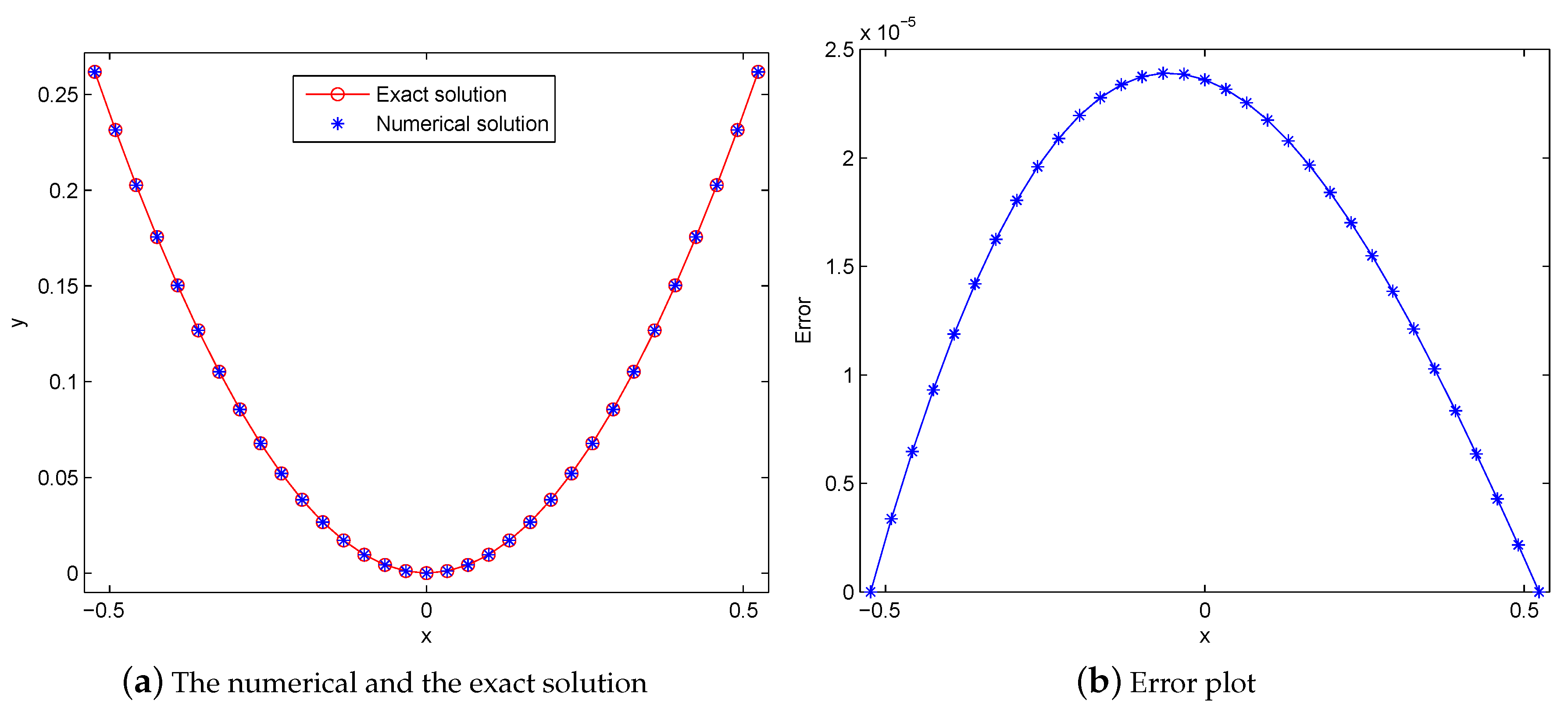
In Figure 1a, we show the exact solution and the numerical results obtained by the proposed method. The corresponding error curve are also shown in Figure 1b. These results coincide with the results listed in Table 2.

Example 4.

Consider the linear differential equation with variable coefficients [3,5]:

$$y^{″}+xy=(3-x-x^2+x^3)sinx+4xcosx,0\le x\le 1.$$

(23)

with boundary conditions $y^{\prime }\left(0\right)=-1,y^{\prime }\left(1\right)=2sin1.$

The analytic solution of (23) is $y=(x^2-1)sinx$. In

Table 3. Maximum errors and elapsed CPU times in Example 4.

n	Ramadan et al. [3]		Srivastava et al. [5]		Our Method
	${\mathit{e}}^{\mathit{\infty }}$	Time (s)	${\mathit{e}}^{\mathit{\infty }}$	Time (s)	${\mathit{e}}^{\mathit{\infty }}$	Time (s)
4	$4.946\times {10}^{-2}$	$1.78\times {10}^{-4}$	$5.927\times {10}^{-3}$	$5.33\times {10}^{-3}$	$2.710\times {10}^{-3}$	$2.48\times {10}^{-4}$
8	$1.231\times {10}^{-2}$	$1.89\times {10}^{-4}$	$6.173\times {10}^{-4}$	$5.34\times {10}^{-3}$	$6.700\times {10}^{-4}$	$2.62\times {10}^{-4}$
16	$3.081\times {10}^{-3}$	$2.61\times {10}^{-4}$	$1.797\times {10}^{-4}$	$5.54\times {10}^{-3}$	$1.670\times {10}^{-4}$	$3.68\times {10}^{-4}$
32	$7.704\times {10}^{-4}$	$3.43\times {10}^{-4}$	$3.495\times {10}^{-5}$	$5.72\times {10}^{-3}$	$4.183\times {10}^{-5}$	$5.94\times {10}^{-4}$
64	$1.926\times {10}^{-4}$	$5.75\times {10}^{-4}$	$6.702\times {10}^{-6}$	$6.28\times {10}^{-3}$	$1.046\times {10}^{-5}$	$1.10\times {10}^{-3}$
128	$4.800\times {10}^{-5}$	$1.62\times {10}^{-3}$	$1.179\times {10}^{-6}$	$7.36\times {10}^{-3}$	$2.615\times {10}^{-6}$	$2.25\times {10}^{-3}$

, we list the maximum errors and the elapsed CPU time. The numerical results obtained by implementing the methods [3,5] are also listed for comparison. Note that the elapsed CPU time for the same routine in Matlab may be different every time. In order to count the time accurately, we took the average of all runtimes of 100 independent runs as the elapsed CPU time.

On one hand, our method is more accurate than Ramadan’s method [3] and comparable to Srivastava’s method [5]. On the other hand, the runtime of our method is less than that of Srivastava’s method and comparable to Ramadan’s method. This indicates that Srivastava’s method can achieve the best precision in our experiment, while our method is superior in the term of elapsed CPU time. This is because we only need to solve a tridiagonal linear system instead of solving a penta-diagonal system in [5], which is much easier to implement.

Clearly, the proposed method is efficient, therefore it provides a new approach to deal with second order linear differential equations.

6. Conclusions

Based on the analytic solutions to the linear differential equation with constant coefficients, we propose an numerical method for second order differential equations in this paper. The analytic solutions are used to construct the approximation function and the local truncation error is analyzed. Numerical examples have shown the effectiveness of the proposed method. Compared with the other methods, we only need to solve a tridiagonal system, which is much easier to implement.

References

- Griffiths, D.F.; Higham, D.J. Numerical Methods for Ordinary Differential Equations; Springer: London, UK, 2010. [Google Scholar]
- Usmani, R.A. The use of quartic splines in the numerical solution of a fourth-order boundary value problem. J. Comput. Appl. Math. 1992, 44, 187–200. [Google Scholar] [CrossRef] [Green Version]
- Ramadan, M.A.; Lashien, I.F.; Zahra, W.K. Polynomial and nonpolynomial spline approaches to the numerical solution of second order boundary value problems. Appl. Math. Comput. 2007, 184, 476–484. [Google Scholar] [CrossRef]
- Ramadan, M.A.; Lashien, I.F.; Zahra, W.K. High order accuracy nonpolynomial spline solutions for 2μth order two point boundary value problems. Appl. Math. Comput. 2008, 204, 920–927. [Google Scholar] [CrossRef]
- Srivastava, P.K.; Kumar, M.; Mohapatra, R.N. Quintic nonpolynomial spline method for the solution of a second order boundary-value problem with engineering applications. Comput. Math. Appl. 2011, 62, 1707–1714. [Google Scholar] [CrossRef] [Green Version]
- Noor, M.A.; Tirmizi, I.A.; Khan, M.A. Quadratic non-polynomial spline approach to the solution of a system of second order boundary-value problems. Appl. Math. Comput. 2007, 179, 153–160. [Google Scholar]
- Zahra, W.K.; Mhlawy, A.M.E. Numerical solution of two-parameter singularly perturbed boundary value problems via exponential spline. J. King Saud Univ. Sci. 2013, 25, 201–208. [Google Scholar] [CrossRef] [Green Version]
- Lodhi, R.K.; Mishra, H.K. Quintic B-spline method for solving second order linear and nonlinear singularly perturbed two-point boundary value problems. J. Comput. Appl. Math. 2017, 319, 170–187. [Google Scholar] [CrossRef]
- Zahra, W.K. A smooth approximation based on exponential spline solutions for nonlinear fourth order two point boundary value problems. Appl. Math. Comput. 2011, 217, 8447–8457. [Google Scholar] [CrossRef]
- Al-Said, E.A.; Noor, M.A. Quartic spline method for solving fourth order obstacle boundary value problems. J. Comput. Appl. Math. 2002, 143, 107–116. [Google Scholar] [CrossRef] [Green Version]
- Ideon, E.; Oja, P. Linear/linear rational spline collocation for linear boundary value problems. J. Comput. Appl. Math. 2014, 263, 32–44. [Google Scholar] [CrossRef]
- Rashidinia, J.; Ghasemi, M. B-spline collocation for solution of two-point boundary value problems. J. Comput. Appl. Math. 2011, 235, 2325–2342. [Google Scholar] [CrossRef] [Green Version]
- Wanner, G. Solving Ordinary Differential Equations II; Springer: Berlin/Heidelberg, Germany, 1991. [Google Scholar]
- Ahmad, G.I.; Shelly, A.; Kukreja, V.K. Cubic Hermite Collocation Method for Solving Boundary Value Problems with Dirichlet, Neumann, and Robin Conditions. Int. J. Eng. Math. 2014, 2014, 365209. [Google Scholar]
- Ge, Y.; Cao, F. Multigrid method based on the transformation-free HOC scheme on nonuniform grids for 2D convection diffusion problems. J. Comput. Phys. 2011, 230, 4051–4070. [Google Scholar] [CrossRef]
Figure 1.
Numerical results in Example 2 ().