Machine Learning-Based Prediction of the Seismic Bearing Capacity of a Shallow Strip Footing over a Void in Heterogeneous Soils

Abstract

The seismic bearing capacity of a shallow strip footing above a void displays a complex dependence on several characteristics, linked to geometric problems and to the soil properties. Hence, setting analytical models to estimate such bearing capacity is extremely challenging. In this work, machine learning (ML) techniques have been employed to predict the seismic bearing capacity of a shallow strip footing located over a single unsupported rectangular void in heterogeneous soil. A dataset consisting of 38,000 finite element limit analysis simulations has been created, and the mean value between the upper and lower bounds of the bearing capacity has been computed at the varying undrained shear strength and internal friction angle of the soil, horizontal earthquake accelerations, and position, shape, and size of the void. Three machine learning techniques have been adopted to learn the link between the aforementioned parameters and the bearing capacity: multilayer perceptron neural networks; a group method of data handling; and a combined adaptive-network-based fuzzy inference system and particle swarm optimization. The performances of these ML techniques have been compared with each other, in terms of the following statistical performance indices: coefficient of determination (${\mathrm{R}}^2$); root mean square error ($\mathrm{RMSE}$); mean absolute percentage error; scatter index; and standard bias. Results have shown that all the ML techniques perform well, though the multilayer perceptron has a slightly superior accuracy featuring noteworthy results (${\mathrm{R}}^2=$ 0.9955 and $\mathrm{RMSE}=$ 0.0158).

1. Introduction

Underground voids may be caused by human actions or by the dissolution of soluble substances. Mining, digging aqueducts, the creation of sewerage networks and municipal facilities, and tunneling operations are examples of those human activities, whereas chemical interactions of calcareous and dolomite soils, and soluble rock dissolution, fall into the class of natural causes [1,2]. The voids, especially in urban areas, may be located adjacent to, or below shallow footings. In such cases, the performance of strip footings can be significantly affected by the presence of the underground voids, which therefore require special attention in the design process. A number of factors are linked to the impact of voids on the bearing capacity of strip footings, and they all have to be accounted for concurrently to achieve an optimal design, even in such adverse situations. In the engineering practice, void existence may adversely affect the stability of constructions, leading to a differential settlement of superstructures or the collapse of foundations.

To date, various studies have been conducted to investigate the bearing capacity of strip footings above voids, by using either theoretical or experimental methods. Preliminary studies examined the fundamental issues of the problem, see examples [3,4,5,6,7,8]. In those works, the focus was on the bearing capacity of strip footings over a single void. Later, Kiyosumi et al. [9] carried out a set of centrifuge tests over multiple voids, and the results were assessed through the PLAXIS finite element code. Kiyosumi, Kusakabe, and Ohuchi [10] then analyzed the bearing capacity of a strip footing on stiff grounds with voids, and they classified the failure patterns for a single hole into three categories: roof failure; sidewall failure; and combined failure. Yamamoto et al. [11], in a case characterized by multiple voids, demonstrated that closely spaced tunnels showed a good correlation between the results of finite element simulations and upper-bound limit analysis.

This problem was investigated using small strain kinematics. Lee, Jeong, and Ko [12] quantified the influence of single and dual continuous voids, allowing for a wide variety of geometries and material combinations on the undrained vertical load bearing capacity of strip footings. Lee, Jeong, and Ko [13] also studied the effect of load inclination. Lee, Jeong, and Lee [14] examined the undrained bearing capacity factors of ring footings, to assess the impact of the friction angle in heterogeneous soils. The results showed that, by increasing the inside-to-outside-radius ratio, the value of the soil bearing capacity factor is reduced, whereas when the ratio is reduced, the size of the plastic zones gets enhanced—the bearing capacity also rises with the soil heterogeneity. Lavasan et al. [15] offered a new framework for estimating the bearing capacity of a strip footing over voids, and showed that the bearing capacity is significantly affected by the void’s geometry and position. Chakraborty and Sawant [16] focused on the impact of pseudo-static horizontal earthquake forces on the bearing capacity of strip footings placed over an unsupported circular tunnel in undrained clay.

More recently, the finite element limit analysis (FELA) method was used by Xiao et al. [17]. Design charts were given for a reduction factor to estimate the ultimate bearing capacity of a strip footing over a rock mass with voids. Xiao, Zhao, and Zhao [18] applied the same method to assess the undrained bearing capacity above voids in two-layered clays. Zhou et al. [19] instead used the discontinuity layout optimization approach to determine the bearing capacity above square voids in cohesive-frictional soils, reporting typical failure patterns. Lee and Kim [20] investigated the bearing capacity above multiple square voids in sandy soils and purely cohesive clays, and they also explored the effect of load inclination. Wu et al. [21] studied the effects of the depth and geometry of the voids, and of the eccentricity of loading on the bearing capacity. Recently, Zhang et al. [22] investigated the impact of seismic loading on the bearing capacity of undrained clay with voids.

In order to deal with complex problems, which are usually difficult to attack with a purely model-based approach, machine learning (ML) is currently experiencing a burst of popularity in applications, and also in the civil engineering field, see examples [23,24,25,26,27,28,29,30,31,32]. Regarding the foundation engineering field, neural networks have been employed to estimate the settlement and the load carrying capacity of pile foundations [33,34,35], and of isolated shallow footings [36,37,38,39,40].

To the best of the authors’ knowledge, no research has been carried out so far to predict the bearing capacity of a shallow strip footing above a void by means of approaches based on ML tools. In the present study, a first attempt is made to set an extensive database dealing with the various factors affecting the said bearing capacity for strip footings above a single unsupported void in either heterogeneous or homogenous soils, under seismic and quasi-static excitations. The considered factors are:

• Soil cohesion
• Soil internal friction angle
• Heterogeneity
• Distance of the void from the central line of the footing
• Depth of the void
• Shape and size of the void
• Horizontal earthquake acceleration.

Results have been obtained as lower and upper bounds on the load bearing capacity of the strip footing via the FELA method. First, a sensitivity analysis has been conducted to quantify the effects of these parameters on the ultimate footing bearing capacity. Next, to predict the seismic bearing capacity, the multiplayer perceptron (MLP), group method of data handling (GMDH), and adaptive-network-based fuzzy inference system and particle swarm optimization (ANFIS-PSO) techniques have been adopted.

The proposed procedure, based on the ML tools, can therefore be framed in the following way: for all the problems characterized by the geometry of strip footing and a void similar to the one here considered, and by heterogeneous solids, of which the main properties affecting their resistance are cohesion and friction angle within the investigated ranges, the said ML tools can be assumed already tuned and trained. Practitioners can then use the ML-based models as a kind of black-box, to automatically and quickly obtain an estimation of the seismic bearing capacity of any shallow strip footing, so that the detrimental effects induced by the interaction with the buried, unsupported void can be easily quantified.

The remainder of this paper is organized as follows: in Section 2, the attacked problem is defined in detail, and the modeling in Optum G2 is validated with literature results to ensure the accuracy of the solutions in the database. The results of a parametric study, performed to assess how the aforementioned factors affect the solution, are reported in Section 3. The ML tools adopted to learn the link between the input factors and the footing bearing capacity, namely the output, are described in Section 4. The outcomes generated by the ML algorithms are given in Section 5 in statistical terms to assess the accuracy in reproducing all the ground-truth results in the dataset, and in Section 6 for a case study featuring a specific geometry, in order to provide a concrete idea concerning the accuracy of the attained results. The conclusions of the present work and foreseen future developments are then expressed in Section 7. Finally, Appendix A gathers the equations relevant to the MLP and GMDH models, and the MATLAB code for the adopted ANFIS-PSO model.

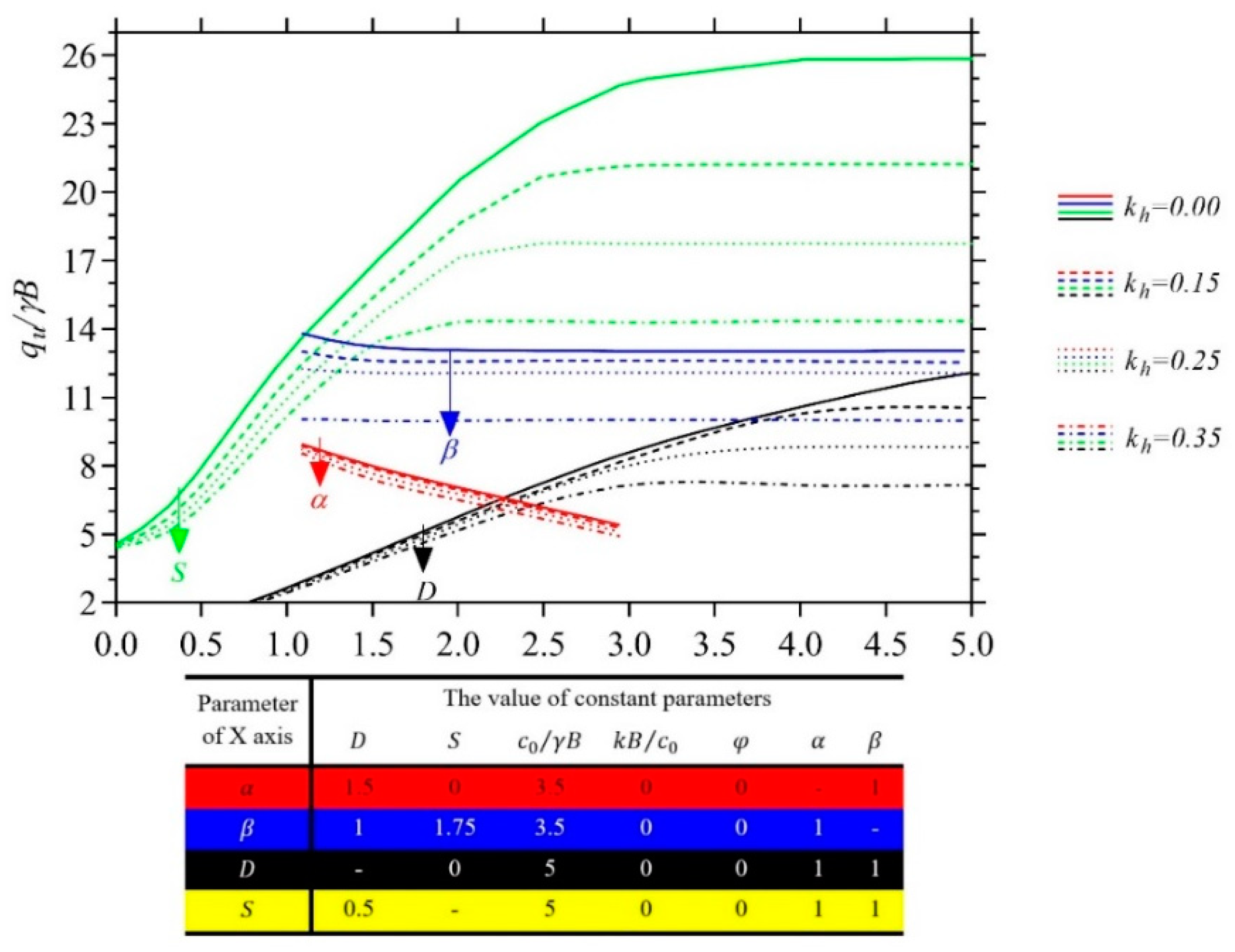
2. Problem Definition

A literature review, regarding the topic of concern here, has pointed out that the interaction between a strip footing and voids displays interesting complexities. Several parameters affect the interaction of the foundation, the soil, and the voids/tunnels. These parameters are listed in

Table 1. Parameters investigated in recent research.

Parameter	Yamamoto et al. [11]	J.K. Lee, Jeong and Ko [12]	Lavasan [15]	Xiao, Zhao and Zhao [18]	Zhou et al. [19]
Internal friction angle	√				√
Cohesion	√	√		√	√
Depth of void	√	√	√	√	√
Eccentricity of void	√	√	√	√	√
Shape of void		√	√	√
Size of void		√	√	√

, along with the papers where they were already accounted for.

In Figure 1, the two-dimensional geometry of the specific problem considered in this work is depicted. Assuming the strip footing and the tunnel to extend infinitely in the out-of-plane direction, plane strain conditions are adopted in the analysis. The strip footing is assumed rigid, featuring a rough surface in contact with the heterogeneous soil. According to the proposed setting, the following dimensionless variables are adopted to parametrize the problem:

-

Horizontal seismic acceleration coefficient $k_h,$ which is equal to the ratio between the horizontal earthquake-induced ground acceleration and the gravity acceleration.

-

Ratio $\alpha =W/B$ between the void width $W$ and the foundation width $B$.

-

Ratio $\beta =H/B$ between the void height $H$ and the foundation width $B$.

-

Undrained shear strength $c_0/\gamma B$ of the soil at the ground level, $c_0$ being the cohesion of the soil, and $\gamma$ the soil specific gravity.

-

Rate of change $kB/c_0$ of the cohesion $c$ with the depth, according to the law:

$$c=c_0+kz$$

(1)

where $c_0$ is, as stated above, the value of the cohesion at the free surface $z=0$. For a homogeneous soil, $k$ is null, whereas for heterogeneous soils, $k$ is positive—additional details can be found in [41,42].

-

Internal friction angle $\phi$ of the soil in the drained state.

-

Depth $D=Z/B$ of the void, $Z$ being the burial depth of the upper side (roof) of the void.

-

Eccentricity $S=X/B$ of the void, $X$ being the horizontal distance of the center of the void from the centerline of the foundation.

Accounting for all the parameters listed above, the (dimensionless) undrained seismic ultimate bearing capacity $Q$ of a strip footing placed above the void is assumed to be:

$$Q=\frac{q_u}{\gamma B}=f\left(\frac{c_0}{\gamma B},\frac{kB}{c_0},\phi ,S, D, \alpha , \beta ,k_h\right)$$

(2)

To set the database for digging with the ML algorithms, FELA analyses have been carried out to determine $Q$ using the Optum G2 software [43]. By exploiting mesh adaptivity, the code allows for the mesh to be progressively refined, namely reducing the characteristic size of the elements where plastic dissipation takes place. On its own, this mesh adaption allows for the bounds to be tightened on the ultimate bearing capacity $Q$ generated by each analysis, as described below, without any (potentially not objective) user intervention.

This approach is broadly used in geotechnical engineering to solve stability problems [11,44] and ascertain the footing bearing capacity [18,45,46,47,48]. Through the FELA method, which is a mixture of the finite element and the classical limit analysis of plasticity, lower and upper bounds on the ultimate bearing capacity of the foundation can be obtained. For further details regarding the theoretical background and the numerical implementation of this method, readers are referred to [49,50,51] for the lower bound finite element limit theory, and to [49,51,52,53] for the upper bound one. Notably, a striking advantage of the FELA approach is that preliminary assumptions related to the failure surface are not needed [54].

Meshes consisting of triangular elements have been adopted, independently of the values of the geometrical parameters introduced above. To start the iterative mesh adaption procedure, each model has been assumed to be made of 1000 elements. Through h-adaptivity, elements have been automatically generated or reduced in size where shear stress concentration and dissipation is going to affect the solution, until a limit of 10,000 elements has been attained. Such initial and final numbers of elements have been chosen on the basis of the results presented in [55,56], the latter to specifically keep the computational burden of each analysis below a critical threshold.

The Mohr–Coulomb failure criterion has been used to model the soil behavior, while the strip footing has been modeled as a weightless rigid plate. The ultimate load bearing capacity has then been defined through a multiplier for a uniform load applied to the footing, and automatically increased until the formation of collapse mechanisms.

In the analyses, a strip footing with a width $B=1$ m has been placed on soil with a specific weight of 20$\mathrm{kN}/{\mathrm{m}}^3$. To avoid any perturbation to the solution induced by the domain boundaries, a model with a width of $40B$ and a depth of $20B$ has been considered. The contact of the soil with the bedrock has been modelled by constraining both the horizontal and the vertical displacements along the bottom surface. Along the side boundaries, only the horizontal components of the displacements have instead been restrained.

The pseudo-static method has been adopted to assess the seismic performance of the foundation over the cavity. For this purpose, the value of the horizontal acceleration coefficient $k_h$ has been exploited, and once the upper and lower bounds on $q_u$ or $Q$ at collapse have been computed, the relevant mean value has been assumed as the representative result for each model. An example of the adopted models is depicted in Figure 2, where the typical FELA adaptive mesh of the Optum G2 software, along with the adopted boundary conditions, are sketched.

To validate the modeling approach, the results of some studies in the literature have been considered for comparison purposes. First, as seen in [57], the bearing capacity of the foundation has been computed via the lower bound FELA method, in case of horizontal seismic loadings. The relevant results are compared in Figure 3, in terms of the bearing capacity factor $N_{\gamma },$ to show how they perfectly match the available ones. Second, a comparison with the studies of [57,58,59,60,61,62,63,64] has been made through the data gathered in

Table 2. Bearing capacity of the foundation: comparison with literature data in terms of the capacity factor $N_{\mathsf{\gamma }}$.

$\mathit{\phi }$ (°)	${\mathit{N}}_{\mathit{\gamma }}$
	Present Study		Yang et al.	Booker	Hansen	Chen	Michalowski	Kumar	Hjiaj et al.	Zhao and Yang
	LB	UB
20	1.41	3.11	2.98	3.01	2.95	5.200	4.47	3.43	2.89	2.92
25	3.55	7.07	6.75	6.95	6.76	11.40	9.77	7.18	6.59	-
30	10.9	16.2	15.29	16.06	15.07	25.00	21.39	15.57	14.90	14.96
35	25.4	37.8	35.73	37.13	33.92	57.00	48.68	35.16	34.80	-
40	63.8	96.1	88.54	85.81	79.54	114.0	118.83	85.73	85.86	86.76

. Such a comparison is provided in terms of the bearing capacity factor, at a varying value of the internal friction angle $\phi$. The results again show a good agreement with those published, and correctly bound almost all of them. Third, in

Table 3. Bearing capacity of the foundation: comparison with literature data, in terms of the capacity factor $N_c$ for a strip footing above a single void.

$\mathit{D} \mathit{\alpha }$	${\mathit{N}}_{\mathit{c}}$
	Present Study ${\mathit{c}}_{\mathit{u}}=60\mathbf{kPa}$	Present Study ${\mathit{c}}_{\mathit{u}}=300\mathbf{kPa}$	$(\mathbf{Lee} \mathbf{et} \mathbf{al}.) {\mathit{c}}_{\mathit{u}}=60\mathbf{kPa}$	(Kiyosumi et al.) ${\mathit{c}}_{\mathit{u}}=60\mathbf{kPa}$	(Kiyosumi et al.) ${\mathit{c}}_{\mathit{u}}=300\mathbf{kPa}$	(Zhou et al.) ${\mathit{c}}_{\mathit{u}}=60\mathbf{kPa}$	$(\mathbf{Zhou} \mathbf{et} \mathbf{al}.) {\mathit{c}}_{\mathit{u}}=300\mathbf{kPa}$
1.50	1.71	1.98	2.02	1.68	1.95	1.68	1.92
2.00	2.55	2.95	3.11	2.50	2.90	2.50	2.92
2.50	3.39	3.98	3.90	3.34	3.88	3.34	3.88
3.00	4.14	4.80	4.62	4.17	4.85	4.18	4.83
3.50	4.66	5.08	5.10	5.00	5.82	5.00	5.19
4.00	5.11	5.15	5.16	5.84		5.18	5.21
4.50	5.13	5.15	5.16			5.21	5.21
5.00	5.13	5.15	5.16			5.21	5.21

, a further comparison is provided for the bearing capacity factor $N_c,$ allowing for the presence of a void at different depths $D$ beneath the strip footing central line, see [10,12,19]. It has been assumed that the opening width is equal to the surface footing width, and is located within an utterly cohesive soil at an undrained state with cohesion varying in the range $60-300$ kPa. Results are shown again to agree well with the reference ones.

3. Parametric Study

Before moving to the setting of the database for the application of the ML algorithms, a parametric analysis is here presented. To evaluate the effect of the parameters listed in Section 2 on the seismic behavior of the system, a set of analyses has been designed. In an undrained situation, for a strip footing with a rough surface on the ground level, the pseudo-static acceleration coefficient at the threshold of strip footing sliding is $0.38$. To study the effect of earthquakes, values of $k_h$= 0, 0.15, 0.25, and 0.35 have been accounted for.

In the following, the outcomes of the parametric analysis are subdivided, in order to focus first on the effects of parameters related to the soil behavior, and next on the effects of parameters related to the geometry and position of the void.

3.1. Soil Parameters

The results in Figure 4 provide insights into the variation of the dimensionless bearing capacity $Q=\frac{q_u}{\gamma B},$ see Equation (2), induced by the soil features, under different values of the horizontal seismic acceleration coefficient $k_h$. Figure 4a shows the outcome of the analysis for a broad range of values of the undrained shear strength. The graph confirms that for a low shear strength, that is for $c_0/\gamma B<1,$ the model can be unstable (especially regarding the lower bound state): void collapse occurs without any loading and the value of $Q$ gets close to zero, though it cannot be computed due to the instability of the model. As far as the effect of $kB/c_0$ on the seismic and static bearing capacity of the shallow footing is concerned, Figure 4a also shows that the bearing capacity raises slightly under seismic conditions, however, it then becomes independent of $kB/c_0$.

Results in Figure 4b instead show that by increasing the angle of internal friction of the soil, the bearing capacity of the strip footing increases as well: for $\phi \le$ 30°, the bearing capacity increases at a low rate, but for larger values, it keeps increasing sharply.

3.2. Void Parameters

Results are depicted in Figure 5 showing the variation of the bearing capacity induced by varying the void parameters related to its shape and location. At constant seismic action measured through $k_h,$ the capacity $Q=q_u/\gamma B$ is shown to increase with the void depth $D$ until a saturation value that depends on its own $k_h$. Similar conclusions can be drawn considering the effect of the horizontal distance S from the footing central line. It has also been reported that the bearing capacity decreases as the ratio $\alpha$ related to the void width increases, with instability triggered for a value approaching $\alpha =3$. For a void located below the centerline of the footing (namely $S=0$), the effect of the ratio $\beta$ related to the void height is to first marginally reduce the bearing capacity, and then attain a constant value.

As the data have to be handled through ML approaches, the quality of the dataset is one of the dominant aspects to assure the accuracy of the predictions. To assess the bearing capacity of the strip footing above a void, the adopted dataset has been made of 38,000 models, each one featuring its own values of the parameters describing the soil properties and the void geometry. According to the parametric study presented above, the values of the parameters have been selected within their domains to cover all the effective situations related to the interaction between the strip and the void. The aforementioned effective values of the parameters are collected in

Table 4. Effective parameters and selected values for each model.

Shape of Void		Effective Parameters								Total Number of Scenarios
		${\mathit{c}}_0/\mathit{\gamma }\mathit{B}$	$\mathit{k}\mathit{B}/{\mathit{c}}_0$	$\mathit{D}$	$\mathit{S}$	$\mathbf{S}\mathbf{h}\mathbf{a}\mathbf{p}\mathbf{e}$		$\mathit{\phi }$	${\mathit{k}}_{\mathit{h}}$
						$\mathit{\alpha }$	$\mathit{\beta }$
Rectangular	Selected Values	2, 4, 6, 8	0, 0.5, 1	0.75, 1.5, 3, 4.5, 6	0, 1, 2, 3.5, 5	1	3	0, 10, 20, 30, 40	0, 0.1, 0.2, 0.3
						1	2
						1	1
						2	1
						3	1
	Number of scenarios	4	3	5	5	5		5	4	30,000
Square	Selected Values	2, 4, 6, 8	0	0.75, 1.5, 3, 4.5, 6	0, 1, 2, 3.5, 5	0.5	0.5	0, 10, 20, 30, 40	0, 0.1, 0.2, 0.3
						1.5	1.5
						2.0	2.0
						2.5	2.5
	Number of scenarios	4	1	5	5	4		5	4	8000
Total number of models considered										38,000

.

As already remarked, for each analysis, only the average value between the upper and lower bounds on the strip footing bearing capacity has been considered as an entry of the dataset.

4. Machine Learning Techniques

To learn and then estimate the seismic bearing capacity of the shallow strip footing above the void, three nonlinear machine learning algorithms have been adopted: an MLP artificial neural network (ANN); the GMDH; and a combined ANFIS–PSO.

According to Table 4, the database for digging is characterized by eight input parameters ($c_0/\gamma B,$ $kB/c_0,D,$ $S,$ $\alpha ,$ $\beta ,$ $\phi ,$ and $k_h$) and only one output ($Q=q_u/\gamma B$). In the following, a detailed description of these methods is provided, along with the impact of the relevant hyperparameters of their performance. Hyperparameters are defined here as the algorithm-dependent parameters that control the learning process.

4.1. Multilayer Perceptron (MLP)

McCulloch and Pitts first introduced ANNs as a powerful predictive tool in [66]. ANNs are a programming paradigm which try to mimic the brain’s structure. They are broadly employed in artificial intelligence problems, from simple pattern-recognition tasks to advanced symbolic manipulation. ANN-based models process the available data during a training stage, assessing the network output to efficiently and accurately match some available targets in case of a supervised approach, like the one here adopted based on the FELA results included in the dataset. ANNs can be used for modeling complex systems in virtually any science [67,68].

MLP is a class of ANNs, and stands as an evolution of the perceptron neural network originally developed in the 1960s, see [69]. For a general problem, MLP is able to provide a nonlinear map $f:{ℝ}^k\to {ℝ}^h,$ in case of an input layer made of $k$ neurons (input values) and an output layer made of $h$ neurons (output values). It also consists of an arbitrary number of hidden layers, with a variable number of neurons. The neurons are storage cells for scalar values, obtained by an activation function applied to the neuron values in the previous layer.

For our problem, a preliminary analysis has been performed to identify the optimal architecture of the MLP, in terms of the number of neurons in the hidden layers, to accurately describe the correlation between input and output of the analyzed dataset. In this regard, one-hidden-layer and two-hidden-layer ANNs have been investigated—to speed-up the optimization procedure, only 5% of the data has been adopted at this stage. To this aim, in [70], it was suggested that the ratio between the number of data and the number of input and output variables should be greater than five, to attain an appropriate performance of MLP—in the present case, the mentioned ratio results are $1900/9=211,$ which are much larger than the minimum value suggested.

Figure 6 provides a comparison of the behaviors of all the considered architectures at the end of training. Results are reported in terms of the root mean square error ($\mathrm{RMSE}$), given by:

$$\mathrm{RMSE}=\sqrt{\frac{1}{n}{\displaystyle \sum }_{i=1}^n{\left(Q_{OG2 i}-Q_{Model i}\right)}^2}$$

(3)

which has been assumed as the loss function to be minimized during the training. In Equation (3): $n$ is the total number of data; and for the $i$-th model, $Q_{OG2 i}$ is the load bearing capacity obtained with the Optum G2 software, whereas $Q_{Model i}$ is the value estimated through the MLP algorithm.

To assess the effects of the hyperparameters on the ANN accuracy, the plot in Figure 6 shows the final value of $\mathrm{RMSE}$ as a function of the total number of neurons in the MLP. The continuous line represents the solution obtained with the one-hidden-layer ANN, which is obviously uniquely defined by the number of neurons in the layer itself. The dashed lines represent the solutions for the two-hidden-layer ANNs, and for each of them, the label in the chart represents the number of neurons in its first hidden layer. Each point in this graph has been computed as the average value out of ten repetitions of the training process, to also assure robustness against stochastic effects. What can be seen from this analysis is that the ANN featuring one hidden layer only, almost surely provides the best performance. Furthermore, for a number of neurons larger than 20, there is no noticeable improvement in the final value of the $\mathrm{RMSE}$. Accordingly, and in order to minimize the computational costs, the 8-20-1 ANN architecture has been adopted henceforth.

The effect of the proportioning of the data handled for training, validation, and testing of the MLP has been investigated next. As before, 5% of the data have been handled to evaluate the performance of MLP for different values of proportioning, and the results are shown in Figure 7 at varying values of the percentage of training data. The best performance has been obtained for 65% of the dataset employed for training, 30% for validation, and the remaining 5% for testing. Therefore, the numbers of samples used for the various stages of the MLP-based analysis are as follows: out of the total 38,000 data, 24,700 were used for training, 11,400 for testing, and 1900 for validation.

4.2. Group Method of Data Handling (GMDH)

The GMDH algorithm, which was first proposed in [71], combines mathematical modeling approaches and black-box nonlinear system identification, aiming to learn the complex relationship between input and output in the provided dataset. By means of a polynomial transfer function (Volterra functional series), GMDH allows the neurons to become more complex units.

Unlike MLP, this method can be considered a particular type of self-organized ANN, which employs natural selection to control the size, complexity, and accuracy of the network. The main fields of application of GMDH are the modeling of complex systems, function approximation, nonlinear regression, and pattern recognition (more information can be found in example [72]).

Even for this architecture, a preliminary analysis has been performed to identify the optimal values of the number of layers and of the maximum number of neurons in a layer, to enhance its effectiveness. Like for the MLP, for this stage of the analysis, 5% of the available data have been used. The effects of the aforementioned hyperparameters on the RMSE at the end of training are depicted in Figure 8. The graph shows that, when the number of layers is larger than six, the RMSE is only marginally affected. Moreover, it can be seen that an optimal value for the maximum number of neurons in a layer is 12. For values larger than this threshold, only a small variation of the RMSE is reported, which is arrived at by largely increasing the cost of training.

To run the GMDH algorithm, a parameter called “selection pressure”, which can be thought of as a threshold to determine the number of neurons in each layer, must be set. Its value ranges from zero to define the no-pressure mode (to select all the generated neurons), to one to define the maximum pressure mode (to select no neurons from all the generated ones). Hence, the lower the value of the selection pressure, the more complex the structure of the GMDH and the higher the related computational effort. A trade-off has thus been arranged, in such a way that its value does not negatively affect the performance of the algorithm while being maximized. According to the results collected in Figure 9, an optimal value of this hyperparameter has been set to 0.2.

As for the MLP, the effect of data proportioning for training and testing has been investigated. Figure 10 shows that, independently of the number of layers, the percentage of training data does not significantly affect the GMDH performance. Therefore, 50% of the entire dataset has thus been selected for it.

4.3. Combined Adaptive-Network-Based Fuzzy Inference System and Particle Swarm Optimization (ANFIS-PSO)

ANFIS is known to be a useful ML approach to solve function approximation problems [73]. ANFIS, which uses ANN standard training algorithms, is structured with if-else rules and input-output fuzzy joined data [74]. To simulate complex nonlinear mapping, a trained ANN and fuzzy logic work together in different imprecise and unpredictable noisy spaces [75]. Further aspects about ANFIS are reported in [27].

The PSO is based on competition and collaboration among particles [76,77]. It performs a local search and leads to fast convergence in minimizing the objective function, see [78,79]. The most striking advantage of this optimization algorithm over others is that the use of swarming particles makes the process robust against the solution getting entrapped into local minima of the handled objective function, since each particle renews its position and pathway based on its and others’ information.

In this work, PSO has been used to provide the membership functions of ANFIS, assumed to be Gaussian ones, thereby decreasing the computation costs for a given topology of ANFIS itself. A thorough explanation on the combined ANFIS-PSO algorithm can be found in [80].

In order to enhance the performance of this algorithm, the critical hyperparameters that need to be set are the number of iterations, or in other words, the stopping criterion, and the number of particles in the population handled at each iteration. Although exact rules for the swarm size selection are not reported in the literature, the main issue linked to it is that, when the problem dimension increases, the swarm size does increase as well, and may quickly become unmanageable [81].

By setting the maximum number of iterations to 5000 and the number of particles varying in a range between five and 95, Figure 11 shows the evolution of RMSE. It can be seen that a number of iterations equal to 5000 looks appropriate to converge to the final solution, independently of the number of particles. As depicted in the inset of Figure 11, after 5000 iterations, the solution linked to 65 particles has shown the best performance.

The initial and final values $W_1$ and $W_2$ of the inertia weight also need to be set. This weight provides a trade-off between the concentration of particles in their neighborhoods, and the exploration of new points in the parameter space. Higher values of the weight allow more new points to be explored, while lower values allow the concentration capability of PSO to be boosted. The value of this hyperparameter has been linearly reduced during the run, so that the search effort is essentially focused on the exploration at the initial steps (governed by $W_1$), while it is focused more on exploitation at the latter phases (governed by $W_2$) of the run.

Figure 12 shows the sensitivity of the PSO performance to $W_1$ and $W_2$. In the graph, different colors are related to different values of $W_1,$ whereas different line formats are associated to different values of $W_2$. It clearly emerges that the red lines associated to $W_1=0.8$ provide the best performance. Furthermore, the continuous lines linked to $W_2=0.2$ give rise to the minimum final value of RMSE and, in all the cases, to the steepest descents in its evolution.

Other hyperparameters to tune in the analysis are the cognitive and social acceleration coefficients $C_1$ and $C_2,$ which describe the weighting of the stochastic acceleration terms that move particles towards the best objective so far ($C_1$), and to the best objective of swarm particles ($C_2$). By increasing the cognitive acceleration coefficient value, the attraction of particles towards the best objective is enhanced, while their appeal towards the best goal of swarm particles is reduced. Since the social acceleration coefficient does the exact opposite, the relation between the values of the two coefficients is critical and may affect the behavior of the algorithm. Concerning the ratios $C_1/C_2$ and $C_2/C_1,$ we have considered eight different values in the investigation, plus the threshold characterized by $C_1=C_2$. According to the results shown in Figure 13, which provides the evolution of $\mathrm{RMSE}$ during the optimization by PSO as a function of the cognitive and social acceleration coefficients $C_1$ and $C_2,$ the best performance has been obtained for $C_1=1$ and $C_2=1.5$.

As was done for the other algorithms, the effect of the proportioning of data has been investigated. Figure 14, which shows the evolution of $\mathrm{RMSE}$ during the optimization by PSO, testifies that the optimal percentage of training data is 70%. Accordingly, out of the 38,000 data, 26,600 have been used for training and 11,400 for testing.

5. Results and Discussion

In this section, the performances of the three selected ML tools are compared. As metrics for the said performances, the following statistical indices have been adopted to measure the discrepancy between ground-truth and the predicted values of the seismic load bearing capacity:

$${\mathrm{R}}^2={\left[{\displaystyle \sum }_{i=1}^n\left(Q_{OG2 i}-\overline{Q_{OG2}}\right)\left(Q_{Model i}-\overline{Q_{Model}}\right)/\sqrt{{\displaystyle \sum }_{i=1}^n{\left(Q_{OG2 i}-\overline{Q_{OG2}}\right)}^2{\displaystyle \sum }_{i=1}^n{\left(Q_{Model i}-\overline{Q_{Model}}\right)}^2}\right]}^2$$

(4)

$$\mathrm{MAPE}=\frac{1}{n}{\displaystyle \sum }_{i=1}^n\left|Q_{OG2 i}-Q_{Model i}\right|/Q_{OG2 i}$$

(5)

$$\mathrm{SI}=\mathrm{RMSE}/\overline{Q_{OG2}}$$

(6)

$$\mathrm{BIAS}=\frac{1}{n}{\displaystyle \sum }_{i=1}^n\left(Q_{OG2 i}-Q_{Model i}\right)$$

(7)

${\mathrm{R}}^2,$ $\mathrm{MAPE},$ $\mathrm{SI},$ and $\mathrm{BIAS}$ being, respectively, the coefficient of determination, the mean absolute percentage error, the scatter index, and the standard bias. Besides these indices, the $\mathrm{RMSE}$ introduced in Equation (3) has been adopted too. In these equations $i=1,\dots ,n$ is an index running over the instances in the dataset. It is also worth recalling that $Q_{OG2 i}$ is the numerical value of the dimensionless load bearing capacity $Q=q_u/\gamma B$ generated by the Optum G2 software, while $Q_{Model i}$ is the corresponding value provided by the trained ML tool (the overbar stands for the average value of the corresponding variable).

Table 5. Performance of the ML algorithms, in term of the adopted statistical indices.

Algorithm	${\mathbf{R}}^2$	$\mathbf{R}\mathbf{M}\mathbf{S}\mathbf{E}$	$\mathbf{M}\mathbf{A}\mathbf{P}\mathbf{E}$	$\mathbf{S}\mathbf{I}$	$\mathbf{B}\mathbf{I}\mathbf{A}\mathbf{S}$
MLP	0.9955	0.0158	−0.0101	−0.0189	−0.0001
GMDH	0.8417	0.0938	−0.0750	−0.1123	−0.0009
ANFIS-PSO	0.9542	0.0505	−0.0017	−0.0605	0.8997

gathers the values of all the statistical indices introduced above to assess the performance of each ML approach. It can be seen that MLP is more accurate than GMDH and ANFIS-PSO in catching the structural response, as shown by the ${\mathrm{R}}^2,$ $\mathrm{RMSE},$ $\mathrm{SI},$ and $\mathrm{BIAS}$ values. The same trend is also shown in the parity plots given in Figure 15, where the estimations of the seismic bearing capacity $Q=q_u/\gamma B$ of the shallow strip footing are compared with the ground-truth values. Output provided by MLP is shown to be much less scattered than the others, and the linear interpolation of all the pairs of results is well aligned with the (perfect fit) bisector of the quadrant. In spite of the relatively small value of the $\mathrm{BIAS},$ due to the fact that each single term in the sum is purposely taken with its own sign, the GMDH model performs worse, as reported by the large scatter and also by the deviation from the perfect fit line of the linear interpolant.

The goodness of the fit of the results has been also studied: Figure 16 provides a comparison between the FELA and the foreseen seismic bearing capacity of the shallow strip footing. For this comparison, only 1% of the instances in the dataset have been randomly selected, so as to provide a clear view of the quality of data fitting. It results that the seismic bearing capacity computed by the ML techniques matches relatively well with their FELA counterparts, and the minor scattering around them is obviously in accordance with the results reported in Figure 15.

6. A Case Study

In this section, the results obtained in this study in terms of trained ANN-based models, are adopted for a practical engineering problem to assess the seismic bearing capacity of a strip footing placed over an unsupported void. It has been assumed that the strip footing, featuring $B=$ 8 m, is located over homogeneous soil characterized by $c_0=$ 300 kPa, $\gamma =$ 18 kN/m³, and $\phi =$ 20°. As shown in Figure 17, the footing is placed near a square void, which is 4 m wide and 4 m high, and the center of which is placed at a depth of 12 m and at a distance of 16 m from the footing centerline. To predict the undrained seismic bearing capacity in the specific case $k_h=$ 0.2, the ML method introduced in this research can be adopted as follows:

First, the nondimensional input parameters of the problem need to be computed to obtain:

$$\frac{c_0}{\gamma B}=\frac{300 \left[\mathrm{kPa}\right]}{18 [\mathrm{kN}/{\mathrm{m}}^3]·8 \left[\mathrm{m}\right]}=2.08$$

$$\frac{kB}{c_0}=0$$

$$\alpha =\frac{W}{B}=\frac{4 \left[\mathrm{m}\right]}{8 \left[\mathrm{m}\right]}=0.5$$

$$\beta =\frac{H}{B}=\frac{4 \left[\mathrm{m}\right]}{8 \left[\mathrm{m}\right]}=0.5$$

According to Figure 17, where the center of the void is shown to be placed at a depth of 12 m and at a distance of 16 m from the footing centerline, the additional nondimensional depth and eccentricity parameters amount to:

$$D=\frac{Z}{B}=\frac{12-4/2 \left[\mathrm{m}\right]}{8 \left[\mathrm{m}\right]}=1.25$$

$$S=\frac{X}{B}=\frac{16 \left[\mathrm{m}\right]}{8 \left[\mathrm{m}\right]}=2$$

For this case study, the Optum G2 software has provided the lower and upper bounds on the ultimate bearing capacity as 3193.65 kPa and 3301.85 kPa, respectively, so the mean value has been given as 3247.75 kPa. The ML methods here investigated have instead provided the estimations reported in

Table 6. Case study: seismic bearing capacity of the strip footing estimated by the investigated ML tools, and error with respect to the ground-truth to the value given by the Optum G2 software.

Algorithm	$\mathbf{Estimate} {\mathit{q}}_{\mathit{u}}\left[\mathbf{kPa}\right]$	Error
MLP	3184.23	1.96%
GMDH	3325.11	2.38%
ANFIS-PSO	3091.24	4.82%

, along with the relevant errors with respect to the aforementioned ground-truth value. As already pointed out in Section 5, MLP is shown to perform better than the two alternative tools, giving rise to a representative error smaller than 2%. Very similar results can be obtained for any other geometry falling within the interval of characteristic parameters allowed for while assembling the dataset of Table 4.

7. Conclusions

In this study, the seismic bearing capacity of a strip footing placed over an unsupported void has been assessed. Dimensionless factors describing the horizontal seismic acceleration, the soil strength and heterogeneity, the internal friction angle of the soil, the shape, size, depth, and eccentricity of the void have been accounted for.

Three ML techniques have been exploited to estimate the aforementioned bearing capacity: MLP; GMDH; and ANFIS-PSO. All the hyperparameters affecting the performance of the ML models have been investigated, to ensure the attainment of optimal solutions in all the cases. The results obtained by training the ML models have shown a good fitting of the seismic bearing capacity provided by numerical FELA simulations, here handled as the ground-truth data. More specifically, MLP, and ANFIS-PSO have performed better than GMDH. Overall, almost independently of the adopted statistical performance index used to assess the goodness of the fit of the models, MLP has been shown to be superior to the other models. This outcome has also been testified by means of concrete results regarding a case study.

A major concern regarding the use of a data-driven ML approach to foresee the information related to limit states of a structural system, typically highly sensitive to some parameters unknown or difficult to assess, is related to the quality of the dataset. In future activities, the proposed approach will be fed also with experimental data, to assess the credibility of the ML models. To this purpose, collecting empirical data of the seismic bearing capacity of the strip footing above voids would be worthwhile, to finally establish an effective tool to design strip footing, especially in urban areas.

In this study, only rectangular voids have been considered. Having established the reliability of the offered methodology, additional datasets will be considered in the future to allow for voids with a different geometry, aiming to increase the awareness of strip footing behavior over voids.

References

1. Fam, M.A.; Cascante, G.; Dusseault, M.B. Large and small strain properties of sands subjected to local void increase. J. Geotech. Geoenviron. Eng. 2002, 128, 1018–1025. [Google Scholar] [CrossRef]
2. Tharp, T.M. Mechanics of upward propagation of cover-collapse sinkholes. Eng. Geol. 1999, 52, 23–33. [Google Scholar] [CrossRef]
3. Al-Tabbaa, A.; Russell, L.; O’Reilly, M. Model tests of footings above shallow cavities. Ground Eng. 1989, 22, 39–41. [Google Scholar]
4. Badie, A.; Wang, M.C. Stability of spread footing above void in clay. J. Geotech. Eng. 1984, 110, 1591–1605. [Google Scholar] [CrossRef]
5. Baus, R.L.; Wang, M.C. Bearing capacity of strip footing above void. J. Geotech. Eng. 1983, 109, 1–4. [Google Scholar] [CrossRef]
6. Wang, M.C.; Badie, A. Effect of underground void on foundation stability. J. Geotech. Eng. 1985, 111, 1008–1019. [Google Scholar] [CrossRef]
7. Wang, M.C.; Hsieh, C.W. Collapse load of strip footing above circular void. J. Geotech. Eng. 1987, 113, 511–515. [Google Scholar] [CrossRef]
8. Es-haghi, M.S.; Abbaspour, M.; Rabczuk, T. Factors and Failure Patterns Analysis for Undrained Seismic Bearing Capacity of Strip Footing Above Void. Int. J. Geomech. 2021, 21, 04021188. [Google Scholar] [CrossRef]
9. Kiyosumi, M.; Kusakabe, O.; Ohuchi, M.; Le Peng, F. Yielding pressure of spread footing above multiple voids. J. Geotech. Geoenviron. Eng. 2007, 133, 1522–1531. [Google Scholar] [CrossRef] [Green Version]
10. Kiyosumi, M.; Kusakabe, O.; Ohuchi, M. Model tests and analyses of bearing capacity of strip footing on stiff ground with voids. J. Geotech. Geoenviron. Eng. 2011, 137, 363–375. [Google Scholar] [CrossRef]
11. Yamamoto, K.; Lyamin, A.V.; Wilson, D.W.; Sloan, S.W.; Abbo, A.J. Stability of dual circular tunnels in cohesive-frictional soil subjected to surcharge loading. Comput. Geotech. 2013, 50, 41–54. [Google Scholar] [CrossRef]
12. Lee, J.K.; Jeong, S.; Ko, J. Undrained stability of surface strip footings above voids. Comput. Geotech. 2014, 62, 128–135. [Google Scholar] [CrossRef]
13. Lee, J.K.; Jeong, S.; Ko, J. Effect of load inclination on the undrained bearing capacity of surface spread footings above voids. Comput. Geotech. 2015, 66, 245–252. [Google Scholar] [CrossRef]
14. Lee, J.K.; Jeong, S.; Lee, S. Undrained bearing capacity factors for ring footings in heterogeneous soil. Comput. Geotech. 2016, 75, 103–111. [Google Scholar] [CrossRef]
15. Lavasan, A.A.; Talsaz, A.; Ghazavi, M.; Schanz, T. Behavior of shallow strip footing on twin voids. Geotech. Geol. Eng. 2016, 34, 1791–1805. [Google Scholar] [CrossRef]
16. Chakraborty, D.; Sawant, A.S. Seismic bearing capacity of strip footing above an unsupported circular tunnel in undrained clay. Int. J. Geotech. Eng. 2017, 11, 97–105. [Google Scholar] [CrossRef]
17. Xiao, Y.; Zhao, M.; Zhao, H.; Zhang, R. Finite element limit analysis of the bearing capacity of strip footing on a rock mass with voids. Int. J. Geomech. 2018, 18, 04018108. [Google Scholar] [CrossRef]
18. Xiao, Y.; Zhao, M.; Zhao, H. Undrained stability of strip footing above voids in two-layered clays by finite element limit analysis. Comput. Geotech. 2018, 97, 124–133. [Google Scholar] [CrossRef]
19. Zhou, H.; Zheng, G.; He, X.; Xu, X.; Zhang, T.; Yang, X. Bearing capacity of strip footings on c–φ soils with square voids. Acta Geotech. 2018, 13, 747–755. [Google Scholar] [CrossRef]
20. Lee, J.K.; Kim, J. Stability charts for sustainable infrastructure: Collapse loads of footings on sandy soil with voids. Sustainability 2019, 11, 3966. [Google Scholar] [CrossRef] [Green Version]
21. Wu, G.; Zhao, M.; Zhao, H.; Xiao, Y. Effect of eccentric load on the undrained bearing capacity of strip footings above voids. Int. J. Geomech. 2020, 20, 04020078. [Google Scholar] [CrossRef]
22. Zhang, R.; Feng, M.; Xiao, Y.; Liang, G. Seismic Bearing Capacity for Strip Footings on Undrained Clay with Voids. J. Earthq. Eng. 2020, 1–4. [Google Scholar] [CrossRef]
23. Das, S.K.; Samui, P.; Sabat, A.K. Application of artificial intelligence to maximum dry density and unconfined compressive strength of cement stabilized soil. Geotech. Geol. Eng. 2011, 29, 329–342. [Google Scholar] [CrossRef]
24. Erzin, Y.; Gumaste, S.D.; Gupta, A.K.; Singh, D.N. Artificial neural network (ANN) models for determining hydraulic conductivity of compacted fine-grained soils. Can. Geotech. J. 2009, 46, 955–968. [Google Scholar] [CrossRef]
25. Es-Haghi, M.S.; Shishegaran, A.; Rabczuk, T. Evaluation of a novel Asymmetric Genetic Algorithm to optimize the structural design of 3D regular and irregular steel frames. Front. Struct. Civ. Eng. 2020, 14, 1110–1130. [Google Scholar] [CrossRef]
26. Mishra, A.K.; Kumar, B.; Dutta, J. Prediction of Hydraulic Conductivity of Soil Bentonite Mixture Using Hybrid-ANN Approach. J. Environ. Inform. 2016, 27, 98–105. [Google Scholar] [CrossRef]
27. Safari, M.J.; Ebtehaj, I.; Bonakdari, H.; Es-haghi, M.S. Sediment transport modeling in rigid boundary open channels using generalize structure of group method of data handling. J. Hydrol. 2019, 577, 123951. [Google Scholar] [CrossRef]
28. Shishegaran, A.; Varaee, H.; Rabczuk, T.; Shishegaran, G. High correlated variables creator machine: Prediction of the compressive strength of concrete. Comput. Struct. 2021, 247, 106479. [Google Scholar] [CrossRef]
29. Martinez, R.F.; Lorza, R.L.; Delgado, A.A.; Pullaguari, N.O. Optimizing presetting attributes by softcomputing techniques to improve tapered roller bearings working conditions. Adv. Eng. Softw. 2018, 123, 13–24. [Google Scholar] [CrossRef]
30. Lostado Lorza, R.; Escribano García, R.; Fernandez Martinez, R.; Martínez Calvo, M.Á. Using genetic algorithms with multi-objective optimization to adjust finite element models of welded joints. Metals 2018, 8, 230. [Google Scholar] [CrossRef] [Green Version]
31. Lostado-Lorza, R.; Escribano-Garcia, R.; Fernandez-Martinez, R.; Illera-Cueva, M.; Mac Donald, B.J. Using the finite element method and data mining techniques as an alternative method to determine the maximum load capacity in tapered roller bearings. J. Appl. Log. 2017, 24, 4–14. [Google Scholar] [CrossRef]
32. Lostado Lorza, R.; Corral Bobadilla, M.; Martínez Calvo, M.Á.; Villanueva Roldan, P.M. Residual stresses with time-independent cyclic plasticity in finite element analysis of welded joints. Metals 2017, 7, 136. [Google Scholar] [CrossRef] [Green Version]
33. Das, S.K.; Basudhar, P.K. Undrained lateral load capacity of piles in clay using artificial neural network. Comput. Geotech. 2006, 33, 454–459. [Google Scholar] [CrossRef]
34. Lee, I.M.; Lee, J.H. Prediction of pile bearing capacity using artificial neural networks. Comput. Geotech. 1996, 18, 189–200. [Google Scholar] [CrossRef]
35. Momeni, E.; Nazir, R.; Armaghani, D.J.; Maizir, H. Prediction of pile bearing capacity using a hybrid genetic algorithm-based ANN. Measurement 2014, 57, 122–131. [Google Scholar] [CrossRef]
36. Acharyya, R.; Dey, A. Assessment of failure mechanism of a strip footing on horizontal ground considering flow rules. Innov. Infrastruct. Solut. 2018, 3, 49. [Google Scholar] [CrossRef]
37. Behera, R.N.; Patra, C.R.; Sivakugan, N.; Das, B.M. Prediction of ultimate bearing capacity of eccentrically inclined loaded strip footing by ANN: Part II. Int. J. Geotech. Eng. 2013, 7, 165–172. [Google Scholar] [CrossRef]
38. Giasi, C.I.; Cherubini, C.; Paccapelo, F. Evaluation of compression index of remoulded clays by means of Atterberg limits. Bull. Eng. Geol. Environ. 2003, 62, 333–340. [Google Scholar] [CrossRef]
39. Kuo, Y.L.; Jaksa, M.B.; Lyamin, A.V.; Kaggwa, W.S. ANN-based model for predicting the bearing capacity of strip footing on multi-layered cohesive soil. Comput. Geotech. 2009, 36, 503–516. [Google Scholar] [CrossRef]
40. Shahin, M.A.; Maier, H.R.; Jaksa, M.B. Predicting settlement of shallow foundations using neural networks. J. Geotech. Geoenviron. Eng. 2002, 128, 785–793. [Google Scholar] [CrossRef]
41. Osman, A.S.; Mair, R.J.; Bolton, M.D. On the kinematics of 2D tunnel collapse in undrained clay. Geotechnique 2006, 56, 585–595. [Google Scholar] [CrossRef] [Green Version]
42. Sloan, S.W.; Assadi, A. Undrained stability of a square tunnel in a soil whose strength increases linearly with depth. Comput. Geotech. 1991, 12, 321–346. [Google Scholar] [CrossRef]
43. Krabbenhoft, K.; Lyamin, A.; Krabbenhoft, J. Optum Computational Engineering (OptumG2). Computer Software. 2015. Available online: https://www.optumce.com (accessed on 12 August 2021).
44. Wilson, D.W.; Abbo, A.J.; Sloan, S.W.; Lyamin, A.V. Undrained stability of dual square tunnels. Acta Geotech. 2015, 10, 665–682. [Google Scholar] [CrossRef]
45. Beygi, M.; Keshavarz, A.; Abbaspour, M.; Vali, R.; Saberian, M.; Li, J. Finite element limit analysis of the seismic bearing capacity of strip footing adjacent to excavation in c-φ soil. Geomech. Geoengin. 2020, 1–4. [Google Scholar] [CrossRef]
46. Beygi, M.; Vali, R.; Keshavarz, A. Pseudo-static bearing capacity of strip footing with vertical skirts resting on cohesionless slopes by finite element limit analysis. Geomech. Geoengin. 2020, 1–4. [Google Scholar] [CrossRef]
47. Shiau, J.S.; Lyamin, A.V.; Sloan, S.W. Bearing capacity of a sand layer on clay by finite element limit analysis. Can. Geotech. J. 2003, 40, 900–915. [Google Scholar] [CrossRef] [Green Version]
48. Vali, R.; Beygi, M.; Saberian, M.; Li, J. Bearing capacity of ring foundation due to various loading positions by finite element limit analysis. Comput. Geotech. 2019, 110, 94–113. [Google Scholar] [CrossRef]
49. Lyamin, A.V.; Sloan, S.W. Lower bound limit analysis using non-linear programming. Int. J. Numer. Methods Eng. 2002, 55, 573–611. [Google Scholar] [CrossRef]
50. Lyamin, A.V. Three-Dimensional Lower Bound Limit Analysis Using Nonlinear Programming. Available online: https://nova.newcastle.edu.au/vital/access/manager/Repository/uon:37296 (accessed on 12 August 2021).
51. Sloan, S.W. Lower bound limit analysis using finite elements and linear programming. Int. J. Numer. Anal. Methods Geomech. 1988, 12, 61–77. [Google Scholar] [CrossRef]
52. Krabbenhoft, K.; Lyamin, A.V.; Sloan, S.W.; Wriggers, P. An interior-point algorithm for elastoplasticity. Int. J. Numer. Methods Eng. 2007, 69, 592–626. [Google Scholar] [CrossRef]
53. Yu, H.S.; Sloan, S.W.; Kleeman, P.W. A quadratic element for upper bound limit analysis. Eng. Comput. 1994, 11, 195–212. [Google Scholar] [CrossRef] [Green Version]
54. Vali, R.; Saberian, M.; Beygi, M.; Porhoseini, R.; Abbaspour, M. Numerical Analysis of Laterally Loaded Single-Pile Behavior Affected by Urban Metro Tunnel. Indian Geotech. J. 2020, 50, 410–425. [Google Scholar] [CrossRef]
55. Keshavarz, A.; Beygi, M.; Vali, R. Undrained seismic bearing capacity of strip footing placed on homogeneous and heterogeneous soil slopes by finite element limit analysis. Comput. Geotech. 2019, 113, 103094. [Google Scholar] [CrossRef]
56. Íñiguez-Macedo, S.; Lostado-Lorza, R.; Escribano-García, R.; Martínez-Calvo, M.Á. Finite element model updating combined with multi-response optimization for hyper-elastic materials characterization. Materials 2019, 12, 1019. [Google Scholar] [CrossRef] [PubMed] [Green Version]
57. Kumar, J. N γ for rough strip footing using the method of characteristics. Can. Geotech. J. 2003, 40, 669–674. [Google Scholar] [CrossRef]
58. Booker, J.R. Application of Theories of Plasticity to Cohesive Frictional Soils. Available online: https://ses.library.usyd.edu.au/handle/2123/10044 (accessed on 12 August 2021).
59. Chen, W.-F. Limit Analysis and Soil Plasticity; Elsevier Science: Amsterdam, The Netherlands, 1975. [Google Scholar]
60. Hansen, J.B. A Revised and Extended Formula for Bearing Capacity. Dan. Geotech. Inst. Cph. Bull. 1970, 28, 5–11. [Google Scholar]
61. Hjiaj, M.; Lyamin, A.V.; Sloan, S.W. Numerical limit analysis solutions for the bearing capacity factor Nγ. Int. J. Solids Struct. 2005, 42, 1681–1704. [Google Scholar] [CrossRef]
62. Yang, F.; Zheng, X.C.; Zhao, L.H.; Tan, Y.G. Ultimate bearing capacity of a strip footing placed on sand with a rigid basement. Comput. Geotech. 2016, 77, 115–159. [Google Scholar] [CrossRef]
63. Yun, G.; Bransby, M.F. The undrained vertical bearing capacity of skirted foundations. Soils Found. 2007, 47, 493–505. [Google Scholar] [CrossRef] [Green Version]
64. Zhao, L.H.; Yang, F. Construction of improved rigid blocks failure mechanism for ultimate bearing capacity calculation based on slip-line field theory. J. Cent. South Univ. 2013, 20, 1047–1057. [Google Scholar] [CrossRef]
65. Kumar, J.; Chakraborty, D. Seismic bearing capacity of foundations on cohesionless slopes. J. Geotech. Geoenviron. Eng. 2013, 139, 1986–1993. [Google Scholar] [CrossRef]
66. McCulloch, W.S.; Pitts, W. A logical calculus of the ideas immanent in nervous activity. Bull. Math. Biophys. 1943, 5, 115–133. [Google Scholar] [CrossRef]
67. Pal, S.K.; Mitra, S. Multilayer perceptron, fuzzy sets, classifiaction. IEEE Trans. Neural Netw. 1992, 3, 683–697. [Google Scholar] [CrossRef] [PubMed]
68. Ruck, D.W.; Rogers, S.K.; Kabrisky, M. Feature selection using a multilayer perceptron. J. Neural Netw. Comput. 1990, 2, 40–48. [Google Scholar]
69. Noriega, L. Multilayer Perceptron Tutorial; School of Computing, Staffordshire University: Shropshire, UK, 2005. [Google Scholar]
70. Gandomi, A.H.; Yang, X.S.; Talatahari, S.; Alavi, A.H. (Eds.) Metaheuristic Applications in Structures and Infrastructures; Newnes: Newton, MA, USA, 2013. [Google Scholar]
71. Ivakhnenko, A.G. The group method of data handling in prediction problems. Sov. Autom. Control 1976, 9, 21–30. [Google Scholar]
72. Farlow, S.J. The GMDH algorithm of Ivakhnenko. Am. Stat. 1981, 35, 210–215. [Google Scholar]
73. Jang, J.S. ANFIS: Adaptive-network-based fuzzy inference system. IEEE Trans. Syst. Man Cybern. 1993, 23, 665–685. [Google Scholar] [CrossRef]
74. Inan, G.Ö.; Göktepe, A.B.; Ramyar, K.A.; Sezer, A.L. Prediction of sulfate expansion of PC mortar using adaptive neuro-fuzzy methodology. Build. Environ. 2007, 42, 1264–1269. [Google Scholar] [CrossRef]
75. Liu, M.; Ling, Y.Y. Using fuzzy neural network approach to estimate contractors’ markup. Build. Environ. 2003, 38, 1303–1308. [Google Scholar] [CrossRef]
76. Eberhart, R.; Kennedy, J. Particle swarm optimization. IEEE Int. Conf. Neural Netw. 1995, 4, 1942–1948. [Google Scholar]
77. El-Zonkoly, A.M. Optimal tuning of power systems stabilizers and AVR gains using particle swarm optimization. Expert Syst. Appl. 2006, 31, 551–557. [Google Scholar] [CrossRef]
78. El-Gallad, A.; El-Hawary, M.; Sallam, A.; Kalas, A. Enhancing the particle swarm optimizer via proper parameters selection. In Proceedings of the IEEE CCECE2002. Canadian Conference on Electrical and Computer Engineering, Winnipeg, MB, Canada, 12–15 May 2002; Volume 2, pp. 792–797. [Google Scholar]
79. Shamshirband, S.; Mosavi, A.; Rabczuk, T. Particle swarm optimization model to predict scour depth around a bridge pier. Front. Struct. Civ. Eng. 2020, 14, 855–866. [Google Scholar] [CrossRef]
80. Basser, H.; Karami, H.; Shamshirband, S.; Akib, S.; Amirmojahedi, M.; Ahmad, R.; Jahangirzadeh, A.; Javidnia, H. Hybrid ANFIS–PSO approach for predicting optimum parameters of a protective spur dike. Appl. Soft Comput. 2015, 30, 642–649. [Google Scholar] [CrossRef]
81. Rezaee Jordehi, A.; Jasni, J. Parameter selection in particle swarm optimisation: A survey. J. Exp. Theor. Artif. Intell. 2013, 25, 527–542. [Google Scholar] [CrossRef]
Figure 1. Problem geometry and notation.
Algorithms 14 00288 g001
Figure 2. Typical FELA mesh for the studied problem with a close-up to show the adaptive mesh refinement around the void, where the collapse mechanism is expected to form.
Algorithms 14 00288 g002
Figure 3. Bearing capacity of the foundation: comparison between the results of the present study and those of [65].
Algorithms 14 00288 g003
Figure 4. Parametric analysis: effects on the bearing capacity Q = q u / γ B under different values of the seismic acceleration coefficient k h , of: (a) the dimensionless soil parameters c 0 / γ B (blue plots) and k B / c 0 (yellow plots); (b) internal friction angle φ .
Algorithms 14 00288 g004
Figure 5. Parametric analysis: effects on the bearing capacity Q = q u / γ B under different values of the seismic acceleration coefficient k h , of the dimensionless void parameters α (red plots), β (blue plots), S (green plots), and D (black plots).
Algorithms 14 00288 g005
Figure 6. MLP: dependence of the RMSE at the end of training on the total number of neurons in the ANN, featuring either one or two hidden layers.
Algorithms 14 00288 g006
Figure 7. Effect of data proportioning on the performance of the one-hidden-layer MLP.
Algorithms 14 00288 g007
Figure 8. GMDH: dependence of the RMSE at the end of training on the maximum number of neurons in a layer and on the maximum number of layers in the ANN.
Algorithms 14 00288 g008
Figure 9. GMDH: dependence of the RMSE at the end of training on the maximum number of layers in the ANN, and on the value of the selection pressure.
Algorithms 14 00288 g009
Figure 10. GMDH: dependence of the RMSE at the end of training on the maximum number of layers in the ANN, and on data proportioning.
Algorithms 14 00288 g010
Figure 11. ANFIS-PSO: evolution of the RMSE during the optimization by PSO, as a function of the number of particles.
Algorithms 14 00288 g011
Figure 12. ANFIS-PSO: evolution of the RMSE during optimization by PSO, as a function of the values W 1 and W 2 of the inertia weight.
Algorithms 14 00288 g012
Figure 13. ANFIS-PSO: evolution of the RMSE during the optimization by PSO, as a function of the values of the cognitive and social acceleration coefficients C 1 and C 2 .
Algorithms 14 00288 g013
Figure 14. ANFIS-PSO: evolution of the RMSE during the optimization by PSO, as a function of data proportioning.
Algorithms 14 00288 g014
Figure 15. Performances of the ML algorithms: parity plots showing the ML output against the corresponding ground-truth numerical values for: (a) all the ML methods and regarding all the data; (b) MLP regarding test and validation data; (c) GMDH regarding test data; (d) ANFIS-PSO regarding test data.
Algorithms 14 00288 g015
Figure 16. Performance of the ML algorithms: comparison between the FELA results and the forecasts provided by the three algorithms for 1% randomly selected data, in terms of the seismic bearing capacity Q = q u / γ B of the shallow strip footing.
Algorithms 14 00288 g016
Figure 17. Geometry of the case study (measures in m).
Algorithms 14 00288 g017