A Novel Approach for Cognitive Clustering of Parkinsonisms through Affinity Propagation

Abstract

Cluster analysis is widely applied in the neuropsychological field for exploring patterns in cognitive profiles, but traditional hierarchical and non-hierarchical approaches could be often poorly effective or even inapplicable on certain type of data. Moreover, these traditional approaches need the initial specification of the number of clusters, based on a priori knowledge not always owned. For this reason, we proposed a novel method for cognitive clustering through the affinity propagation (AP) algorithm. In particular, we applied the AP clustering on the regression residuals of the Mini Mental State Examination scores—a commonly used screening tool for cognitive impairment—of a cohort of 49 Parkinson’s disease, 48 Progressive Supranuclear Palsy and 44 healthy control participants. We found four clusters, where two clusters (68 and 30 participants) showed almost intact cognitive performance, one cluster had a moderate cognitive impairment (34 participants), and the last cluster had a more extensive cognitive deficit (8 participants). The findings showed, for the first time, an intra- and inter-diagnostic heterogeneity in the cognitive profile of Parkinsonisms patients. Our novel method of unsupervised learning could represent a reliable tool for supporting the neuropsychologists in understanding the natural structure of the cognitive performance in the neurodegenerative diseases.

1. Introduction

Cluster analysis is an unsupervised learning technique introduced by Tryon [1], which has an aim to partition objects into homogenous groups for detecting the natural structure as well as the underlying patterns of a dataset according to a measure of similarity, for example geometrical distance. Unlike supervised learning [2,3], clustering is totally data-driven and clustering methods such as traditional hierarchical [4,5] and non-hierarchical [6,7] represent a valuable support to the neuropsychologists [8,9,10] for clustering patients and discovering different patterns of cognitive impairment or multiple cognitive profiles within diagnostic groups [11,12,13,14,15]. Moreover, cluster analysis resulted to be a powerful tool for finding the intra- and inter-diagnostic heterogeneity of psychological and cognitive performance of participants with bipolar disorder or depression syndrome [11,12,13,14] or of patients with Mild Cognitive Impairment [15]. The clustering was also recently applied for exploring patterns of cognitive impairment in Alzheimer’s disease (AD) patients [16], where different cognitive subtypes in the early onset AD subjects were found using the Ward’s method [5] on the regression residuals of the cognitive scores. Together with the wide application of cluster analysis for the cognitive clustering of the AD [17], also the Parkinson’s disease was largely investigated with this technique [18], focusing the attention both on the motor and non-motor symptoms [19,20,21,22,23,24].

However, the vast majority of clustering approaches for understanding the natural structure of cognitive performance in the neurodegenerative diseases [17,18] are traditional methods such as K-means [25], K-median and Ward’s [5], which are less effective, or even inapplicable, on certain kind of cognitive data [8]. Moreover, a crucial issue of these clustering algorithms is the initial choice of the optimum number of clusters for the specific dataset [26,27], which choice, in most applications, could not be based on a priori knowledge [8].

Frey and Dueck [28] proposed in 2007 a clustering algorithm, called affinity propagation (AP), which does not explicitly require to provide the number of clusters, while it identifies an ensemble of representative samples in the dataset to serve as clusters centers. Once these special points, called exemplars, are found, the other data points are connected to the exemplar which has the maximum similarity value [29]. More in detail, the AP algorithm is based on passing messages between data points, where the value of the messages measures the current eligibility of a candidate point to serve as exemplar for another data point [28]. The AP algorithm showed efficiency in handling high dimensional problems [8,28,29,30] and it was applied widely in the physical sciences, especially for the clustering of gene expression.

Given the three main advantages, that is (i) the ability of handling different type of similarity measures, (ii) the automatic discovery of the number of clusters and (iii) the computational efficiency [8], the AP algorithm resulted to be the best candidate approach for exploring, for the first time here, the natural structure of cognitive deficits in Parkinsonisms patients.

In the present work, Parkinson’s disease and Progressive Supranuclear Palsy subjects, together with healthy control participants, were evaluated with the Mini Mental State Examination (MMSE) [23,24,25], which is the most widely used cognitive screening tool. In particular, we wanted to evaluate whether an intra- and inter-diagnostic heterogeneity exists in the altered cognitive functioning of Parkinsonisms and whether the eleven MMSE subscales could capture this possible heterogeneity. With this aim, we proposed a novel approach consisting in clustering through the AP algorithm, the multiple linear regression residuals of the MMSE subscale scores, obtained by controlling the raw data for age, sex and education levels with the method ordinary least squares, for assuring that the discovery of the cognitive clusters is not driven by these three cofounding variables, but only by the diagnosis.

2. Materials and Methods

2.1. Participants

The participants were recruited between 2017 and 2020 by the Movement Disorders Unit of the local University Hospital. The cohort consisted of 140 subjects, divided in 49 Parkinson’s disease patients (PD, mean age ± std 66.7 ± 9.38, 22 females), 48 Progressive Supranuclear Palsy patients (PSP, mean age ± std 70.1 ± 8.32, 22 females), and 44 healthy control subjects (CTRL, mean age ± std 62.6 ± 11.5, 25 females). Clinical diagnosis for PSP patients was established according to the diagnostic criteria for PSP [31,32,33] and clinical diagnosis for PD patients was established according to international diagnostic criteria [34,35]. For each patient, a complete medical history with neurological examination and clinical assessment was performed by trained physicians with more than 10 years of experience in movement disorders. Inclusion criteria for healthy participants were absence of major or unstable medical illness; absence of neurologic (e.g., stroke, movements disorders, epilepsy) and psychiatric disorders; no use of neurological or psychiatric medications; no history of concussion or brain surgery; normal neurological examination. The study was approved by the local Ethical Committee, according to the Helsinki Declaration and written informed consent was obtained from all participants.

2.2. MMSE Assessment

All participants were evaluated with a neuropsychological battery [36] comprising the Mini Mental State Examination (MMSE) [37,38,39] for cognitive functions, always by the same neuropsychologist (M.G.V.) with more than 10 years of experience in neuropsychological assessment of neurological and neurodegenerative diseases. The MMSE is used to screen cognitive impairment and consists of eleven subscales: temporal orientation (TO), orientation in space (OS), registration of three words (Reg), attention and calculation (AC), recall of three words (Rec), language divided into object naming (N) and sentence repetition (SR), praxis (P), writing a sentence (W) chosen by the patient, reading a sentence and performing what is read from the sentence “close your eyes” (CE), and copy a drawing (D). Each subscale has specific instructions and if the participant does not answer a question for any reason, a zero score is awarded. In particular, the score of each MMSE subscale is a discrete value from 0 to a maximum of five points, depending on the subscale. The minimum and maximum values are related to the calculation of the score obtained by the subject at each task of each subscale. In detail, TO subscale contains 5 questions, each task can be assigned a score of 1 if correct or 0 if incorrect (min 0–max 5); OS subscale contains 5 questions, each task can be assigned a score of 1 if correct or 0 if incorrect (min 0–max 5); Reg subscale contains 3 tasks each task can be assigned a score of 1 if correct or 0 if incorrect (min 0–max 3); AC contains 5 calculation operations, each task can be assigned a score of 1 if correct or 0 if incorrect (min 0–max 5); in Rec subscale a score of 1 can be assigned to each word remembered (min 0–max 3); N subscale consists of two tasks each task can be assigned a score of 1 if correct or 0 if incorrect (min 0–max 2); SR contains only one task and each task can be assigned a score of 1 if correct or 0 if wrong (min 0–max 1); P subscale consists of three manual exercise and each task can be assigned a score of 1 if correct or 0 if incorrect (min 0–max 3); W, CE and D subscales consist of one task, each task can be assigned a score of 1 if correct or 0 if incorrect (min 0–max 1) for each subscale.

2.3. Statistical Analysis

The analyses, both statistical and clustering, were performed with a home-made script in python (v. 3.8.6), by using the packages scikit-learn (v. 0.23) [40], numpy (v. 1.19) [41], matplotlib (v. 3.3.3) [42], pandas (v. 1.1.4) [43] and statsmodels (v. 0.12.1) [44]. The implemented code in python can be found in Appendix A.

Differences in the sex distribution among the groups and the clusters were assessed with pairwise Pearson Chi-square tests (p < 0.05). Analysis of variance (ANOVA) was employed for comparing age and education levels in years among the three diagnostic groups (CTRL, PD and PSP) and among the clusters found by our proposed algorithm. An analysis of covariance (ANCOVA) was applied for finding differences in each of the MMSE among the three diagnostic groups and the clusters, by adding age, sex and years of education as covariates.

An analysis of covariance (ANCOVA) was applied with age, sex and education as covariates for comparing the MMSE scores among the groups and among the clusters.

The significance of post-hoc of ANOVA and ANCOVA were corrected for multiple comparisons with Tukey’s honest significant difference (HSD) test (p < 0.05).

2.3.1. Residuals Calculation

We applied a multiple linear regression with the method ordinary least squares (ols) [45] for taking into account the influence of the covariates (age, sex and education years) on the scores of the eleven MMSE subscales. In particular, given Y(n × m), the matrix of the MMSE subscale scores, and X(n × k) the matrix of covariates, the multiple linear regression equation is:

$${\widehat{y}}_{ij}= b_j^0 +b_j^1{x}_{i,1}+\dots + b_j^k{x}_{i,k}+ e_{ij}$$

(1)

where, ${\widehat{y}}_{ij}$ is the predicted value of the i-th observation (i = 1, …, n) of the j-th MMSE subscale (j = 1, …, m) (the dependent variable), $x_i^1$, …, $x_i^k$ are the i-th values of the covariates in X(k) (independent variables), $b_j^0$ is the intercept, $b_j^1$, …, $b_j^k$ are the coefficients and $e_{ij}$ is the model deviation. Then, we obtained the residual $e_{ij}$ of the i-th observation of the j-th MMSE subscale score as:

$$e_{ij}=y_{ij} - {\widehat{y}}_{ij}$$

(2)

that is the difference between the observed and fitted value. The matrix of regression residuals E(n × m) was then used as input for the cluster analysis through affinity propagation, as described in the next section.

2.4. Affinity Propagation

Affinity propagation (AP) is a non-hierarchical clustering method based on graph theory proposed by Frey and Dueck [28], in which each data point is treated as a node of the network, and the nodes exchange iteratively “messages” through the edges of the network itself. An important feature introduced by the AP approach is the concept of exemplars, representative points, which identify centers of clusters. Exemplars are different than centroids of K-Means—barycenter of the points in a cluster—since they have to be one of the actual samples or participants as in the present work. The AP algorithm simultaneously considers all the participants as probable candidates to become centers of the clusters and propagate exchanges of messages between the other participants until the emergence of the best exemplars that maximize the intra-cluster similarity [8,28]. At each iteration of the AP algorithm, the message between two nodes represents the current “affinity” that a sample has for selecting another sample as its exemplar. For this reason, the AP method does not require the initial specification of the number of clusters, as for example in k-centers and k-means approaches.

The AP algorithm requires as input an n × n similarity matrix, S = [s_ij], where n is the number of participants to be clustered and i and j are the participant’s indices. A commonly used measure of distance or dissimilarity is the squared Euclidean distance. If there are two points in an m dimensional space where m is the number of measured variables (the eleven MMSE subscales), then the squared Euclidean distance is defined as:

$$s_{ij}={\displaystyle \sum }_{z=1}^m{\left(e_{iz}-e_{jz}\right)}^2$$

(3)

where e_iz is the value of the z-th variable for the i-th residual and e_ik is the value of the z-th variable for the j-th residual in E(n × m), the matrix of regression residuals, calculated as described in Section 2.3.1. Larger values of s_ij indicate a greater degree of similarity between i and j than smaller values of s_ij. It is assumed that s_ii = 0 (for all 1 ≤ i ≤ n) in the formulation. In the present work, the negative squared Euclidean distance was used, as suggested by Frey and Dueck [28].

The definition of the suitability of each participant for serving as an exemplar is contained in the second input of the AP algorithm: the preferences (p_i, for 1 ≤ i ≤ n, which may also be specified as the n × 1 vector p). In other words, the preferences represent an a priori knowledge of how good a participant could be eligible as an exemplar [29]. Usually, all samples are equally eligible to be an exemplar, thus their value p is the same constant [8,29]. Anyhow, the preferences vector is none other than a control parameter and increasing the value of one sample results in an increase in the likelihood that the sample will be chosen as exemplar [28,29]. The default specification for the preferences is the median of the similarity values (S^M) [8,28], although it has been shown that by using the median, the number of clusters could be dramatically overestimated [8,46]. A reliable alternative is to specify the preference as the minimum of the similarity measures: p_i = S^min, for 1 ≤ i ≤ n, resulting in a smaller number of clusters [28]. For assessing which between the median and the minimum of the similarity matrix is to prefer in the case of the clustering of the MMSE scores, we used both preference values and then we compared their findings with a Silhouette analysis [47] as described in Section 2.5.

In addition to the similarity matrix, the AP algorithm works on two other matrices: the responsibility matrix (R) and the availability matrix (A) [8,28,30]. The final results are stored in a fourth matrix named criterion matrix (C). These three matrices are iteratively updated by the following four equations:

$$r_{ij}\leftarrow s_{ij}- ma{x}_{j^{\prime }s.t. j^{\prime }\ne j}\left\{a_{i{j}^{\prime }}+s_{i{j}^{\prime }}\right\}$$

(4)

$$a_{jj}\leftarrow {{\displaystyle \sum }}_{i^{\prime }s.t. i^{\prime }\ne j}max\left\{0, r_{i^{\prime }j}\right\}$$

(5)

$$a_{ij}\leftarrow min\left\{0, r_{jj}+ {{\displaystyle \sum }}_{i^{\prime }s.t. i^{\prime }\ne i, j}max\left\{0, r_{i^{\prime }j}\right\} \right\}$$

(6)

$$c_{ij}\leftarrow r_{ij}+ a_{ij}$$

(7)

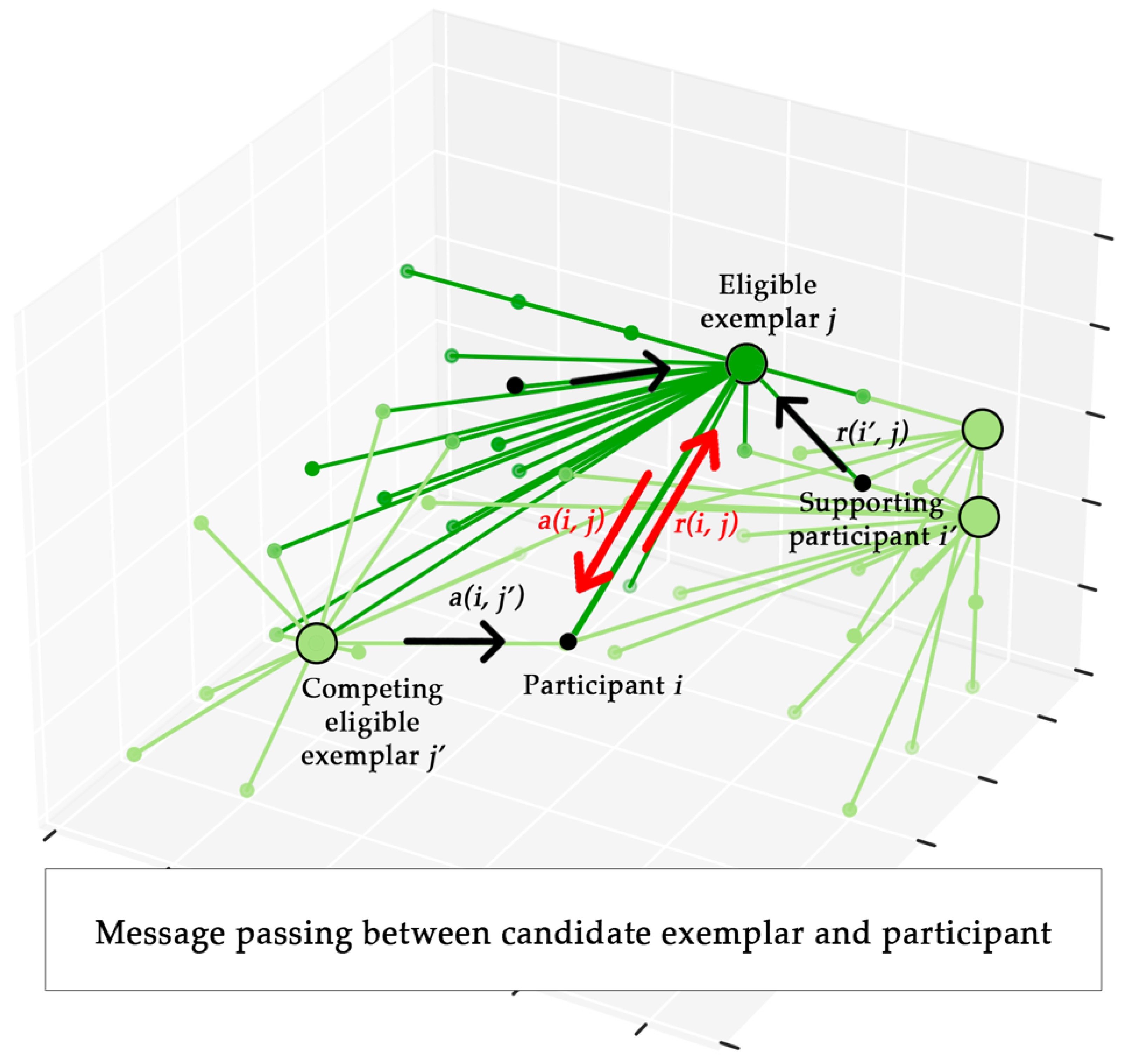
where i and j are respectively the rows and columns indices (1 ≤ i ≤ n and 1 ≤ j ≤ m ) of the associated matrix. Both the responsibility and availability represent the messages exchanged between nodes, bringing two different kind of competition [28]. In particular, the responsibility r(i, j) is sent by the point i to the candidate exemplar point j, and it quantifies the eligibility of the point j to serve as an exemplar for the sample i, considering also other competing exemplar points, e.g., j′ (Figure 1 for a schematic representation). On the contrary, the availability a(i, j) is sent by the candidate exemplar point j to point i, transmitting the information on how is suitable for the point i to choose the point j as its exemplar, considering also the ”opinion” of other supporting point, e.g., i′, regarding the eligibility of j as exemplar (Figure 1 for a schematic representation).

A third input of the AP algorithm is the damping factor d, also called dampening parameter λ [8], which was introduced by Frey and Dueck [28] for assuring the convergence. The purpose of this factor is to add a modest amount of random noise to the similarity matrix and to damp percentage the updates of the responsibility and availability matrices at each iteration t, as follows [30]:

$$r_t=d{r}_{t-1}+ \left(1-d\right)r_t^{’}$$

(8)

$$a_t=d{a}_{t-1}+ \left(1-d\right)a_t^{’}$$

(9)

where r′ and a′ are the undamped updates respectively of the responsibility and availability matrices, calculated by the Equations (4)–(6). The damping factor d is usually a value between 0.5 and 1. Indeed, it has been shown [48] that damping factor values in the interval 0 ≤ d ≤ 0.4 could result in a significant degree of oscillation and issue with convergence of the algorithm [8]. Thus, in the present work, we used the recommended value of 0.5 [8], which means that 50% of the calculation of the responsibility and availability matrices at each iteration is based on information of the previous message exchanged and 50% of the calculation is based on the new message received.

The outputs of the AP algorithm are the number of exemplars ex (clusters) found and the n × 1 cluster assignment vector ξ, containing the labels which are none other than the exemplars (clusters) to which each participant (point) belongs.

The complete algorithm here applied on the MMSE subscale scores, including the calculation of the regression residuals and the application of the AP algorithm for cognitive clustering, is shown in Algorithm 1.

Algorithm 1	Cognitive clustering of regression residuals trough Affinity Propagation
Input:	MMSE subscale scores matrix Y(n × m), covariates matrix X(k), damping factor d
Output:	Number of exemplars ex, cluster assignment vector ξ
1:	initialization: E(n × m), matrix of regression residuals; S(n × n), matrix of similarities; p(n × 1), preference vector of Affinity Propagation;
2:	forj = 1 to m do
3:	fitj = ols(yj ~ x1 + … + xk); fitted model of the j-th column in Y, with x1, …, xk as the columns in X
4:	for i = 1 to n−1 do
5:	eij = yij—fitj.predict(yij); regression residual = the difference between yij and its prediction by fitj
6:	fori = 1 to n do
7:	for j = 1 to m do
8:	for z = 1 to m do
9:	sij = −$\sum _{\mathrm{z}=1}^{\mathrm{m}}{\left(e_{iz}-e_{jz}\right)}^2$; negative squared Euclidean distance between eiz and ejz
10:	pi = Smin OR pi = Smedian
11:	ap = AffinityPropagation(S, p, d);
12:	ex = size(ap.exemplars);
13:	ξ = ap.cluster_membership;

2.5. Clustering Accuracy Assessment

Although previous works [8,28,29,30] showed that the AP algorithm provided satisfactory results, it still could present a limitation due to the arbitrary choice of the initial preferences vector p. For this reason, we compared different clustering results obtained by using the minimum and the median of the similarity matrix. A commonly used approach to assess the quality of clustering results is the Silhouette index, which is a measure of how close each point in a cluster is to the points in its neighboring cluster. Given a cluster X_j (j = 1, …, c where c is the number of clusters found), the Silhouette index Sil_i (i = 1, …, n where n is the number of points in the cluster) of the i-th point in the cluster X_j is given by:

$$Si{l}_i=\frac{mavd\left(i\right)-avd\left(i\right)}{max\left\{avd\left(i\right),mavd\left(i\right)\right\}}$$

(10)

where avd(i) is the mean distance between the i-th point and all the points in the cluster X_j, mavd(i) is the mean minimum distance between the i-th point and all the points in the cluster X_k (k = 1, …, c), and max is the maximum operator. The Silhouette values range varies from −1 to 1, where a value close to 1 could mean that the i-th point was accurately clustered to the optimum exemplar of the cluster. A value near to 0 could suggest that the i-th point could be attributed to the nearest cluster, whereas a value near to −1 could mean that the i-th point was misclassified [47]. Thus, for characterizing the heterogeneity and isolation of a cluster Y_j (j = 1, …, c) it is possible to calculate the cluster Silhouette S_ijl given by:

$$S_{ij}l= {\displaystyle \sum }_{i=1}^m{S}_{i}l\left(i\right)$$

where m is the number of points in S_ijl. The mean value of all the Silhouette indices of all the points in a partition $U\leftrightarrow Y : Y_{l}U\dots Y_{i}U\dots Y_c$, is called Global Silhouette and it is given by the equation:

$$G{S}_u\left(i\right)=\frac{{\sum }_{j=1}^{c}Si{l}_j}{c}$$

(11)

In the present work, we calculated the GS of the clustering obtained by using the median and the minimum of the similarity matrix as preference values, for comparing their quality and assessing the optimal one.

3. Results

3.1. Statistical Analysis

Table 1. Demographic and cognitive data of healthy controls (CTRL), Parkinson’s (PD) and Progressive Supranuclear Palsy (PSP) patients are reported as mean ± standard deviation. The mean and standard deviation of the residuals of the regression with age, sex and education as covariates, are also reported in round brackets.

	CTRL (44)	PD (49)	PSP (48)	p-Value	Post-Hoc
Age	62.6 ± 11.5	66.7 ± 9.38	70.1 ± 8.32	0.002 a	CTRL < PSP b
Female, n	25	22	22	N.S. c
Education	12.5 ± 4.78	9.27 ± 4.74	7.38 ± 5.05	<0.001 a	CTRL > PD b, PSP b
Total MMSE	29.2 ± 1.46	24.8 ± 5.08	20.8 ± 5.27	<0.001 d	CTRL > PD e, PSP e; PD > PSP e
TO	4.93 ± 0.45 (0.241 ± 0.57)	4.49 ± 1.04 (0.100 ± 1.010)	3.85 ± 1.38 (−0.321 ± 1.250)	0.01 d	CTRL > PSP e
OS	4.98 ± 0.15 (0.31 ± 0.567)	4.29 ± 1.15 (−0.025 ± 0.992)	3.81 ± 1.21 (−0.259 ± 0.999)	0.003 d	CTRL > PSP e
Reg	3.00 ± 0 (0.008 ± 0.084)	2.98 ± 0.143 (0.042 ± 0.142)	2.85 ± 0.50 (−0.050 ± 0.485)	N.S.d	N.A.
AC	4.80 ± 0.60 (0.854 ± 0.846)	3.14 ± 1.90 (−0.167 ± 1.590)	2.25 ± 1.77 (−0.616 ± 1.690)	<0.001 d	CTRL > PD e, PSP e
Rec	2.98 ± 0.15 (0.66 ± 0.39)	1.96 ± 1.08 (−0.165 ± 0.970)	1.52 ± 0.9 (−0.441 ± 1.010)	<0.001 d	CTRL > PD e, PSP e
N	1.98 ± 0.15 (−0.02 ± 0.14)	2.00 ± 0 (0.030 ± 0.058)	1.94 ± 0.32 (−0.015 ± 0.303)	N.S. d	N.A.
SR	1.00 ± 0 (0.10 ± 0.04)	0.82 ± 0.39 (−0.055 ± 0.403)	0.81 ± 0.39 (−0.038 ± 0.384)	0.03 d	CTRL > PD e
P	2.93 ± 0.45 (−0.02 ± 0.43)	2.98 ± 0.143 (0.088 ± 0.163)	2.77 ± 0.55 (−0.074 ± 0.540)	N.S.d	N.A.
W	0.91 ± 0.30 (0.16 ± 0.30)	0.67 ± 0.47 (0.065 ± 0.394)	0.29 ± 0.46 (−0.210 ± 0.465)	<0.001 d	CTRL > PSP e; PD > PSP e
CE	0.82 ± 0.40 (−0.003 ± 0.410)	0.84 ± 0.37 (0.123 ± 0.344)	0.52 ± 0.50 (−0.120 ± 0.454)	0.01 d	PD > PSP e
D	0.84 ± 0.37 (0.111 ± 0.270)	0.65 ± 0.48 (0.083 ± 0.394)	0.25 ± 0.44 (−0.185 ± 0.421)	<0.001 d	CTRL > PSP e; PD > PSP e

^a ANOVA p-value, significant at p < 0.05. ^b Post-hoc of ANOVA corrected for multiple comparisons with Tukey’s, significant at p < 0.05. ^c Pairwise Chi-squared, significant at p < 0.05. ^d Analysis of covariance (ANCOVA) with age, sex and education in covariates, significant at p < 0.05. ^e Post-hoc of ANCOVA with age, sex and education in covariates, corrected for multiple comparisons with Tukey’s honest significant difference (HSD) test, significant at p < 0.05. Abbreviations: N.S. = not significant; N.A. = not applicable; CTRL = healthy control; PD = Parkinson’s disease patients; PSP= Progressive Supranuclear Palsy patients.

reported the demographic characteristics and the MMSE total and subscale scores of the three groups of participants, CTRL, PD and PSP patients, together with the results of the statistical analyses, included the pairwise post-hoc findings. The distribution of sex was not significantly different pairwise (p > 0.05). ANOVA revealed significant differences in age only between CTRL and PSP, where the CTRL participants were younger than PSP patients. The education level of the CTRL participants was significantly higher than PD and PSP patients.

The ANCOVA analysis, with age, sex and education level in covariates, showed differences in the MMSE total score, where CTRL participants had higher values than PD and PSP, and PD had higher value than PSP patients.

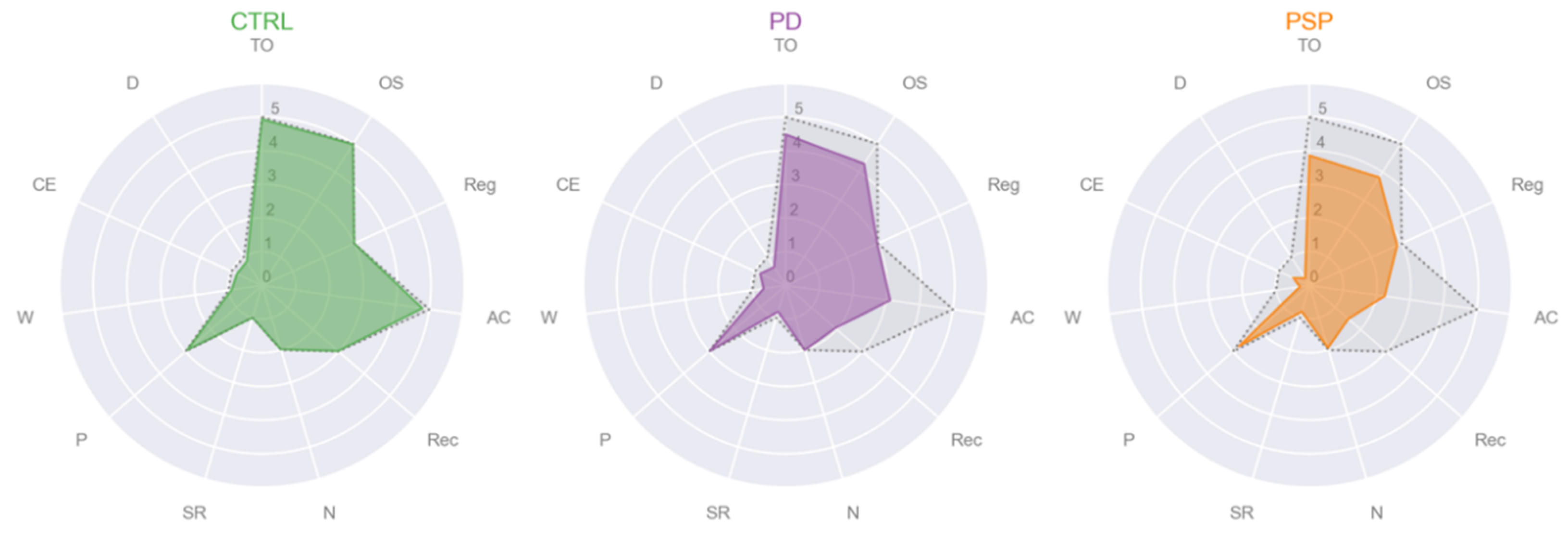
Regarding the MMSE subscales, only registration of three words (Reg), object naming (N) and praxis (P) were not different among groups. Figure 2 depicted the three radar plots of each group, CTRL (in green), PD (in purple) and PSP (in orange), representing the mean values of each MMSE subscale, while in gray and dotted lines the maximum value that each MMSE subscale could reach. PD patients showed cognitive impairment compared to CTRL, in AC, Rec and SR. PSP patients had significant lower scores than the CTRL participants in TO, OS, AC, Rec, W and D. In the comparison between PD and PSP patients, the first had significant higher scores than the second in W, CE and D.

The parameters of the regression models for each MMSE subscale were reported in Appendix B.

3.2. Cluster Analysis

We first applied our proposed algorithm separately on the MMSE scores of the healthy controls group, PD patients and PSP patients for investigating the natural structure of the intra-diagnostic cognitive profiles and then on the whole cohort of CTRL, PD and PSP participants. The comparison of the performance—calculated with the Silhouette index—of each clustering experiment by varying the preference value was reported in

Table 2. Performance—evaluated with the Silhouette index—of the proposed algorithm by varying the preference value of the affinity propagation (AP) clustering.

	Median Preference		Minimum Preference
Group	#Clusters	Silhouette Index	#Clusters	Silhouette Index
CTRL	8	0.302	1	N.A.
PD	7	0.375	2	0.675
PSP	6	0.387	2	0.677
CTRL + PD + PSP	16	0.237	4	0.601

Abbreviation: N.A. = not applicable; CTRL = healthy control; PD = Parkinson’s disease patients; PSP = Progressive Supranuclear Palsy patients.

.

We found an overestimate of the number of clusters (8 clusters) and a poor Silhouette value (0.302) when the proposed algorithm was applied on the control group with the preference value equal to the median of the similarity matrix. In particular, the bigger cluster was comprised of 26 participants, three clusters were comprised of only 1 subject, two clusters were comprised of 3 subjects, one cluster comprised of 4 subjects and the last one was comprised of 5 subjects.

On the contrary, the algorithm with the preference value equal to the minimum of the similarity matrix found only 1 cluster, thus comprising all the healthy control participants. The only exemplar’s demographic values and eleven MMSE scores (as a vector: [TO, OS, Reg, AC, Rec, N, SR, P, W, CE, D]) were:

• Cluster #1 CTRL: male, age 62, education 16, MMSE subscales = [5, 5, 3, 5, 3, 2, 1, 3, 1, 1, 1];

Regarding the PD participants group, we found 7 clusters and a poor value of the Silhouette index (0.375) when the proposed algorithm was applied with the preference value equal to the median of the similarity matrix. In particular, the two biggest clusters were comprised of 13 and 11 PD participants, two clusters were comprised of 7 PD patients, one cluster was comprised of 6 PD patients, one cluster comprised of 3 PD patients and the last one was comprised of 2 PD patients.

A significant improvement of the Silhouette index (0.675) and 2 clusters were found with the preference value equal to the minimum value of the similarity matrix. The exemplars’ demographic values and eleven MMSE subscale scores (as a vector: [TO, OS, Reg, AC, Rec, N, SR, P, W, CE, D]) were:

• Cluster #1 PD: male, age 43, education 13, MMSE subscales = [5, 5, 3, 4, 3, 2, 1, 3, 1, 1, 1];
• Cluster #2 PD: female, age 61, education 8, MMSE subscales = [5, 5, 3, 5, 3, 2, 1, 3, 1, 1, 1];

The first cluster was comprised of 29 PD patients (13 females) with a mean age of 66.4 ± 10.7, a mean education level of 9.14 ± 4.98 and a total MMSE mean score of 22.3 ± 5.09 (TO 4.14±, OS 3.97 ± 1.35, Reg 2.97 ± 0.19, AC 2.07 ± 1.71, Rec 1.62 ± 1.12, N 2 ± 0, SR 0.83 ± 0.38, P 2.97 ± 0.19, W 0.55 ± 0.51, CE 0.72 ± 0.45, D 0.52 ± 0.51). The second cluster was comprised of 20 PD patients (9 females) with a mean age of 67.3 ± 7.09, a mean education level of 9.45 ± 4.50 and a total MMSE mean score of 28.4 ± 1.79 (TO 50±, OS 4.75 ± 0.55, Reg 3 ± 0, AC 4.70 ± 0.73, Rec 2.45 ± 0.83, N 2 ± 0, SR 0.80 ± 0.41, P 3 ± 0, W 0.85 ± 0.37, CE 1 ± 0, D 0.85 ± 0.37). See Figure 3 for the radar plots of the mean values of MMSE subscales of each of the two clusters of PD patients found. The statistical analyses showed that the age, distribution of sex and education level were not significantly different between the two clusters of PD patients (p > 0.05). The ANCOVA, with age, sex and education level in covariates, showed that the total MMSE score, TO, OS, AC, Rec, W, CE and D were significantly different between the two clusters (p < 0.001).

The number of clusters found on PSP patients‘ data was 6 and the Silhouette index was low (0.387) when the preference value was equal to the median of the similarity matrix. In particular, we found 2 bigger clusters with 15 and 11 PSP participants, 2 clusters were comprised of 8 PSP patients, 1 cluster was comprised of 5 PSP patients and 1 cluster comprised of 1 PSP patient.

We found an improvement of the Silhouette index (0.677) and a total of 2 clusters when the preference value was equal to the minimum of the similarity matrix. The exemplars’ demographic values and eleven MMSE subscale scores (as a vector: [TO, OS, Reg, AC, Rec, N, SR, P, W, CE, D]) were:

• Cluster #1 PSP: male, age 57, education 17, MMSE subscales = [5, 5, 3, 2, 1, 2, 1, 3, 0, 1, 0];
• Cluster #2 PSP: male, age 78, education 13, MMSE subscales = [5, 5, 3, 5, 2, 2, 1, 3, 0, 1, 0];

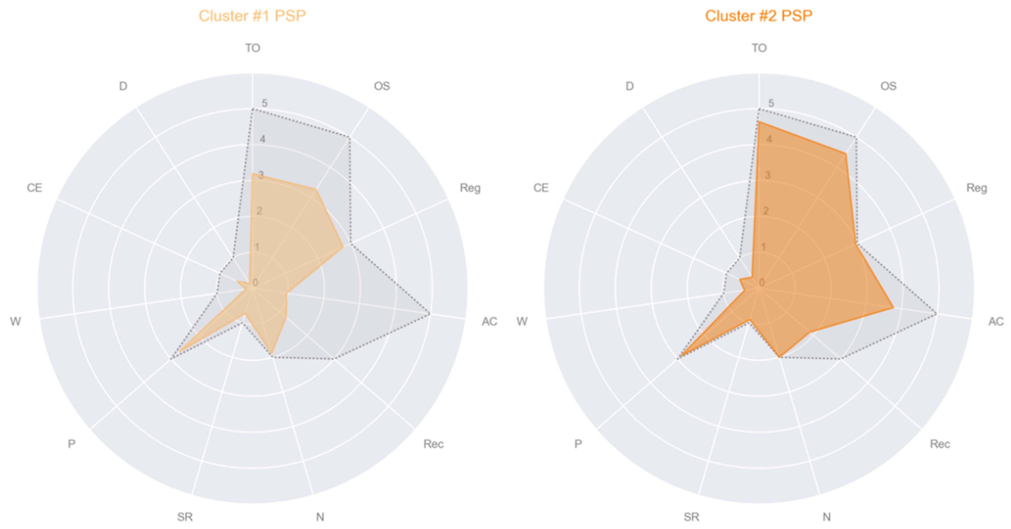
The first cluster was comprised of 26 PSP patients (12 females) with a mean age of 70.3 ± 8.17, a mean education level of 6.88 ± 4.71 and a total MMSE mean score of 17.4 ± 4.31 (TO 3.19 ± 1.52, OS 3.27 ± 1.28, Reg 2.77 ± 0.65, AC 0.96 ± 0.77, Rec 1.23 ± 0.95, N 1.88 ± 0.43, SR 0.73 ± 0.45, P 2.69 ± 0.62, W 0.19 ± 0.40, CE 0.46 ± 0.51, D 0.15 ± 0.37). The second cluster was comprised of 22 PSP patients (10 females) with a mean age of 70.0 ± 8.69, a mean education level of 7.95 ± 5.47 and a total MMSE mean score of 24.9 ± 2.88 (TO 4.64 ± 0.59, OS 4.45 ± 0.74, Reg 2.95 ± 0.21, AC 3.77 ± 1.34, Rec 1.86 ± 071, N 2 ± 0, SR 0.91 ± 0.29, P 2.86 ± 0.47, W 0.41 ± 0.50, CE 0.59 ± 0.50, D 0.36 ± 0.49). See Figure 4 for the radar plots of the mean values of MMSE subscales of each of the two clusters of PSP patients found. The statistical analyses revealed that the age, distribution of sex and education level were not significantly different between the two clusters of PSP patients (p > 0.05). The ANCOVA, with age, sex and education level in covariates, showed that the total MMSE score, TO, OS, AC and Rec were significantly different between the two clusters (p < 0.001).

Lastly, we applied our algorithm on the whole cohort of CTRL, PD and PSP patients for investigating the inter-diagnostic cognitive profiles. We found a huge number of clusters (16) and a poor Silhouette index (0.237) when the preference value was equal to the median of the similarity matrix. The Silhouette index was better (0.601), and we found 4 clusters when the preference value was the minimum of the similarity matrix. The exemplars’ demographic values and eleven MMSE subscale scores (as a vector: [TO, OS, Reg, AC, Rec, N, SR, P, W, CE, D]) were:

• Cluster #1: CTRL, female, age 59, education 16, MMSE subscales = [5, 5, 3, 5, 3, 2, 1, 3, 1, 1, 1];
• Cluster #2: PD, female, age 61, education 8, MMSE subscales = [5, 5, 3, 5, 3, 2, 1, 3, 1, 1, 1];
• Cluster #3: PD, female, age 70, education 5, MMSE subscales = [1, 2, 3, 1, 1, 2, 1, 3, 0, 0, 0];
• Cluster #4: PSP, male, age 78, education 8, MMSE subscales = [4, 4, 3, 1, 1, 2, 1, 3, 0, 1, 0].

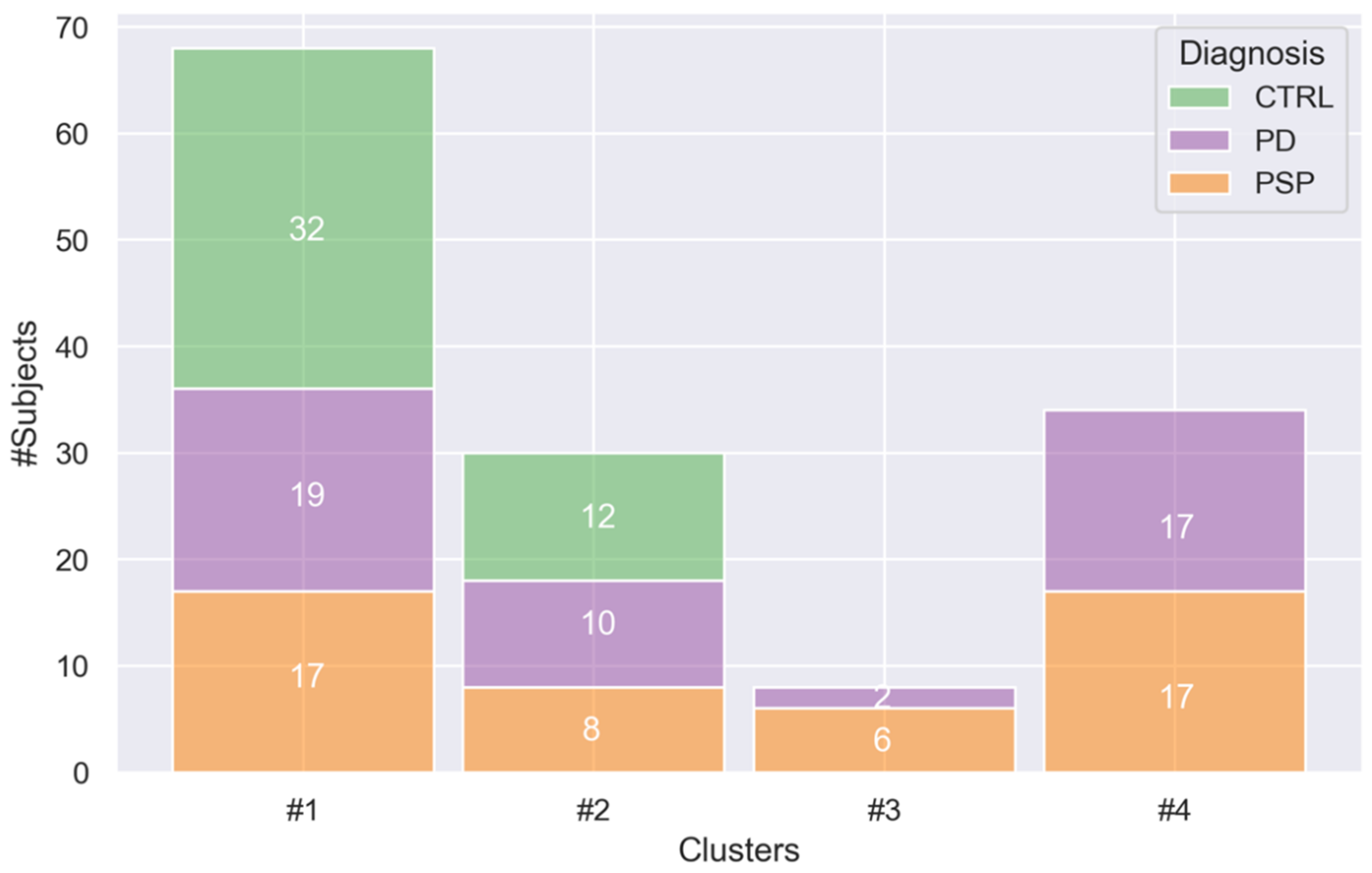
Cluster #1 was comprised of 68 participants (33 females), Cluster #2 of 30 (14 females), Cluster #3 of 8 (5 females) and Cluster #4 of 34 (17 females). Figure 5 depicted the distribution of each of the four cluster in terms of the number of CTRL participants, PD and PSP patients.

The demographic and cognitive characteristics of each cluster were shown in

Table 3. Demographic and cognitive data of the four clusters found by affinity propagation. The mean and standard deviation of the residuals of the regression with age, sex and education as covariates, are also reported in round brackets.

	Cluster #1 (68)	Cluster #2 (30)	Cluster #3 (8)	Cluster #4 (34)	p-Value	Post-Hoc
Age	62.4 ± 10.1	71.3 ± 9.94	70.4 ± 7.93	69.8 ± 7.64	<0.001 a	1 < 2,4 b
Female, n	33	14	5	17	N.S. c	N.A.
Education	12.1 ± 5.23	6.60 ± 3.23	5.5 ± 2.67	8.59 ± 4.99	<0.001 a	1 > 2,3,4 e
Total MMSE	27.3 ± 3.93	27.7 ± 1.95	12.6 ± 2.92	20.1 ± 3.57	<0.001 d	1 > 3,4 e 2 > 1,3,4 e 4 > 3 e
TO	4.68 ± 0.74 (0.026 ± 0.565)	4.9 ± 0.55 (0.800 ± 0.550)	1.25 ± 1.04 (−2.800 ± 0.842)	4.18 ± 0.97 (−0.099 ± 0.888)	<0.001 d	1 > 3 e 2 > 1,3,4 e 4 > 3 e
OS	4.71 ± 0.69 (0.067 ± 0.472)	4.83 ± 0.46 (0.856 ± 0.487)	2 ± 0.76 (−1.85 ± 0.43)	3.74 ± 1.24 (−0.454 ± 1.02)	<0.001 d	1 > 3,4 e 2 > 1,3,4 e 4 > 3 e
Reg	2.93 ± 0.39 (−0.056 ± 0.372)	3 ± 0 (0.108 ± 0.040)	2.75 ± 0.46 (−0.139 ± 0.472)	2.97 ± 0.17 (0.049 ± 0.162)	0.016 d	2 > 1 e
AC	4.21 ± 1.33 (0.345 ± 0.636)	4.60 ± 0.72 (1.89 ± 0.619)	0.50 ± 0.76 (−2.06 ± 1.11)	1.21 ± 0.99 (−1.88 ± 0.767)	<0.001 d	1 > 3,4 e 2 > 1,3,4 e
Rec	2.59 ± 0.69 (0.3 ± 0.637)	2.50 ± 0.73 (0.021 ± 0.18)	1.13 ± 0.83 (−0.775 ± 0.993)	1.09 ± 0.93 (−0.937 ± 0.889)	<0.001 d	1 > 3,4 e 2 > 3,4 e
N	2 ± 0 (0.007 ± 0.050)	1.97 ± 0.183 (0.056 ± 0.302)	1.75 ± 0.71 (−0.173 ± 0.675)	1.97 ± 0.17 (0.008 ± 0.16)	N.S. d	N.A.
SR	0.89 ± 0.31 (0.005 ± 0.300)	0.9 ± 0.30 (0.072 ± 0.532)	0.50 ± 0.53 (−0.337 ± 0.535)	0.88 ± 0.33 (0.019 ± 0.331)	0.025 d	3 < 1,2,4 e
P	2.94 ± 0.29 (−0.007 ± 0.268)	2.90 ± 0.55 (0.201 ± 0.484)	2.50 ± 0.76 (−0.312 ± 0.748)	2.88 ± 0.41 (0.024 ± 0.416)	N.S.d	N.A.
W	0.74 ± 0.41 (0.061 ± 0.316)	0.67 ± 0.479 (0.218 ± 0.38)	0.12 ± 0.35 (−0.333 ± 0.386)	0.32 ± 0.47 (−0.22 ± 0.437)	<0.001 d	1 > 3,4 e 2 > 3,4 e
CE	0.76 ± 0.43 (−0.039 ± 0.376)	0.83 ± 0.379 (0.178 ± 0.45)	0 ± 0 (−0.605 ± 0.075)	0.71 ± 0.46 (0.029 ± 0.418)	<0.001 d	1 > 3 e 2 > 1,3 e 4 > 3 e
D	0.79 ± 0.41 (0.070 ± 0.297)	0.57 ± 0.50 (0.178 ± 0.450)	0 ± 0 (−0.358 ± 0.212)	0.26 ± 0.45 (−0.213 ± 0.402)	<0.001 d	1 > 3,4 e 2 > 3,4 e

^a ANOVA p-value, significant at p < 0.05. ^b Post-hoc of ANOVA corrected for multiple comparisons with Tukey’s, significant at p < 0.05. ^c Pairwise Chi-squared, significant at p < 0.05. ^d ANCOVA with age, sex and education in covariates, significant at p < 0.05. ^e Post-Hoc of ANCOVA with age, sex and education in covariates, corrected for multiple comparisons with Tukey’s HSD test, significant at p < 0.05. Abbreviation: N.S. = not significant; N.A. = not applicable; CTRL = healthy control; PD = Parkinson’s disease patients; PSP = Progressive Supranuclear Palsy patients; TO = temporal orientation; OS = orientation in space, Reg = registration of three words; AC = attention and calculation; Rec = recall of three words; N = object naming; SR = sentence repetition; P = praxis; W = writing a sentence; CE = reading a sentence and close your eyes; D = copy a drawing.

, together with the results of statistical analyses and pairwise post-hoc results. The four clusters did not differ in the sex distribution, while Cluster #1 was younger and with the highest level of education than the other three clusters and comprised the highest number of CTRL (32). Moreover, Cluster #3 and #4 did not include any CTRL participant, but only PD and PSP patients.

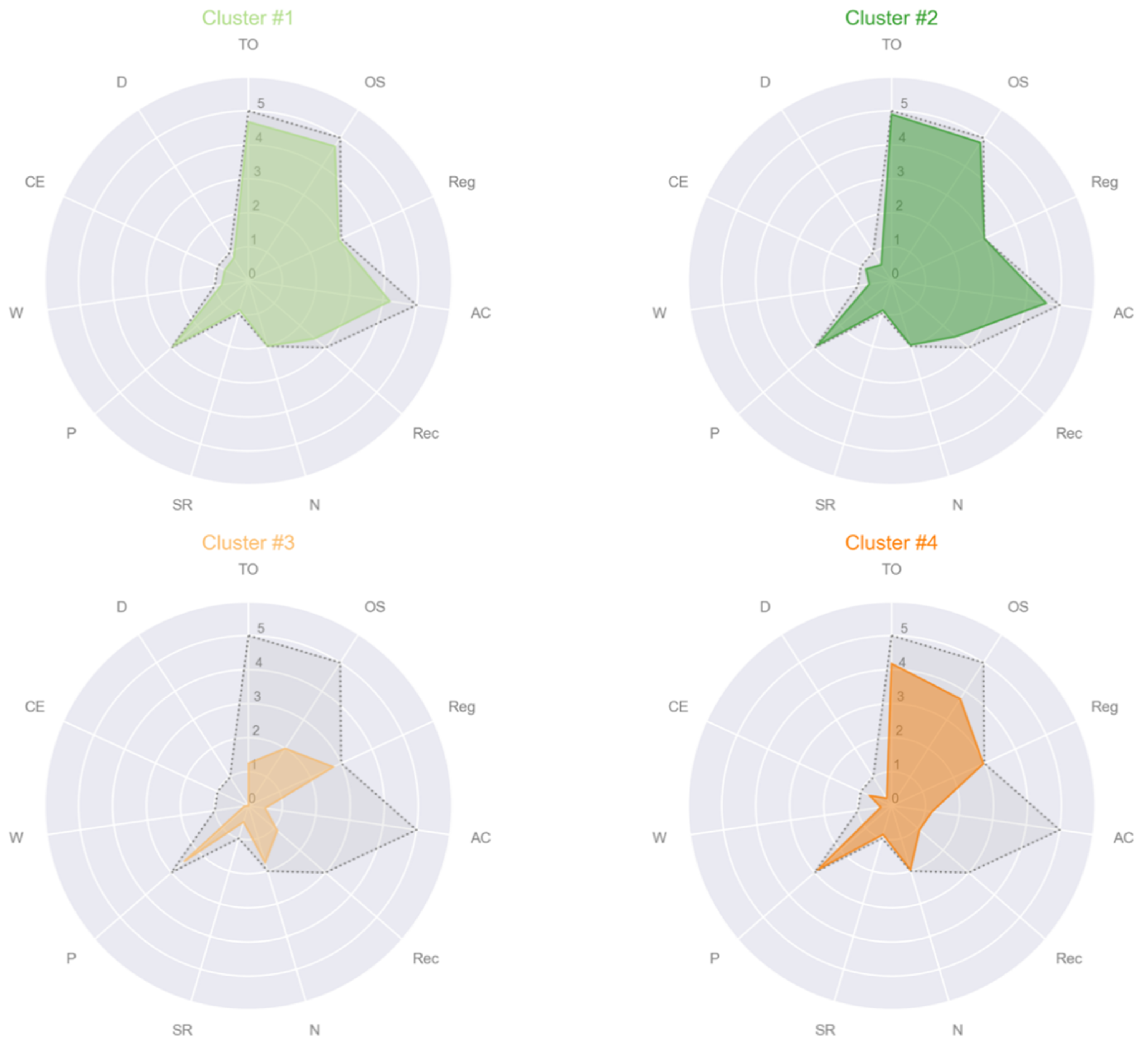
Only two MMSE subscales were not different among clusters, which is object naming (N) and the praxis (P). Cluster #3 had the lowest MMSE total score and the worst scores in all the MMSE subscales—except for the two above mentioned equal among clusters (Figure 6 for the radar plots of the four clusters). In particular, Cluster #3 had lower scores than Cluster #1 and Cluster #2 in TO, OS, AC, Rec, SR, W, CE and D and lower scores than Cluster #4 in TO, OS, SR and CE. Clusters #1 and #2 showed preserved cognitive functions in most MMSE subscales, although Cluster #2 had significant slightly higher scores than Cluster #1 in TO, OS, Reg, AC and CE.

4. Discussion

In the present study, we proposed a novel method for discovering the natural structure of cognitive impairment in Parkinsonisms patients according to the eleven MMSE subscale scores. Our application of the affinity propagation clustering algorithm on the regression residuals revealed the presence of four clusters, where two clusters (#1 and #2) showed almost intact cognitive performance, one cluster (#4) had a moderate cognitive impairment, and the last cluster (#3) had a more extensive cognitive deficit. An important finding of our work was the existence of variable levels of cognitive impairment in PD and PSP patients, showing an intra- and inter-diagnostic heterogeneity of their cognitive profiles, never investigated accurately before now with an advanced unsupervised learning technique.

Clustering was widely applied in the neuropsychology realm [10] and a variety of algorithms was used [8,9] for exploring for example, the cognitive dysfunction in Bipolar and Major Depression [11,13] or affective and psychotic disorder [12,14]. Interestingly, the findings of several works [11,12,13,14,15] showed distinct neurocognitive clusters independent from the diagnosis, as we found in our cohort of PD and PSP patients. Similarly to our results, Cotrena et al. [11] and Lewandowski et al. [14] found one neuropsychological intact subgroup (Cluster #2 in our case), one to three “intermediate” clusters (Clusters #1 and #4 in our case) and one cluster with a significant cognitive deficit (Cluster #3 of the present study), by applying both the Ward’s linkage with squared Euclidean distance. Cluster analysis with the Ward’s method was also used by Phillips et al. [16], which found heterogeneous patterns in the neurocognitive profile of early-onset Alzheimer’s patients, as indeed we found in our cohort of Parkinsonisms patients.

Although a plethora of works [18,19,20,21,22,23,24] investigated the heterogeneity among PD patients studying both motor and non-motor symptoms with clustering approaches, no one before us, explored the MMSE subscale scores, and moreover, no previous work studied the cognitive patterns of PSP patients with an unsupervised learning methodology. Indeed, a very recent work by our research group [36] already highlighted the importance of the machine learning for the evaluation of the neuropsychological and cognitive profile of PD and PSP subtypes, which could present overlapping cognitive deficits.

It is worth of noting that, as far as we know, only one previous work applied clustering on the MMSE subscales [15]. In particular, Kim et al. [15] used a two-step cluster analysis, comprised of a first phase consisting in pre-clustering and a second phase of a modified hierarchical agglomerative clustering [15] on the Korean version of the MMSE. The findings of Kim et al. [15] showed that the cluster analysis of the MMSE could be considered a reliable screening tool for the cognitive impairment of the neurodegenerative diseases, especially when complex neuropsychological batteries are not feasible.

Differently from Kim et al. [15], we did not include in the cluster analysis the age and education levels, but we treated age, gender and education levels as confounding variables, for taking into account only the influence of the diagnosis on the cognitive profile of the participants. In particular, we calculated the residuals of each MMSE subscale by applying a multiple linear regression with the method ordinary least squares. The application of cluster analysis on regression residuals was previously performed by Phillips et al. [16], which used the Ward’s method for investigating the heterogeneity of early-onset Alzheimer’s disease patients. However, it has been showed that the application of traditional clustering methods, such as K-means [25], K-median and Ward’s [5], could not be suitable for every kind of data [8,49]. More in detail, it has been suggested to privilege the use of AP algorithm in presence of sparse similarity matrix [28], as it could be occurred in the cluster analysis of regression residuals of MMSE subscales, which are discrete variables with a limited range of values (0–5).

Another strength of the AP algorithm relies in the automatic detection of the cluster centers [28,29], the exemplars, which are in our case actual participants. In particular, we found that: one healthy control participant was representative of Cluster #1, the group with almost intact cognitive profile; one PD patient relatively young and with high education level was the center of Cluster #2, the group with the most intact cognitive profile; one PD patient, elder and with low education level, was the exemplar of Cluster #3, the most cognitively impaired group, specifically in TO, OS, AC, Rec, SR, W, CE and D; one PSP patient, elder but with high education level, was the representative participant of Cluster #4, the ensemble with a moderate cognitive deficit. Such an automatic detection of cluster centers by the AP algorithm represents a valuable tool for the exploratory analysis of neuropsychological patterns when no a priori knowledge exists, and a full data-driven investigation is needed [8]. Moreover, the identification of actual participants as representatives of the clusters could provide to the neuropsychologists a more accurate understanding of the natural structure of the collected data.

As further novel contribution, our work compared the findings of the cluster analysis by varying the preference value of the AP algorithm as the median and the minimum value of the similarity matrix. Interestingly, we corroborated the literature [8,46] by finding that the use of the median dramatically overestimated the number of clusters, besides by obtaining poor performance as calculated with the Silhouette index [47,50].

The present study had two main limitations. The first is related to the specification of the similarity matrix calculated as the negative squared Euclidean distance. Indeed, we did not provide any insight whether the use of different distance metrics could provide different findings. The second limitation of the present work is the absence of the tuning of the damping factor, which could have indeed provided, as in the case of the first limitation, different results.

Further work needs to be done on a larger cohort of participants to assess whether our algorithm shows reliability and stability. Furthermore, future studies should include a more extensive battery of neuropsychological tests to confirm or not the heterogeneity of the cognitive profiles in PD and PSP patients.

In conclusion, we proposed a novel approach of unsupervised learning based on the application of AP clustering algorithm on the regression residuals of MMSE subscale scores for the exploration of the patterns of cognitive impairment of Parkinson’s disease and Progressive Supranuclear Palsy patients. Our findings revealed an intra- and inter-diagnostic heterogeneity never investigated before now among Parkinsonisms. The proposed unsupervised learning method could represent a new promising tool aimed at supporting the neuropsychologists in understanding the natural structure of MMSE performance in the neurodegenerative diseases.

References

- Tryon, R.C. Cluster analysis. Edwards Brothers. Ann. Arbor Mich. 1939, 122. [Google Scholar]
- Le, N.Q.K.; Do, D.T.; Chiu, F.Y.; Yapp, E.K.Y.; Yeh, H.Y.; Chen, C.Y. XGBoost Improves Classification of MGMT Promoter Methylation Status in IDH1 Wildtype Glioblastoma. J. Pers. Med. 2020, 10, 128. [Google Scholar] [CrossRef]
- Ho Thanh Lam, L.; Le, N.H.; Van Tuan, L.; Tran Ban, H.; Nguyen Khanh Hung, T.; Nguyen, N.T.K.; Huu Dang, L.; Le, N.Q.K. Machine Learning Model for Identifying Antioxidant Proteins Using Features Calculated from Primary Sequences. Biology 2020, 9, 325. [Google Scholar] [CrossRef]
- Johnson, S.C. Hierarchical clustering schemes. Psychometrika 1967, 32, 241–254. [Google Scholar] [CrossRef]
- Ward, J.H., Jr. Hierarchical grouping to optimize an objective function. J. Am. Stat. Assoc. 1963, 58, 236–244. [Google Scholar] [CrossRef]
- Rao, M. Cluster analysis and mathematical programming. J. Am. Stat. Assoc. 1971, 66, 622–626. [Google Scholar] [CrossRef]
- Steinhaus, H. Sur la division des corp materiels en parties. Bull. Acad. Pol. Sci. 1956, 1, 801. [Google Scholar]
- Brusco, M.J.; Steinley, D.; Stevens, J.; Cradit, J.D. Affinity propagation: An exemplar-based tool for clustering in psychological research. Br. J. Math. Stat. Psychol. 2019, 72, 155–182. [Google Scholar] [CrossRef] [PubMed] [Green Version]
- Allen, D.N.; Goldstein, G. Cluster Analysis in Neuropsychological Research; Springer: Berlin/Heidelberg, Germany, 2013. [Google Scholar]
- Morris, R.; Blashfield, R.; Satz, P. Neuropsychology and cluster analysis: Potentials and problems. J. Clin. Exp. Neuropsychol. 1981, 3, 79–99. [Google Scholar] [CrossRef]
- Cotrena, C.; Damiani Branco, L.; Ponsoni, A.; Milman Shansis, F.; Paz Fonseca, R. Neuropsychological Clustering in Bipolar and Major Depressive Disorder. J. Int. Neuropsychol. Soc. 2017, 23, 584–593. [Google Scholar] [CrossRef] [PubMed]
- Hermens, D.F.; Hodge, M.A.R.; Naismith, S.L.; Kaur, M.; Scott, E.; Hickie, I.B. Neuropsychological clustering highlights cognitive differences in young people presenting with depressive symptoms. J. Int. Neuropsychol. Soc. 2011, 17, 267–276. [Google Scholar] [CrossRef] [PubMed]
- Burdick, K.; Russo, M.; Frangou, S.; Mahon, K.; Braga, R.; Shanahan, M.; Malhotra, A. Empirical evidence for discrete neurocognitive subgroups in bipolar disorder: Clinical implications. Psychol. Med. 2014, 44, 3083. [Google Scholar] [CrossRef] [Green Version]
- Lewandowski, K.; Sperry, S.; Cohen, B.; Öngür, D. Cognitive variability in psychotic disorders: A cross-diagnostic cluster analysis. Psychol. Med. 2014, 44, 3239. [Google Scholar] [CrossRef] [Green Version]
- Kim, S.Y.; Lim, T.S.; Lee, H.Y.; Moon, S.Y. Clustering mild cognitive impairment by mini-mental state examination. Neurol. Sci. 2014, 35, 1353–1358. [Google Scholar] [CrossRef] [PubMed]
- Phillips, M.L.; Stage, E.C., Jr.; Lane, K.A.; Gao, S.; Risacher, S.L.; Goukasian, N.; Saykin, A.J.; Carrillo, M.C.; Dickerson, B.C.; Rabinovici, G.D.; et al. Neurodegenerative Patterns of Cognitive Clusters of Early-Onset Alzheimer’s Disease Subjects: Evidence for Disease Heterogeneity. Dement. Geriatr. Cogn. Disord. 2019, 48, 131–142. [Google Scholar] [CrossRef] [PubMed]
- Alashwal, H.; El Halaby, M.; Crouse, J.J.; Abdalla, A.; Moustafa, A.A. The Application of Unsupervised Clustering Methods to Alzheimer’s disease. Front. Comput. Neurosci. 2019, 13, 31. [Google Scholar] [CrossRef] [PubMed]
- Van Rooden, S.M.; Heiser, W.J.; Kok, J.N.; Verbaan, D.; Van Hilten, J.J.; Marinus, J. The identification of Parkinson’s disease subtypes using cluster analysis: A systematic review. Mov. Disord. 2010, 25, 969–978. [Google Scholar] [CrossRef]
- Mu, J.; Chaudhuri, K.R.; Bielza, C.; de Pedro-Cuesta, J.; Larrañaga, P.; Martinez-Martin, P. Parkinson’s Disease Subtypes Identified from Cluster Analysis of Motor and Non-motor Symptoms. Front. Aging Neurosci. 2017, 9. [Google Scholar] [CrossRef]
- Liu, P.; Feng, T.; Wang, Y.-j.; Zhang, X.; Chen, B. Clinical heterogeneity in patients with early-stage Parkinson’s disease: A cluster analysis. J. Zhejiang Univ. Sci. B 2011, 12, 694. [Google Scholar] [CrossRef]
- van Rooden, S.M.; Colas, F.; Martinez-Martin, P.; Visser, M.; Verbaan, D.; Marinus, J.; Chaudhuri, R.K.; Kok, J.N.; van Hilten, J.J. Clinical subtypes of Parkinson’s disease. Mov. Disord. 2011, 26, 51–58. [Google Scholar] [CrossRef]
- Erro, R.; Vitale, C.; Amboni, M.; Picillo, M.; Moccia, M.; Longo, K.; Santangelo, G.; De Rosa, A.; Allocca, R.; Giordano, F.; et al. The heterogeneity of early Parkinson’s disease: A cluster analysis on newly diagnosed untreated patients. PLoS ONE 2013, 8, e70244. [Google Scholar] [CrossRef]
- Ma, L.Y.; Chan, P.; Gu, Z.Q.; Li, F.F.; Feng, T. Heterogeneity among patients with Parkinson’s disease: Cluster analysis and genetic association. J. Neurol. Sci. 2015, 351, 41–45. [Google Scholar] [CrossRef]
- Pont-Sunyer, C.; Hotter, A.; Gaig, C.; Seppi, K.; Compta, Y.; Katzenschlager, R.; Mas, N.; Hofeneder, D.; Brücke, T.; Bayés, A. The Onset of Nonmotor Symptoms in Parkinson’s disease (The ONSET PD S tudy). Mov. Disord. 2015, 30, 229–237. [Google Scholar] [CrossRef]
- Jin, X.; Han, J. K-Means Clustering; Springer: Berlin/Heidelberg, Germany, 2010. [Google Scholar]
- Steinley, D.; Brusco, M.J. Evaluating mixture modeling for clustering: Recommendations and cautions. Psychol. Methods 2011, 16, 63. [Google Scholar] [CrossRef] [PubMed]
- Milligan, G.W.; Cooper, M.C. An examination of procedures for determining the number of clusters in a data set. Psychometrika 1985, 50, 159–179. [Google Scholar] [CrossRef]
- Frey, B.J.; Dueck, D. Clustering by passing messages between data points. Science 2007, 315, 972–976. [Google Scholar] [CrossRef] [Green Version]
- Mézard, M. Where are the exemplars? Science 2007, 315, 949–951. [Google Scholar] [CrossRef] [PubMed] [Green Version]
- Thavikulwat, P. Affinity Propagation: A Clustering Algorithm for Computer-Assisted Business Simulations and Experiential Exercises. Available online: http://citeseerx.ist.psu.edu/viewdoc/download?doi=10.1.1.490.7628&rep=rep1&type=pdf (accessed on 3 February 2021).
- Hoglinger, G.U.; Respondek, G.; Stamelou, M.; Kurz, C.; Josephs, K.A.; Lang, A.E.; Mollenhauer, B.; Muller, U.; Nilsson, C.; Whitwell, J.L.; et al. Clinical diagnosis of progressive supranuclear palsy: The movement disorder society criteria. Mov. Disord. 2017, 32, 853–864. [Google Scholar] [CrossRef]
- Quattrone, A.; Morelli, M.; Nigro, S.; Quattrone, A.; Vescio, B.; Arabia, G.; Nicoletti, G.; Nistico, R.; Salsone, M.; Novellino, F.; et al. A new MR imaging index for differentiation of progressive supranuclear palsy-parkinsonism from Parkinson’s disease. Parkinsonism Relat. Disord. 2018, 54, 3–8. [Google Scholar] [CrossRef] [PubMed]
- Barbagallo, G.; Morelli, M.; Quattrone, A.; Chiriaco, C.; Vaccaro, M.G.; Gulla, D.; Rocca, F.; Caracciolo, M.; Novellino, F.; Sarica, A.; et al. In vivo evidence for decreased scyllo-inositol levels in the supplementary motor area of patients with Progressive Supranuclear Palsy: A proton MR spectroscopy study. Parkinsonism Relat. Disord. 2019, 62, 185–191. [Google Scholar] [CrossRef] [PubMed]
- Goldman, J.G.; Holden, S.K.; Litvan, I.; McKeith, I.; Stebbins, G.T.; Taylor, J.P. Evolution of diagnostic criteria and assessments for Parkinson’s disease mild cognitive impairment. Mov. Disord. 2018, 33, 503–510. [Google Scholar] [CrossRef] [Green Version]
- Postuma, R.B.; Berg, D.; Stern, M.; Poewe, W.; Olanow, C.W.; Oertel, W.; Obeso, J.; Marek, K.; Litvan, I.; Lang, A.E.; et al. MDS clinical diagnostic criteria for Parkinson’s disease. Mov. Disord. 2015, 30, 1591–1601. [Google Scholar] [CrossRef]
- Vaccaro, M.G.; Sarica, A.; Quattrone, A.; Chiriaco, C.; Salsone, M.; Morelli, M.; Quattrone, A. Neuropsychological assessment could distinguish among different clinical phenotypes of progressive supranuclear palsy: A Machine Learning approach. J. Neuropsychol. 2020. [Google Scholar] [CrossRef] [PubMed]
- Carpinelli Mazzi, M.; Iavarone, A.; Russo, G.; Musella, C.; Milan, G.; D’Anna, F.; Garofalo, E.; Chieffi, S.; Sannino, M.; Illario, M.; et al. Mini-Mental State Examination: New normative values on subjects in Southern Italy. Aging Clin. Exp. Res. 2020, 32, 699–702. [Google Scholar] [CrossRef] [PubMed]
- Folstein, M.F.; Folstein, S.E.; McHugh, P.R. “Mini-mental state”. A practical method for grading the cognitive state of patients for the clinician. J. Psychiatr. Res. 1975, 12, 189–198. [Google Scholar] [CrossRef]
- Grigoletto, F.; Zappalà, G.; Anderson, D.W.; Lebowitz, B.D. Norms for the Mini-Mental State Examination in a healthy population. Neurology 1999, 53, 315. [Google Scholar] [CrossRef]
- Pedregosa, F.; Varoquaux, G.; Gramfort, A.; Michel, V.; Thirion, B.; Grisel, O.; Blondel, M.; Prettenhofer, P.; Weiss, R.; Dubourg, V. Scikit-learn: Machine learning in Python. J. Mach. Learn. Res. 2011, 12, 2825–2830. [Google Scholar]
- Harris, C.R.; Millman, K.J.; van der Walt, S.J.; Gommers, R.; Virtanen, P.; Cournapeau, D.; Wieser, E.; Taylor, J.; Berg, S.; Smith, N.J. Array programming with NumPy. Nature 2020, 585, 357–362. [Google Scholar] [CrossRef] [PubMed]
- Hunter, J.D. Matplotlib: A 2D graphics environment. Comput. Sci. Eng. 2007, 9, 90–95. [Google Scholar] [CrossRef]
- McKinney, W. Data structures for statistical computing in python. In Proceedings of the 9th Python in Science Conference, Austin, TX, USA, 28 June–3 July 2010; pp. 51–56. [Google Scholar]
- Seabold, S.; Perktold, J. Statsmodels: Econometric and statistical modeling with python. In Proceedings of the 9th Python in Science Conference, Austin, TX, USA, 28 June–3 July 2010; p. 61. [Google Scholar]
- Hutcheson, G.D. Ordinary least-squares regression. In L. Moutinho and GD Hutcheson, the SAGE Dictionary of Quantitative Management Research; Sage: Southend Oaks, CA, USA, 2011; pp. 224–228. [Google Scholar]
- Brusco, M.J.; Köhn, H.-F. Exemplar-based clustering via simulated annealing. Psychometrika 2009, 74, 457–475. [Google Scholar] [CrossRef]
- Rousseeuw, P.J. Silhouettes: A graphical aid to the interpretation and validation of cluster analysis. J. Comput. Appl. Math. 1987, 20, 53–65. [Google Scholar] [CrossRef] [Green Version]
- Dueck, D. Affinity Propagation: Clustering Data by Passing Messages. Ph.D. Thesis, University of Toronto, Toronto, ON, Canada, September 2009. [Google Scholar]
- Brusco, M.J.; Shireman, E.; Steinley, D. A comparison of latent class, K-means, and K-median methods for clustering dichotomous data. Psychol. Methods 2017, 22, 563–580. [Google Scholar] [CrossRef] [PubMed]
- Starczewski, A. A new validity index for crisp clusters. Pattern Anal. Appl. 2017, 20, 687–700. [Google Scholar] [CrossRef] [Green Version]
Figure 1.
Schematic representation of the functioning of the affinity propagation algorithm in a 3D fashion. Figure adapted and revised from Frey and Dueck [28].
Figure 2.
Radar plots of the mean of the eleven Mini Mental State Examination (MMSE) subscales per diagnosis: healthy controls (CTRL), Parkinson’s disease patients (PD) and Progressive Supranuclear Palsy patients (PSP). In gray and dotted lines the maximum value that each MMSE subscale could reach: Max(TO) = 5, Max(OS) = 5, Max(Reg) = 3, Max(AC) = 5, Max(Rec) = 3, Max(N) = 2, Max(SR) = 1, Max(P) = 3, Max(W) = 1, Max(CE) = 1, Max(D) = 1. Abbreviations: CTRL = healthy control; PD = Parkinson’s disease patients; PSP = Progressive Supranuclear Palsy patients; TO = temporal orientation; OS = orientation in space, Reg = registration of three words; AC = attention and calculation; Rec = recall of three words; N = object naming; SR = sentence repetition; P = praxis; W = writing a sentence; CE = reading a sentence and close your eyes; D = copy a drawing.
Figure 3.
Radar plots of the mean of the eleven MMSE subscales per cluster of Parkinson’s disease (PD) patients. In gray and dotted lines the maximum value that each MMSE subscale could reach: Max(TO) = 5, Max(OS) = 5, Max(Reg) = 3, Max(AC) = 5, Max(Rec) = 3, Max(N) = 2, Max(SR) = 1, Max(P) = 3, Max(W) = 1, Max(CE) = 1, Max(D) = 1. Abbreviations: TO = temporal orientation; OS = orientation in space, Reg = registration of three words; AC = attention and calculation; Rec = recall of three words; N = object naming; SR = sentence repetition; P = praxis; W = writing a sentence; CE = reading a sentence and close your eyes; D = copy a drawing.
Figure 4.
Radar plots of the mean of the eleven MMSE subscales per cluster of Progressive Supranuclear Palsy (PSP) patients. In gray and dotted lines the maximum value that each MMSE subscale could reach: Max(TO) = 5, Max(OS) = 5, Max(Reg) = 3, Max(AC) = 5, Max(Rec) = 3, Max(N) = 2, Max(SR) = 1, Max(P) = 3, Max(W) = 1, Max(CE) = 1, Max(D) = 1. Abbreviations: TO = temporal orientation; OS = orientation in space, Reg = registration of three words; AC = attention and calculation; Rec = recall of three words; N = object naming; SR = sentence repetition; P = praxis; W = writing a sentence; CE = reading a sentence and close your eyes; D = copy a drawing.
Figure 5.
Distribution of diagnoses among the four clusters found by affinity propagation. Cluster #1 consisted of 32 CTRL, 19 PD and 17 PSP. Cluster #2 consisted of 12 CTRL, 10 PD and 8 PSP. Cluster #3 consisted of 2 PD and 6 PSP. Cluster #4 consisted of 17 PD and 17 PSP. Abbreviations: CTRL = healthy control; PD = Parkinson’s disease patients; PSP = Progressive Supranuclear Palsy patients.
Figure 6.
Radar plots of the mean of the eleven MMSE subscales per cluster. In gray and dotted lines the maximum value that each MMSE subscale could reach: Max(TO) = 5, Max(OS) = 5, Max(Reg) = 3, Max(AC) = 5, Max(Rec) = 3, Max(N) = 2, Max(SR) = 1, Max(P) = 3, Max(W) = 1, Max(CE) = 1, Max(D) = 1. Abbreviations: TO = temporal orientation; OS = orientation in space, Reg = registration of three words; AC = attention and calculation; Rec = recall of three words; N = object naming; SR = sentence repetition; P = praxis; W = writing a sentence; CE = reading a sentence and close your eyes; D = copy a drawing.