
Optimization Method of Customized Shuttle Bus Lines under Random Condition

1
China Academy of Transportation Sciences, Beijing 100029, China
2
MOE Key Laboratory for Urban Transportation Complex Systems Theory and Technology, Beijing Jiaotong University, Beijing 100044, China
*
Author to whom correspondence should be addressed.
Algorithms 2021, 14(2), 52; https://0-doi-org.brum.beds.ac.uk/10.3390/a14020052
Submission received: 18 December 2020
/
Revised: 29 January 2021
/
Accepted: 2 February 2021
/
Published: 5 February 2021
Abstract
:Transit network optimization can effectively improve transit efficiency, improve traffic conditions, and reduce the pollution of the environment. In order to better meet the travel demands of passengers, the factors influencing passengers’ satisfaction with a customized bus are fully analyzed. Taking the minimum operating cost of the enterprise as the objective and considering the random travel time constraints of passengers, the customized bus routes are optimized. The K-means clustering analysis is used to classify the passengers’ needs based on the analysis of the passenger travel demand of the customized shuttle bus, and the time stochastic uncertainty under the operating environment of the customized shuttle bus line is fully considered. On the basis of meeting the passenger travel time requirements and minimizing the cost of service operation, an optimization model that maximizes the overall satisfaction of passengers and public transit enterprises is structured. The smaller the value of the objective function is, the lower the operating cost. When the value is negative, it means there is profit. The model is processed by the deterministic processing method of random constraints, and then the hybrid intelligent algorithm is used to solve the model. A stochastic simulation technique is used to train stochastic constraints to approximate uncertain functions. Then, the improved immune clonal algorithm is used to solve the vehicle routing problem. Finally, it is proved by a case that the method can reasonably and efficiently realize the optimization of the customized shuttle bus lines in the region.
1. Introduction
In recent years, as a special mode of public transport, a customized shuttle bus has been increasingly popular. Taking Beijing as an example, the daily average passenger volume of customized buses (business buses, high-speed rail lines, leisure tourism lines, etc.) has reached 37,000. A customized shuttle bus is a public transit mode, serving the individual demands for the passengers whose origins and destinations, travel time, and service level requirement is similar. A customized shuttle bus is an important part of urban public transit. The stops (including transfer stops) and routes of customized shuttle bus are set up according to the individual demands. The ticket fare of customized shuttle bus is higher than one of the bus and subway, but is lower than one of the self-driving and taxi. Passengers usually need to pay a ticket fare in advance in months or weeks. A customized shuttle bus can provide door-to-door service and seat for each passenger. Moreover, WIFI, travel information search, and multimedia are available to passengers. Locations of stops are determined according to demands. The stops can be specialized or bus stops. The routes of the customized shuttle bus can be fixed or adjusted according to the traffic conditions. However, the stop coverage must meet the demands. Related research results showed that four factors can influence passengers’ willingness to choose a customized shuttle bus: Private car, distance between the home and work place, travel satisfaction level, and work overtime [1].
To reflect the advantages of customized shuttle bus, especially the accuracy of travel time, the routes of vehicles should be optimized reasonably. Route optimization or scheduling optimization of the customized shuttle bus or a similar service have been studied by a few papers. Lei et al. (2017) used the K-means clustering analysis to cluster real-time demands of residents, and a dynamic scheduling model was developed with the maximal demand service rate and minimum cost as the objectives and the maximal capacity and passenger time threshold factors as the constraints. Then, a parallel ant colony algorithm based on the Hadoop platform was proposed [2]. Cheng (2014) studied the layout of the customized shuttle bus with the level analysis method of point, line, and plane [3]. To design the service area and routing for a flexible feeder transit system, Pan et al. (2014) presented a mathematical model with objectives to maximize the number of served passengers and minimize the operational cost [4]. A route planning and coordinated scheduling model was developed by Pan et al. (2016) to minimize passengers’ cost and operator cost [5].
For similarities between the customized shuttle bus and common public transit, the line optimization method for a common public transit can be used for reference when the characteristics of the customized shuttle bus are fully considered. Lin et al. (1999) presented a nonlinear 0–1 programming model for the bus network design problem from the viewpoint of a combination of optimization and minimizing of passengers travel time and operation cost of the bus network. The stop capacity is taken into account and the simulated annealing algorithm was adopted to solve the model [6]. Zhou and Luo (2013) established a layout bi-level optimization model of a comprehensive transit system and an algorithm based on improved IOA was proposed, which overcame the defects of a lack of significant hierarchy and improved solve efficiency [7]. He and Fan (2007) considered the impacts of transfer times, transfer point choice, and travel cost on solving the optimal path. The transfer walk-time matrix was constructed and a multiplication of the transfer matrix was transformed to the addition of the transfer walk-time matrix and public traffic travel-time matrix [8]. Mireia R.R. et al. (2012) proposed a bilevel formulation for solving the Bus Network Design Problem (BNDP) of interurban services entering a major city. The objective function of the first level was defined with the aim of reducing the user and agency costs. In the second level, the performance of users was addressed. Furthermore, a local search method based on the Tabu search algorithm was carried out to guide the exploration in the solution domain [9]. Perugia A. et al. (2012) presented a model and an algorithm for the design of a home-to-work bus service in a metropolitan area. A multiobjective model was introduced, among other aspects, equity was considered by time windows on the arrival time of a bus at a stop. In addition, a cluster routing approach was proposed to model both the bus stop location and routing in urban road networks where turn restrictions exist. The resulting multi-objective location-routing model was solved by a Tabu search algorithm [10]. Amiripour S.M.M. et al. (2014) based on the analysis of seasonal transit demand variations, studied the design of the bus network. In order to solve this NP hard problem, a genetic algorithm-based method was proposed. The optimization was realized by a defined objective function [11]. Leksakul et al. (2017) compared solution methods for different location-routing problems and the optimal route between 300–700 bus stops allocated by the K-means clustering analysis was determined with the ant colony optimization [12]. A methodological framework was formulated by Ouyang et al. (2014), and heterogeneous route configurations generated by this framework can reduce the cost of bus users and operating agency [13]. Chang and Hu (2005) proposed a linear mathematical model on the bus line network, and passengers’ travel time, public transit network density, as well as operator’s benefit were considered [14]. Tom and Mohan (2003) designed the transit route network in a two-phase solution process: A large set of the candidate route is generated in the first phase and a solution route set is selected from the candidate route set in the second phase, while the bus operating cost and passenger total travel time were minimized [15]. Wei and Machemehl (2006, 2012) considered the user cost, operator cost, and unsatisfied demand cost [16,17]. Xu et al. (2015) considered the interests of passengers and bus companies and established a bi-level programming model of public transit network planning, while the equilibrium analysis of the passenger travelling choice behavior was made based on the strategy equilibrium transit assignment [18]. Yu and Liang (2016) established an integer nonlinear programming model for designing the optimal bus transit network to minimize the total cost of the bus operation and passenger travel time [19]. A network optimization model was developed by Hu et al. (2008), and benefits maximization, costs minimization, and sustainable development were considered [20]. Yu et al. (2012) built a direct traveler density model and extended it to design the transit network, aiming to minimize the number of transfer times and maximize the demand density of the route [21]. Zhao and Zeng (2007) presented a methodology for optimizing transit networks based on both passenger and operator costs [22]. Szeto and Jiang (2014) proposed a bi-level transit network design problem and the objective of upper-level was to minimize the number of passenger transfers, while the lower-level problem was a transit assignment problem [23].
We can conclude that the objectives of works on the bus network optimization are mainly minimal travel time, cost or transfer times, while residents’ travel behavior is less considered. Among the factors affecting the optimization of customized bus routes, the most important are the travel cost and time, in which travel time often has a certain randomness. Given that stops of the customized shuttle bus are set up according to demands, this paper optimizes the customized shuttle bus network from the point of residents’ travel behavior. The remainder of this paper is organized as follows: The next section analyzes passengers’ travel demands along with the model formulation. A heuristic algorithm is proposed and illustrated in Section 3. Section 4 gives an illustrative example to demonstrate the validity of the model and effectiveness of the heuristic algorithm. The concluding remarks are made in the last section.
2. Problem Formulation
In a certain region, the customized shuttle bus travel demand data is obtained through the OD demand survey, and the alternative bus stops are determined based on the K-means clustering analysis. The objective is to minimize the difference between the operating costs and ticket revenue, and the constraint conditions are vehicle stops, passenger capacity, and operation time. The customized shuttle bus route optimization model is constructed, focusing on the time uncertainty in the process of vehicle operation, the stochastic uncertainty constraints of time are given.
2.1. Travel Demand Analysis
Passengers often choose the shortest route. In medium or small cities where the traffic condition is better, the shortest route is usually the most convenient, economical, and efficient route. However, in large cities, especially mega-cities, the shortest route often means more travel time and cost for traffic jam.
Different from the common public transit, customized shuttle bus stops are set up based on travel demand and the travel time of each route is fixed. Routes can be adjusted according to the traffic condition. Therefore, customized shuttle bus routes can be optimized by the analysis of the situation of land utilization along the route and detouring around the traffic jam.
Based on big data analytics, we adopt the K-means clustering analysis to classify passengers [24]. There is a positive integer set X = {x1, x2, …, xn} and the data in this set are divided into k subsets, C = {ck, k = 1, 2, …, N}. There is a data center μk in each subset which represents a kind of data. Euclidean distance is used as the criterion. The quadratic sum of distances between the data points and data center μk will be calculated and minimized.
Whether travel demand points will be divided into the same subset depends on whether the distances between the cluster center and origins or destinations meet passengers’ expectation which is 500 m in this paper. The cluster center of origins or destinations will be the customized shuttle bus stop.
The principle of the K-means algorithm is as follows:
Step 1: Data normalization and outlier processing;
Step 2: Randomly select k-clustering centroids (alternative bus stops);
Step 3: All data points are related and divided to the nearest centroid, and clustering is based on it;
Step 4: Move the particle to the center (means) of the current partition cluster containing all the data points;
Repeat step 2 and step 3 N times until the sum of squares of the distances from all points to their cluster centroid is the smallest.
Through the K-means clustering algorithm, the group of μk covering the most OD is selected as the candidate bus stops.
2.2. Model Establishment
Based on the candidate stations calculated by the above clustering analysis method, the following assumptions need to be considered before establishing the route optimization model and the corresponding solution method.
2.2.1. Modeling Assumption
The operation cost and travel time requirement will be considered based on a reasonable ticket fare. The optimization objective is to minimize the operation cost. To simplify the problem, the following conditions will be satisfied.
- Each depot will be analyzed alone. The vehicle type for one depot will be the same. The unit operation cost is fixed and proportional to the operation mileages.
- Each vehicle can only travel along one route while serving several stops. The trip volume of each OD at each stop will not exceed the vehicle capacity.
- The number of passengers getting on or off the bus at each stop is known in the decision period. Passengers without an appointment are not allowed to take the bus.
- The timetable will be observed strictly. A delay caused by emergencies such as accidents or disasters will be neglected.
- A single ticket fare will be adopted.
2.2.2. Notations
The following terms have been defined and commonly used in our model.
| Sets | |
| A | set of depots (departure point of vehicles), A = {i|i= 1, 2, …, n} |
| V | set of demand points (stops), V = {v|v= 1, 2, …, m} |
| B | set of vehicles, B = {b|b= 1, 2, …, k} |
| S | set of the number of stops served by vehicles, S= {s|s = 1, 2, …, m} |
| Parameters | |
| mb | the number of stops served by vehicle b, |
| Qv | the number of passengers getting on the bus at stop v |
| Pv | the number of passengers getting off the bus at stop v |
| ds | the number of passengers in the area served by stop s |
| fs | ticket fare for one passenger served by stop s |
| rb | capacity of vehicle b |
| lv | distance between the depot and demand point v |
| lu,v | length of the shortest route between stop u and stop v |
| cb | unit operation cost of a vehicle |
| fixed cost of a vehicle for one trip | |
| the number of passengers in vehicle b after the sth stop served | |
| the time when the vehicle b starts from the depot | |
| vehicle b running time from stop u to stop v | |
| bus arrival time required by stop v | |
| Lb | distance between the depot and first stop served by vehicle b, |
| distance between the first stop and last stop served by vehicle b, | |
| The time when vehicle b reaches stop v | |
| Decision variables | |
| 0–1 if or not the sth stop served by vehicle b is stop v | |
2.2.3. Mathematical Formulation
We aim at deciding routes of vehicles reasonably to meet demands while the number of stops served by each vehicle is unknown. The optimization objective is to minimize the operation cost of all vehicles under a vehicle capacity constraint.
Based on the above, we now introduce the objectives and constraints.
s.t.
The objective function (4) minimizes the cost of all the vehicles. Constraint (5) means that each vehicle cannot serve more than one stop simultaneously. Constraint (6) ensures that each stop can only be served once for each vehicle in one trip. Constraint (7)–(10) are the vehicle capacity constraints. Constraint (7) represents the number of passengers at the first stop in each vehicle. Constraint (8) indicates the number of passengers aboard when the vehicles departure from the second stop. Constraint (9) is the recursion formula to calculate the number of passengers in each vehicle at each stop. Constraint (10) sets the limit of the number of passengers in each vehicle. Constraint (11)–(14) are time constraints. Constraint (11) states the departure time of each vehicle. Constraint (12) represents when each vehicle arrives at the first stop served. Constraint (13) indicates when each vehicle arrives at other stops served. Constraint (14) states the uncertainty for vehicles’ arrival time at stops. and are the definitions of positive and negative deviation of arrival time at stop v for vehicle b, respectively.
3. Solution Algorithm
We will try to guarantee that the probability that the vehicle’s arrive stop v within the specified time is not less than βv. Constraint (14) can be transferred to a chance constraint (Liu et al. 2003) [25].
The prominent feature of the programming model with a stochastic chance constraint is that the decision-maker is allowed to make a decision that does not meet the constraint conditions to a certain extent, but the probability of the constraint conditions is not less than a certain confidence level. The neural network has a strong nonlinear approximation function, and its approximation ability for complex objects with uncertainty is better than any previous method based on the accurate mathematical model. It has been proven that the neural network with a deviation and at least one S-type hidden layer plus a linear output layer can approximate any rational function. Therefore, this manuscript uses the neural network to realize the approximation of the random function. In the process of algorithm implementation, the neural network can be used to approximate the random function to reduce the amount of calculation and speed up the solution process. It is feasible to use the trained neural network to calculate the random function. The trained neural network is nested in the immune clonal algorithm, and the optimal solution is obtained by using the search performance of the immune clonal algorithm.
We propose a hybrid intelligent optimization algorithm based on the immune clone algorithm, stochastic simulation technique, and neural network. The algorithm works as follows:
| Step 1 |
| Generate input and output data of the uncertain function (15) with the stochastic simulation technique. |
| Step 2 |
| A neural network is trained to approximate the uncertain function from the input and output data generated in Step 1. |
| Step 3 |
| Create the initial population and the feasibility of antibodies will be checked with the neural network. |
| Step 4 |
| Update antibodies by a clone operator and immune genic operator and the feasibility of child antibodies will be checked with the neural network. |
| Step 5 |
| Calculate all antibodies’ objective values with the neural network. |
| Step 6 |
| Calculate all antibodies’ affinity based on the objective values. |
| Step 7 |
| Select antibodies by the clone selection. |
| Step 8 |
| Iterate from Step 4 to 7 until the end criterion is met. |
| Step 9 |
| Output the optimal solutions. |
3.1. Antibody Coding
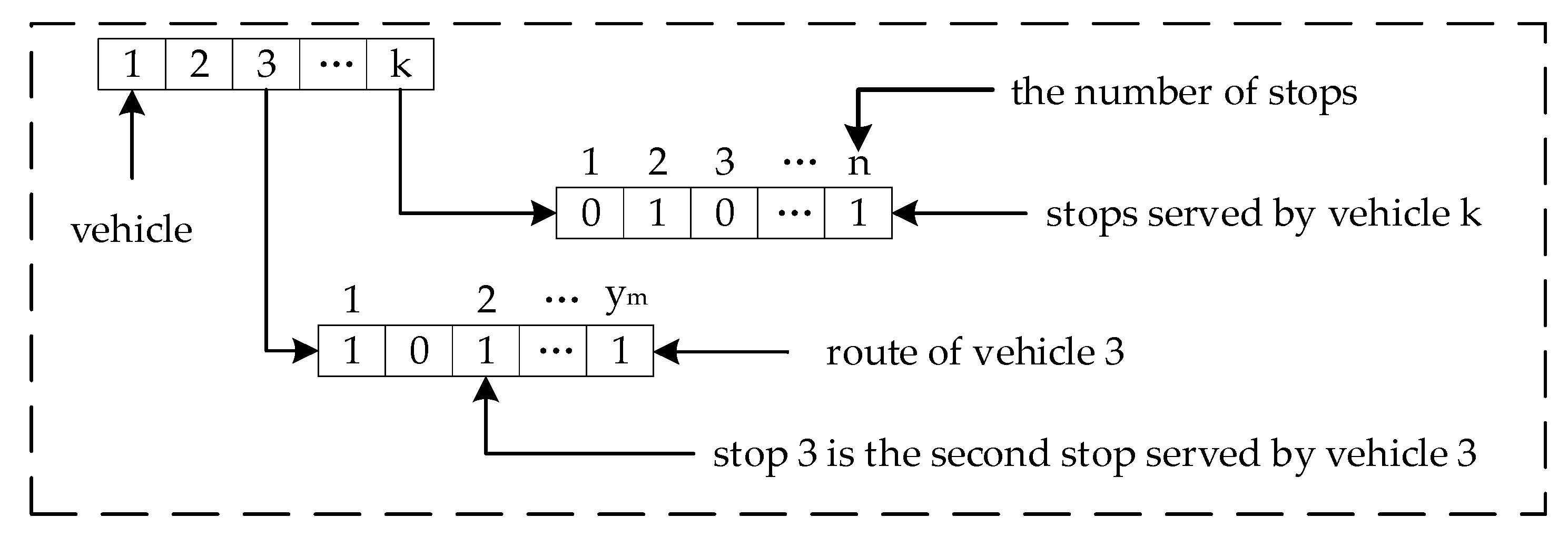
Antibody v = (x, y, t) represents a decision process and gene x = (x1, x2, x3, …, xn) represents the n stops; y = (y1, y2, y3, …, ym−1) is the number of stops served by the vehicle, and “0” is the depot; t = (t1, t2, t3, …, tb) and tb represent the departure time from the depot for vehicle b; and ym = ym−1 means that vehicle b has not departed from the depot, while ym > ym−1 means that vehicle b has departed from the depot and the departure time is tb. Schematic plot of antibody coding presented in Figure 1.
3.2. Initial Population
For gene x, we define xi = i and a series {x1, x2, x3, …, xn} is defined, I = 1, 2, 3, …, n. The following process will be repeated: Select a position n′ randomly between j and n, then exchange the values of xj and xn′ to ensure that {x1, x2, x3, …, xn} is a reset of {1, 2, 3, …, n}. Gene x = {x1, x2, x3, …, xn} will be generated.
If , generate random number yi between 0 and n, then the series will be reset from small to large and we will obtain gene y = (y1, y2, y3, …, ym−1).
For i = 1, 2, 3, …, k, we define ti is a random number for departure time a, then gene t = (t1, t2, t3, …, tk).
If antibody v = (x, y, t) is feasible, it will be accepted. Otherwise repeat the process above until a feasible antibody is generated.
3.3. Clone Operator
For the clone operator, the population V is updated to V’ as follows:
, Ii is a qi-dimension row vector of where all elements are “1”. The clone scale of antibody vi (x, y, t) should be adjusted adaptively according to its affinity to antigens and avidities to other antibodies. The clone scale should be calculated as follows:
where is a function to round up the input to an integer. nc is a set value in connection with the clone scale and nc > k. f (vi (x, y, t)) is the affinity of antibody vi (x, y, t) to the antigens. is the avidity of antibody vi (x, y, t) to other antibodies and can be calculated by Formula (18).
where is the Euclidean distance which means that . Obviously the larger the antibody’s avidities, the more the antibody is similar to other antibodies and inhibition among the antibodies is stronger.
3.4. Immune Genic Operator
Crossover
For antibodies v1 and v2, where v1 = (x1, y1, t1) and v2 = (x2, y2, t2), the crossover operator can be executed as follows: Generate a random number c in the open interval (0,1), then we define , . Child antibodies and can be obtained by the crossover operator, where ,.
Mutation
For gene x of antibody v = (x, y, t), we generate two positions n1 and n2 between 1 and n randomly for the mutation operator. Then, the series will be reset and a new series will be obtained. A new gene will be as follows:
For gene y, two positions n1 and n2 between 1 and m−1 will be generated randomly. For I = n1, n1+1, n1+2, …, n2, we define yi as a random number between 0 and n. Then, we reset the series from small to large in order to obtain a new gene y’.
For gene t, we generate a mutation direction d in Rk. If is out of the time window for a predetermined step size M, M will be set as a random number between 0 and M until the time window is met. When gene t in the time window cannot be obtained by the above process within iterations, we set M = 0. Finally, t will be replaced by child gene .
Selection operator
Combine the parent population and children as one, then select an antibody with the highest affinity to be kept to the children population, which avoids the degradation of the algorithm [26].
4. Numerical Example
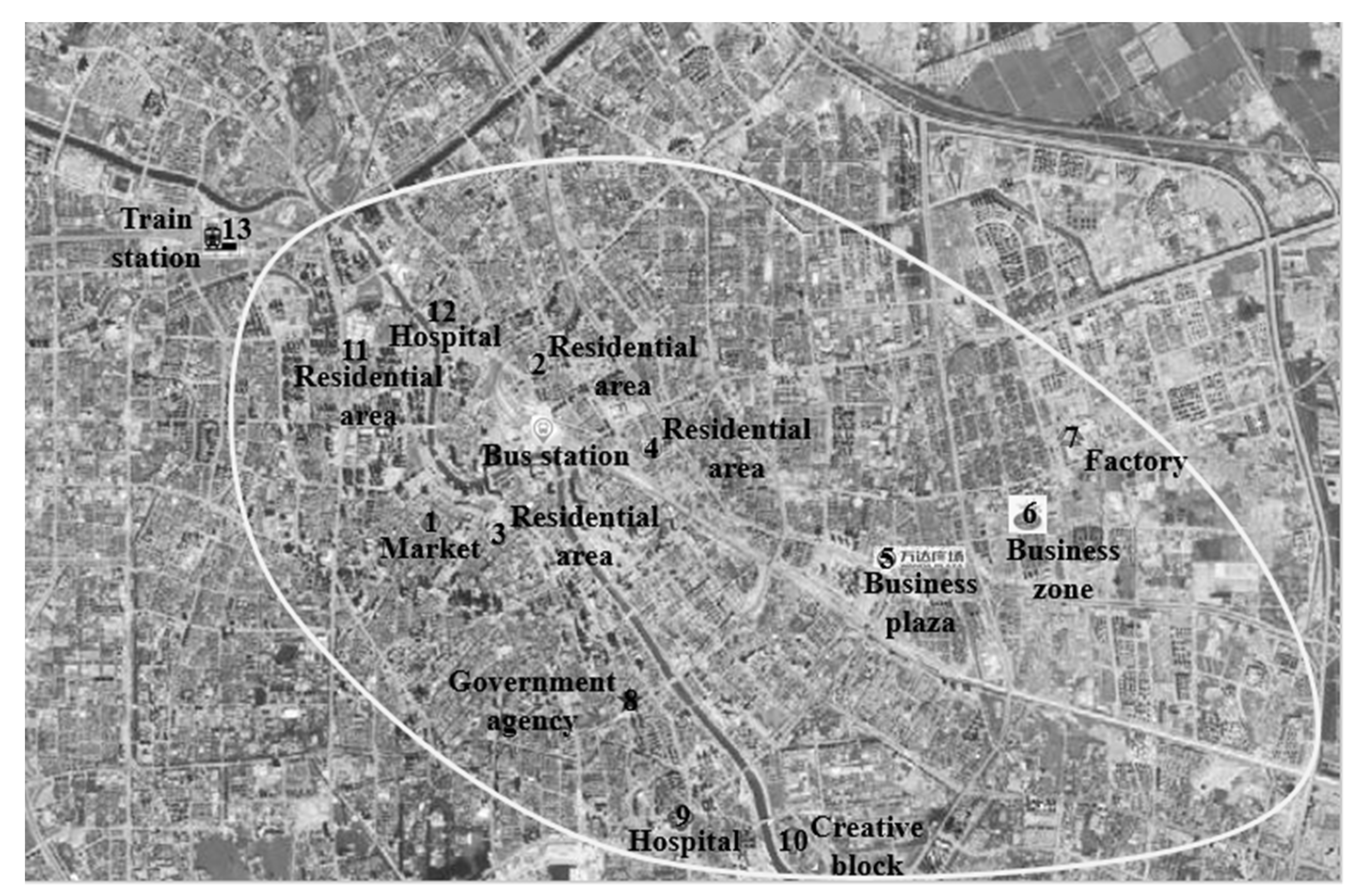
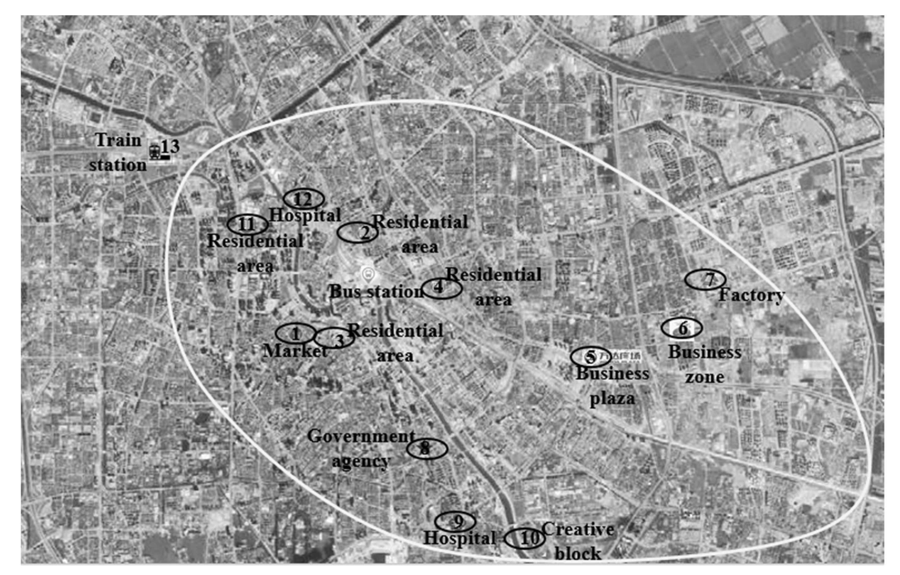
In this section, we analyze travel demands for the customized shuttle bus in an area served by a depot. We optimize the customized shuttle bus route in the decision period. The area is presented in Figure 2 and Figure 3. The K-means clustering analysis is adopted to analyze the travel demand and the result is shown in Figure 4. Passengers get on customized shuttle bus vehicles mainly in residential areas, while their destinations are mainly government agencies, hospitals, the central business district, enterprises, and creative industry parks. The number of pairs of origin-destination is 200 and this paper has not listed them all due to the limited space. There is a line between any two stops. The distances matrices are given in Table 1 and Table 2. The travel time depends on the traffic condition. The arrival time and dwell time are given by Table 3. and are normally distributed, while the expectation is 3 and the variance is 1. Under 90% confidence, all stops can be served in their time windows, which means that the chance constraint is as follows:
The capacity of a vehicle is 45 passengers. The fixed cost of a trip is USD 200 and unit operation cost is USD 2. The ticket fare is USD 10.
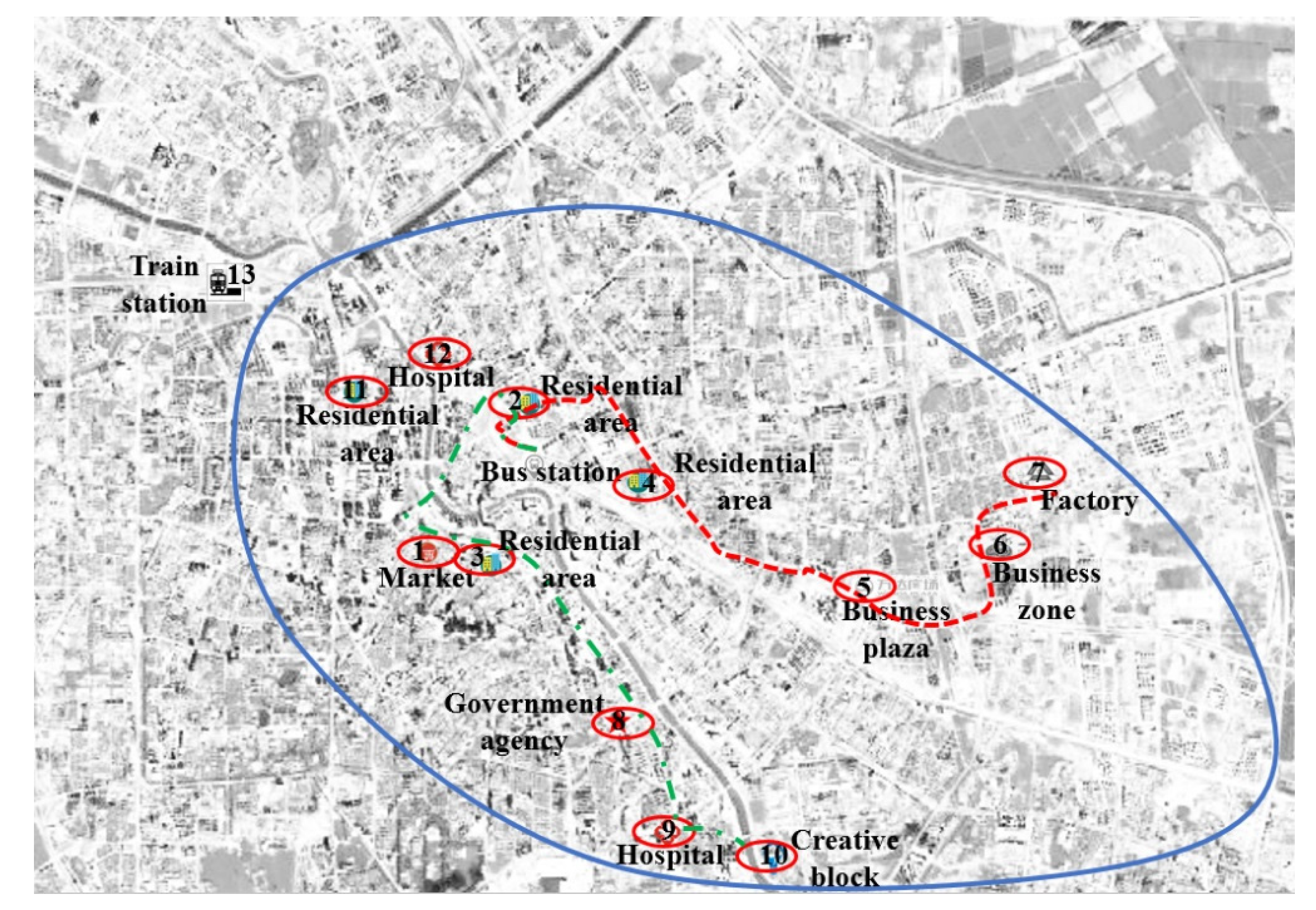
We adopt the following parameter values: The number of iterations is 1000, the number of clone operator times is 500, and the population size is 1200. The time for the calculation is 1.5 s. The optimized customized shuttle bus lines are shown in Figure 4. Two customized shuttle bus lines are obtained (2-4-5-6-7, 2-1-3-8-9-10) and 90% demands can be satisfied. To verify the practical effect of the model and algorithm, we compare the results for different travel demands, as shown in Table 4 and Table 5.
In the case of the same random time, compared with the traditional simulated annealing algorithm (the cooling rate is 0.98, the initial temperature is 1000, the end temperature is 0.001, and the chain length L of the Metropolis is 500), the proposed hybrid intelligent optimization algorithm can improve the solving efficiency of the model, especially when there is a large travel demand. The advantage of the proposed hybrid intelligent optimization algorithm is obvious in terms of the solving speed. The proportion of passengers served will be improved with the increasing of the travel demand. The simulated annealing algorithm works as follows:
| Step 1 |
| Initialization. Set a large enough initial temperature T0, T = T0, and determine the number of iterations of each T (that is, the chain length L of the Metropolis) by the randomly generated initial solution S. |
| Step 2 |
| For the current temperature T and k = 1, 2, ..., L, repeat Step 3 ~ 6. |
| Step 3 |
| A new solution S’ is generated by randomly perturbing the current solution S. |
| Step 4 |
| The increment d of S’ is calculated as f(S’) – f(S), where f(S) is the cost function of S. |
| Step 5 |
| If d < 0, then accept S’ as the new current solution; otherwise, calculate the acceptance exp(−d/T) of S’, and determine whether to retain S’ by comparing the value of the random number rand generated in (0,1) interval with the acceptance; if exp(−d/T) > rand, then accept S’ as the current solution, otherwise, retain S. |
| Step 6 |
| The termination condition of the algorithm is usually set as: In several continuous metropolis chains, the new solution S’ cannot be accepted, or reaches the set end temperature. If the termination condition of the algorithm is satisfied, the current solution will be the output as the optimal solution. Otherwise, the attenuation function T = qT (q is the cooling rate) attenuates T and returns to Step 2. |
5. Concluding Remarks
This work classifies passengers’ travel demand for a customized shuttle bus with the K-means clustering analysis. A customized shuttle bus line optimization model is established considering the operation cost and travel time requirement of passengers. Considering the delay of buses caused by the traffic jam, etc., a stochastic travel time constraint is included in the model. On the basis of the immune clonal algorithm, according to the characteristics of the model, the hybrid intelligent optimization algorithm is used to solve the model. Aiming at the chance constraint, a neural network is trained by the stochastic simulation technique to approximate the uncertain function. On this basis, the improved immune clonal algorithm is used to solve the problem. The effect of the model and algorithm is verified by the numerical example with different travel demand sizes. On the basis of the minimum cost, it can maximize the demand of the customized shuttle bus (90%), and ensure the travel time demand of passengers. This method can improve the efficiency of the customized shuttle bus line planning effectively, which is nearly 10 times faster than the traditional simulated annealing algorithm. By optimizing the customized bus routes, it can continuously improve the service quality and efficiency, promote the diversification of urban public transit, and improve the sharing of urban public transit. However, how to schedule vehicles after they arrive at the terminals is neglected and could be a path for future work.
Author Contributions
Conceptualization, K.Z.; data curation, X.Y. and R.S.; formal analysis, Z.S. and X.Y.; methodology, K.Z.; project administration, Z.S.; resources, X.P.; software, K.Z. and Z.S.; supervision, X.P.; validation, X.P. and Z.S.; writing—original draft, K.Z.; writing—review & editing, R.S. and X.Y. All authors have read and agreed to the published version of the manuscript.
Funding
The National Key Research and Development Program of China: 2018YFB1600900.
Acknowledgments
This paper is supported by the National Key Research and Development Program of China (no. 2018YFB1600900).
Conflicts of Interest
The authors declare no conflict of interest.
References
- Cao, Y.; Wang, J. The key contributing factors of customized shuttle bus in rush hour: A case study in Harbin City. Procedia Eng. 2016, 137, 478–486. [Google Scholar] [CrossRef] [Green Version]
- Lei, Y.W.; Lin, P.Q.; Yao, K.B. The network scheduling model and its solution algorithm of Internet customized shuttle bus. J. Transp. Syst. Eng. Inf. Technol. 2017, 17, 157–163. [Google Scholar]
- Cheng, L.Q. Study on the line network layout of customized shuttle bus planning of the level analysis method of point, line and plane. J. Dali. Jiaotong Univ. 2014, 35, 23–26. [Google Scholar]
- Pan, S.L.; Yu, J.; Yang, X.F.; Liu, Y.; Zou, N. Designing a flexible feeder transit system serving irregularly shaped and gated communities: Determining service area and feeder route planning. J. Urban Plan. Dev. 2014. [Google Scholar] [CrossRef]
- Pan, S.L.; Lu, X.L.; Zou, N. Route planning and coordinated scheduling model for flexible feeder transit service. J. Jilin Univ. (Eng. Technol. Ed.) 2016, 46, 1827–1835. [Google Scholar]
- Lin, B.L.; Yang, F.S.; Li, P. Designing optimal bus network for minimizing trip times of passenger flows. China J. Highw. Transp. 1999, 12, 79–83. [Google Scholar]
- Zhou, G.W.; Luo, X. Network layout optimization model of multi-modal comprehensive public transit system and simulation. Appl. Res. Comput. 2013, 30, 1035–1040. [Google Scholar]
- He, S.X.; Fan, B.Q. Optimal path searching algorithm in transit network. J. Transp. Eng. Inf. 2007, 5, 22–27. [Google Scholar]
- Mireia, R.R.; Miquel, E.; César, T. The design of interurban bus networks in city centers. Transp. Res. Part A 2012, 46, 1153–1165. [Google Scholar]
- Perugia, A.; Moccia, L.; Cordeau, J.F.; Laporte, G. Designing a home-to-work bus service in a metropolitan area. Transp. Res. Part B 2011, 45, 1710–1726. [Google Scholar] [CrossRef]
- Amiripour, S.M.M.; Ceder, A.; Mohaymany, A.S. Designing large-scale bus network with seasonal variations of demand. Transp. Res. Part C 2014, 48, 322–338. [Google Scholar] [CrossRef]
- Leksakul, K.; Smutkupt, U.; Jintawiwat, R.; Phongmoob, S. Heuristic approach for solving employee bus routes in a large-scale industrial factory. Adv. Eng. Inform. 2017, 32, 176–187. [Google Scholar] [CrossRef]
- Ouyang, A.F.; Nourbakhsh, M.S.; Cassidy, J.M. Continuum approximation approach to bus network design under spatially heterogeneous demand. Transp. Res. Part B 2014, 68, 333–344. [Google Scholar] [CrossRef]
- Chang, Y.L.; Hu, Q.Z. Optimal line model on urban public traffic line network. China J. Highw. Transp. 2005, 18, 95–98. [Google Scholar]
- Tom, V.M.; Mohan, S. Transit route network design using frequency coded genetic algorithm. J. Transp. Eng. 2003, 129, 186–195. [Google Scholar] [CrossRef]
- Wei, F.; Machemehl, B.R. Using a simulated annealing algorithm to solve the transit route network design problem. J. Transp. Eng. 2006, 132, 122–132. [Google Scholar]
- Wei, F.; Machemehl, R.B. Bi-level optimization model for public transportation network redesign problem. Transp. Res. Rec. J. Transp. Res. Board 2012, 2263, 151–162. [Google Scholar]
- Xu, G.M.; Shi, F.; Luo, X.; Qin, J. Method of public transit network planning based on strategy equilibrium transit assignment. J. Transp. Syst. Eng. Inf. Technol. 2015, 15, 140–145. [Google Scholar]
- Yu, L.J.; Liang, M.P. Urban routine bus transit network optimizing design based on integer nonlinear programming model. China J. Highw. Transp. 2016, 29, 108–115. [Google Scholar]
- Hu, Q.Z.; Deng, W.; Tian, X.X. Optimization model of public traffic network and ant algorithm with four dimensions consumption. J. Southeast Univ. (Nat. Sci. Ed.) 2008, 38, 304–308. [Google Scholar]
- Yu, B.; Yang, Z.Z.; Jin, P.H.; Wu, S.H.; Yao, B.Z. Transit route network design-maximizing direct and transfer demand density. Transp. Res. Part C 2012, 22, 58–75. [Google Scholar] [CrossRef]
- Zhao, F.; Zeng, X.G. Optimization of user and operator cost for large-scale transit network. J. Transp. Eng. 2007, 133, 240–251. [Google Scholar] [CrossRef]
- Szeto, Y.W.; Jiang, Y. Transit route and frequency design: Bi-level modeling and hybrid artificial bee colony algorithm approach. Transp. Res. Part B 2014, 67, 235–263. [Google Scholar] [CrossRef] [Green Version]
- Wang, Q.; Wang, C.; Feng, Z.Y.; Ye, J.F. Review of K-means clustering algorithm. Electron. Des. Eng. 2012, 20, 21–24. [Google Scholar]
- Liu, B.D.; Zhao, R.Q.; Wang, G. Uncertain Programming with Applications, 3rd ed.; Tsinghua University Press: Beijing, China, 2003; pp. 54–96. [Google Scholar]
- Li, L.; Li, H.Q.; Xie, S.L.; Li, X.Y. Immune particle swarm optimization algorithms based on clone selection. Comput. Sci. 2008, 35, 253–278. [Google Scholar]
Figure 1.
Schematic plot of antibody coding.

Figure 2.
Layout of the customized shuttle bus service demand points.

Figure 3.
Results of the cluster analysis.

Figure 4.
Schematic diagram of the customized shuttle bus routes planning.


Table 1.
Distance between the bus station and each stop (km).
| Stop | v1 | v2 | v3 | v4 | v5 | v6 | v7 | v8 | v9 | v10 | v11 | v12 |
|---|---|---|---|---|---|---|---|---|---|---|---|---|
| Distance | 4 | 1 | 1.5 | 6.5 | 11.5 | 14.5 | 17.5 | 5.5 | 8.5 | 10.5 | 5 | 4 |
Table 2.
Distance matrix among stops (km).
| v1 | v2 | v3 | v4 | v5 | v6 | v7 | v8 | v9 | v10 | v11 | v12 | |
|---|---|---|---|---|---|---|---|---|---|---|---|---|
| v1 | 0 | 4 | 1 | 6 | 11 | 15 | 18 | 5 | 8 | 10 | 4 | 6 |
| v2 | 4 | 0 | 5 | 2 | 7 | 10 | 13 | 9 | 12 | 14 | 4 | 3 |
| v3 | 1 | 5 | 0 | 7 | 12 | 15 | 18 | 4 | 7 | 9 | 5 | 7 |
| v4 | 6 | 2 | 7 | 0 | 5 | 8 | 11 | 11 | 14 | 16 | 6 | 5 |
| v5 | 11 | 7 | 12 | 5 | 0 | 3 | 6 | 16 | 19 | 21 | 11 | 10 |
| v6 | 15 | 10 | 15 | 8 | 3 | 0 | 3 | 19 | 22 | 24 | 14 | 13 |
| v7 | 18 | 13 | 18 | 11 | 6 | 3 | 0 | 22 | 25 | 27 | 17 | 16 |
| v8 | 5 | 9 | 4 | 11 | 16 | 19 | 22 | 0 | 3 | 5 | 9 | 11 |
| v9 | 8 | 12 | 7 | 14 | 19 | 22 | 25 | 3 | 0 | 2 | 12 | 14 |
| v10 | 10 | 14 | 9 | 16 | 21 | 24 | 27 | 5 | 2 | 0 | 14 | 16 |
| v11 | 4 | 4 | 5 | 6 | 11 | 14 | 17 | 9 | 12 | 14 | 0 | 3 |
| v12 | 6 | 6 | 7 | 5 | 10 | 13 | 16 | 11 | 14 | 16 | 3 | 0 |
Table 3.
Arrival time and waiting time of vehicles required by each stop.
| Stop | Arrival Time | Waiting Time (min) | Stop | Arrival Time | Waiting Time (min) |
|---|---|---|---|---|---|
| v1 | 8:00 | 2 | v7 | 8:50 | 2 |
| v2 | 8:10 | 2 | v8 | 8:20 | 2 |
| v3 | 8:05 | 2 | v9 | 8:30 | 2 |
| v4 | 8:15 | 3 | v10 | 8:35 | 1 |
| v5 | 8:30 | 2 | v11 | 8:05 | 2 |
| v6 | 8:40 | 2 | v12 | 8:10 | 2 |
Table 4.
Comparison of operation parameters of different travel demand.
| Travel Demand/Trip | Operation Time/s | Number of Vehicles | Service Rate/% |
|---|---|---|---|
| 200 | 1.5 | 4 | 85 |
| 500 | 1.7 | 10 | 88 |
| 1000 | 2.2 | 22 | 90 |
Table 5.
Comparison of operation time comparison (s).
| Solution Method | Travel Demand/Trip | ||
|---|---|---|---|
| 200 | 500 | 1000 | |
| Hybrid intelligent optimization algorithm | 1.5 | 1.7 | 2.2 |
| Simulated annealing algorithm | 5 | 11 | 21 |
Publisher’s Note: MDPI stays neutral with regard to jurisdictional claims in published maps and institutional affiliations. |
© 2021 by the authors. Licensee MDPI, Basel, Switzerland. This article is an open access article distributed under the terms and conditions of the Creative Commons Attribution (CC BY) license (http://creativecommons.org/licenses/by/4.0/).
Share and Cite
MDPI and ACS Style
Sun, Z.; Zhou, K.; Yang, X.; Peng, X.; Song, R. Optimization Method of Customized Shuttle Bus Lines under Random Condition. Algorithms 2021, 14, 52. https://0-doi-org.brum.beds.ac.uk/10.3390/a14020052
AMA Style
Sun Z, Zhou K, Yang X, Peng X, Song R. Optimization Method of Customized Shuttle Bus Lines under Random Condition. Algorithms. 2021; 14(2):52. https://0-doi-org.brum.beds.ac.uk/10.3390/a14020052
Chicago/Turabian StyleSun, Zhichao, Kang Zhou, Xinzheng Yang, Xiao Peng, and Rui Song. 2021. "Optimization Method of Customized Shuttle Bus Lines under Random Condition" Algorithms 14, no. 2: 52. https://0-doi-org.brum.beds.ac.uk/10.3390/a14020052
Note that from the first issue of 2016, this journal uses article numbers instead of page numbers. See further details here.